The variability of volatile organic compounds during a persistent fog-haze episode

A persistent fog-haze process associated with high pollution occurred in the northern suburbs of Nanjing from November to December 2013. Based on the comprehensive chemical and microphysical observations during the intense observation period, the composition characteristics, and variation rules of volatile organic compounds (VOCs) in the atmosphere under four weather conditions (slight haze, haze, fog, and dense fog) were compared and analyzed, the influencing factors for VOCs during extremely dense fog were discussed in more detail. The average concentrations of VOCs displayed as alkanes > aromatics > alkenes > alkynes, and their concentrations were ranked as dense fog > fog > haze > slight haze, the main factor contributing to the difference in concentrations of VOCs under different weather conditions is the boundary layer characteristics and photochemical reaction rate. Microphysical parameters such as liquid water content (LWC) were negatively correlated with VOCs concentration in dense fog (LWC>0.008 g m⁻³). Also, the concentration of VOCs showed an oscillating decrease in extremely dense fog (LWC>0.12 g m⁻³), and the total VOCs removal rate was close to 30%, which may be attributed to an indirect/direct removal effect, in which the enhanced collision and deposition of fog droplets promote the redistribution of VOCs gas-aqueous/particle partitioning, and remove them from the atmosphere by fog water.

1 Introduction

Volatile organic compounds (VOCs) are important precursors of atmospheric photochemical smog and secondary organic aerosols. Atmospheric VOCs are mainly oxidized by OH radicals, O₃, and NO₃ radicals, with the reaction with OH radicals accounting for the major part. VOCs can undergo a variety of photochemical reactions in the presence of shortwave radiation, with O₃ being one of the main reaction products, and some oxygenated VOCs can also be generated from some primary VOCs(Yuan et al., 2013). Secondary aerosols generated by VOCs through the oxidation process are important components of fine particulate matter and have a significant impact on the formation of haze (Izhar et al., 2019). Oxidation of VOCs also provides a range of water-soluble compounds (e.g., formaldehyde, glyoxal) that are partitioned into wet aerosols or cloud droplets at high relative humidity and further oxidized to produce new secondary organic compounds (Ervens et al., 2011). Secondary organic aerosol (SOA) can act as a condensation nucleus and thus affect the life history, size, and retention time of cloud droplets, and can be removed by nucleation and collision in the atmosphere (Herckes et al., 2013).

With economic development, severe O₃ and SOA pollution has become a widely recognized environmental issue, and these pollutants are particularly prominent in highly urbanized and industrial areas (Deng et al., 2019). The studying of VOCs is getting more and more attention because they are important precursors of O₃ and SOA and have important effects on human health. In China, most of the research on VOCs is focused on some high-pollution areas, such as the North China Plain, Yangtze River Delta, Pearl River Delta, and Central China (Dai et al., 2017; Sheng et al., 2018; Hui et al., 2019), and mainly focuses on the emission characteristics of VOCs, analysis of emission sources, and sensitivity to O₃ formation (Mozaffar and Zhang, 2020).

The presence of fog droplets has an important influence on the concentration distribution, reaction mechanisms, and removal processes of pollutants in the atmosphere (Collett et al., 2008). As fog often occurs in the stable inversion layer, fog droplets in the atmosphere are suspended for a long time and have a large surface area, so the concentration of pollutants in fog droplets can reach several times to dozens of times the rain droplets (Błaś et al., 2008). Fog droplets can also influence the processes of production and chemical reactions of several particulate matters, as well as their chemical composition, mass, and number concentration distribution, thus directly or indirectly affecting regional climate (Izhar et al., 2020). Aqueous phase processes are an important way to influence chemical processes in the atmosphere (Duan et al., 2021; Franco et al., 2021). In the aqueous phase, organic compounds are often oxidized by OH radicals (Ervens et al., 2014). In the presence of fog, some soluble organic compounds can be dissolved in the droplets and further oxidized in the droplets, resulting in chemical reactions different from those in the gas phase. After evaporation, the droplets can form hygroscopic secondary aerosol particles, which can further form haze when their concentration is high, realizing the fog-haze transformation (Pandis et al., 1990).

Due to the high solubility of oxygenated volatile organic compounds (OVOCs), fog has been found to have a significant wet scavenging effect on them (Sahu et al., 2016; Yang et al., 2017; Hakkim et al., 2019), while fewer studies have been conducted on the correlation between hydrophobic VOCs species and fog. It has been found that the concentration of insoluble VOCs in rainwater is higher than the value determined by Henry’s law, and precipitation may be an important mechanism for the removal of VOCs(Okochi et al., 2004; Sato et al., 2006; Šoštarić et al., 2017); However, it has also been suggested that for hydrophobic VOCs like benzene, wet deposition is not an effective mechanism for the removal of these pollutants from the atmosphere (Mullaugh et al., 2015), solubility did not significantly affect the concentration of VOCs in foggy days (Hakkim et al., 2019). In general, the exact mechanism of VOCs in the gas-aqueous phase process is still unclear, there are still fewer studies on the fog-haze transformation process, especially the effect of extremely dense fog on VOCs(Gilardoni et al., 2014; Hakkim et al., 2019). This study will use the combined physicochemical observations of VOCs and fog during a persistent high pollution process in Nanjing from 30 November to 12 December 2013 (UTC+8, same below) to analyze the composition characteristics and variation of atmospheric VOCs under four weather conditions (slight haze, haze, fog, and dense fog), and focus on the influencing factors of VOCs concentration changes under dense fog conditions.

2 Materials and methods

2.1 Observation sites and instruments

The VOCs and pollutant gases observation instruments were located in the campus of Nanjing University of Information Science and Technology, Pukou District, Nanjing (118°42′E, 32°20′N, altitude: 62 m). The observations of fog droplet spectra and meteorological elements are located in the integrated observation training practice base of China Meteorological Administration on campus. The northeast direction of the observation site includes the petrochemical industry, iron, and steel plants and chemical plants, and other large enterprises in the north industrial area of Nanjing. 500 m east of the VOCs observation site is the north-south Ningliu Highway, and the information from the observation site in this area can represent a composite source of traffic, urban, industrial and arable land, as seen in Figure 1. Details of the instruments are shown in Table 1.

FIGURE 1

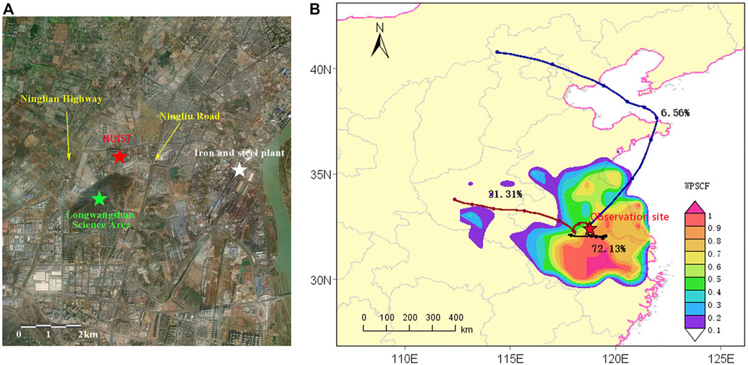
FIGURE 1. (A). Surrounding of the observation site (B). The 72 h air mass back trajectories and potential source contribution function (PSCF) analysis of VOCs.

TABLE 1

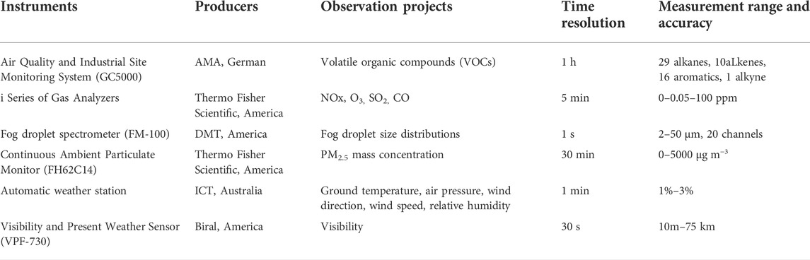
TABLE 1. Observation instruments.

2.2 Calculation method

2.2.1 Droplet spectrum data processing of fog

Droplet concentration N (in units of cm⁻³) and liquid water content LWC (in units of g·m⁻³) are calculated using the expression:

$\begin{array}{c}\mathit{N}={\displaystyle \sum }_{\mathit{i}=\mathbf{2}}^{\mathbf{20}}\mathit{n}\left({\mathit{r}}_{\mathit{i}}\right)∆\mathit{r}\end{array}(1)$

$\begin{array}{c}\mathit{L}\mathit{W}\mathit{C}=\mathbf{1}\times {\mathbf{10}}^{-\mathbf{6}}\times \mathit{\rho }\times {\displaystyle \sum }_{\mathit{i}=\mathbf{2}}^{\mathbf{20}}\frac{\mathbf{4}\mathit{\pi }}{\mathbf{3}}{\mathit{r}}_{\mathit{i}}^{\mathbf{3}}\mathit{n}\left({\mathit{r}}_{\mathit{i}}\right)∆\mathit{r}\end{array}(2)$

where $r_i$ (in units of μm) is the droplet radius, $n\left(r_i\right)$ (in units of cm⁻³·μm⁻¹) is the droplet size distribution. ρ = 1g·cm⁻³ is the density of water.

T_f is the threshold function describing the threshold behavior of the autoconversion process. The size truncation function employed to quantify the effect of truncating the cloud droplet size distribution on the autoconversion rate can be used as a threshold function to represent the threshold behavior associated with the autoconversion process, providing a physical basis for the threshold function. The value of T_f is between 0 and 1, and the larger the value, the stronger the process of collision, T_f = 0 means no collision process, T_f = 1 means complete collision process. It can be generally described by:

$\begin{array}{c}{\mathit{T}}_{\mathit{f}}=\frac{\mathit{P}}{{\mathit{P}}_{\mathbf{0}}}=\left[\frac{{\int }_{{\mathit{r}}_{\mathit{c}}}^{\mathbf{\infty }}{\mathit{r}}^{\mathbf{6}}\mathit{n}\left(\mathit{r}\right)\mathit{d}\mathit{r}}{{\int }_{\mathbf{0}}^{\mathbf{\infty }}{\mathit{r}}^{\mathbf{6}}\mathit{n}\left(\mathit{r}\right)\mathit{d}\mathit{r}}\right]\left[\frac{{\int }_{{\mathit{r}}_{\mathit{c}}}^{\mathbf{\infty }}{\mathit{r}}^{\mathbf{3}}\mathit{n}\left(\mathit{r}\right)\mathit{d}\mathit{r}}{{\int }_{\mathbf{0}}^{\mathbf{\infty }}{\mathit{r}}^{\mathbf{3}}\mathit{n}\left(\mathit{r}\right)\mathit{d}\mathit{r}}\right]\end{array}(3)$

$\begin{array}{c}{\mathit{r}}_{\mathit{c}}\approx \mathbf{4.09}\times {\mathbf{10}}^{-\mathbf{4}}{\mathit{\beta }}_{\mathit{c}\mathit{o}\mathit{n}}^{\frac{\mathbf{1}}{\mathbf{6}}}{\mathit{N}}^{\frac{\mathbf{1}}{\mathbf{6}}}{\mathit{L}\mathit{W}\mathit{C}}^{-\frac{\mathbf{1}}{\mathbf{3}}}\end{array}(4)$

where P is the autoconversion rate, P₀ is the rate function describing the conversion rate after the onset of the autoconversion process, ${\beta }_{con}=1.15\times {10}^{23}$ is an empirical coefficient, r_c is the critical radius for autoconversion (Liu, 2005; Niu et al., 2010).

V_t is the LWC weighted particle terminal velocity (in units of cm·s⁻¹) which can be described by:

$\begin{array}{c}{\mathit{V}}_{\mathit{t}}=\frac{\left(\frac{\mathbf{4}}{\mathbf{3}}\right)\mathit{\pi }\mathit{\rho }{\displaystyle \sum }_{\mathit{i}=\mathbf{2}}^{\mathbf{20}}{\mathit{n}}_{\mathit{i}}{\mathit{r}}_{\mathit{i}}^{\mathbf{3}}{\mathit{v}}_{\mathit{i}}}{\mathit{L}\mathit{W}\mathit{C}}\end{array}(5)$

$\begin{array}{c}{\mathit{v}}_{\mathit{i}}=\mathbf{1.202}\times {\mathbf{10}}^{-\mathbf{2}}{\mathit{r}}_{\mathit{i}}^{\mathbf{2}}\end{array}(6)$

where v_i (in units of cm·s⁻¹) is the fog droplets terminal velocities for each size interval (Gultepe and Milbrandt, 2007).

2.2.2 Trajectory data

The backward trajectory is calculated by the Hybrid Single-Particle Lagrangian Integrated Trajectory (HYSPLIT) model developed by NOAA. It is widely used to analyze the sources and transport pathways of pollutants. Cluster analysis is the analytical process of grouping a collection of data objects into multiple classes composed of similar objects, and is a multivariate analytical tool for studying multivariate classification. In this paper, the Trajstat plug-in in Meteoinfo software is used to perform cluster analysis on the backward trajectory. 72 h backward trajectories of air masses from 0:00 to 23:00 are calculated, with an altitude of 500 m. Meteorological data are from the Global Data Assimilation System (http://www.arl.noaa.gov/).

The potential source contribution function (PSCF) is used for further analysis of the sources of pollutants (Draxler and Hess, 1998). The PSCF value for a given grid cell is calculated by counting the trajectory segment endpoints that are terminate within the grid cell, and is defined as:

$\begin{array}{c}{\mathit{P}\mathit{S}\mathit{C}\mathit{F}}_{\mathit{i}\mathit{j}}=\frac{{\mathit{m}}_{\mathit{i}\mathit{j}}}{{\mathit{n}}_{\mathit{i}\mathit{j}}}\end{array}(7)$

where $m_{ij}$ is the number of endpoints, $n_{ij}$ is the total number of endpoints that fall in the cell. To minimize the error, an empirical weight function $W_{ij}$ is applied: ${WPSCF}_{ij}=W_{ij}\times {PSCF}_{ij}$, and $W_{ij}$ is defined as:

$\begin{array}{c}{\mathit{W}}_{\mathit{i}\mathit{j}}=\{\begin{array}{c}\mathbf{1.00}\mathbf{4}{\mathit{n}}_{\mathit{a}\mathit{v}\mathit{e}}<{\mathit{n}}_{\mathit{i}\mathit{j}}\\ \mathbf{0.70}{\mathit{n}}_{\mathit{a}\mathit{v}\mathit{e}}<{\mathit{n}}_{\mathit{i}\mathit{j}}\le \mathbf{4}{\mathit{n}}_{\mathit{a}\mathit{v}\mathit{e}}\\ \mathbf{0.42}\mathbf{0.5}{\mathit{n}}_{\mathit{a}\mathit{v}\mathit{e}}<{\mathit{n}}_{\mathit{i}\mathit{j}}\le {\mathit{n}}_{\mathit{a}\mathit{v}\mathit{e}}\\ \mathbf{0.05}{\mathit{n}}_{\mathit{i}\mathit{j}}\le \mathbf{0.5}{\mathit{n}}_{\mathit{a}\mathit{v}\mathit{e}}\end{array}\end{array}(8)$

where n_ave is the average number of trajectory segment endpoints per grid.

2.2.3 Ventilation coefficient

Ventilation coefficient (VC) is a product of boundary layer height and average wind speed through the mixing layer, it is used to characterize the transport rate of pollutants in the boundary layer in the horizontal direction. VC is calculated by:

$\mathit{V}\mathit{C}=\mathit{W}\mathit{S}\times \mathit{P}\mathit{B}\mathit{L}\mathit{H}$

where WS (in units of m·s⁻¹) is average wind velocity near the ground, PBLH (in units of m) is boundary layer height. PBLH data are from the Global Data Assimilation System.

3 Result

3.1 Meteorological condition and microphysical parameters

The observation period was divided into four weather conditions (slight haze, haze, fog, and dense fog) based on visibility (VIS) and relative humidity (RH). The specific classification criteria are shown in Table 2(Deng et al., 2002; Niu et al., 2016; Jiang et al., 2017). Figure 2 shows the complete fog-haze interconversion process during a persistent high pollution event in Nanjing from 1 December 2013, to 12 December 2013. As shown in Figure 2A, there is a negative correlation between VIS and RH, fog and haze exist alternately. During the observation period, a total of five gradually intensifying fog processes occurred, which are labeled as F1, F2, F3, F4, and F5 for the convenience of description. It can be seen that: F1, F2, and F3 occurred in the early morning hours of December 4, 5, and 6, which is due to the easy formation of an inversion layer in the boundary layer in winter and the formation of radiation fog near the surface, this kind of fog gradually dissipates after sunrise due to the surface warming and the destruction of the stable layer. F4 lasted longer and was more intense, with visibility reduced to below 100 m, but lasted no more than 2 h, and the fog dissipated briefly in the afternoon due to enhanced shortwave radiation. It was followed by F5 in the afternoon of 7 December to the early morning of 9 December, the process was the most intense and longest lasting, during which visibility decreased to below 50 m and lasted close to 31 h.

TABLE 2

TABLE 2. The judgment criteria of slight haze, haze, fog, and dense fog.

FIGURE 2

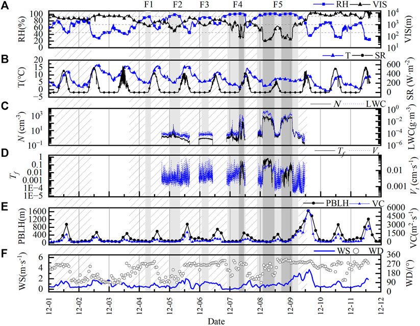
FIGURE 2. Temporal evolutions of the meteorological elements and fog microphysical variables in the period of observation. [(A). Visibility and relative humidity, (B). Short-wave radiation intensity and air temperature, (C). The number concentration of fog (black line) and liquid water content (blue line), (D). Autoconversion threshold function (T_f) and weighted particle terminal velocity (V_t), (E). Planetary boundary layer height (PBLH) and ventilation coefficient (VC), (F). Wind speed and wind direction. Slash area represents haze events, the light grey shade represents fog events, the dark grey shade represents dense fog events, and slight haze events are the rest.].

3.2 Composition and variation of VOCs

A total of 56 VOCs were measured during the observation period, which were classified into four categories according to their functional groups: alkanes, alkenes, alkynes, and aromatics. Figure 3 shows the average mixing ratio of VOCs under four weather conditions, and the specific mixing ratio of each species is shown in Supplementary Table S1. Compared with the observations in Nanjing during the same period (Li et al., 2013), the mixing ratio of VOCs under slight haze conditions were comparable to the annual average concentrations, while the mixing ratio of VOCs under other weather conditions were significantly higher.

FIGURE 3

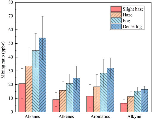
FIGURE 3. The average volume fraction of each component in atmospheric VOCs during different weather conditions.

Figure 4 shows the time-series variation of pollutants, where slash area represents haze events, the light grey shade represents fog events, the dark grey shade represents dense fog events, and light haze events are the rest. With constant fluctuations in VOCs concentrations from December 1st to fourth, especially for alkanes (Figure 4A), and a brief peak in total VOCs (TVOCs) concentration of 149.12 ppbv was observed on December 2nd at the end of first haze process. The TVOCs concentration increased on the fourth and the weather turned to haze again, with the highest TVOCs reaching 181.36 ppbv after the brief fog process F1 ended. F2 occurred in the early morning of the fifth, when TVOCs reached 84.06 ppbv, followed by a decrease in VOCs concentrations, which may be attributed to photochemical reaction and realatively high VC compared to previous days. F3 occurred in the morning of 6 December, during which small peaks appeared. F4 started from the evening of 6 December , along with the gradual increase in the intensity of the fog, VOCs concentration reached a peak of 133.56 ppbv during the dense fog, then the fog dissipated briefly at noon on the seventh, VOCs concentration fell back a little, and the weather turned to haze. The longest dense fog process F5 occurred on the eighth and lasted until the morning of the ninth, during which VOCs concentration increased again and reached a peak of 190.89 ppbv after two fluctuations. It is notable that when the dense fog changed to extremely dense fog during F5, the VOCs concentration showed a different degree of decrease, and we will focus on this issue in Section 3.5 to understand it quantitatively.

FIGURE 4

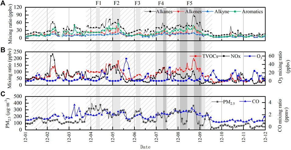
FIGURE 4. Temporal variations of pollutants during the period of intensive observation. [(A). Alkanes, Alkenes, Alkynes, and Aromatics. (B).TVOCs, NOx, and O₃. (C). PM_2.5 and CO. Light grey shade represents fog events, dark grey shade represents dense fog events, and slight haze events are the rest.].

3.3 Spatially sources of VOCs

In order to quantitatively analyze the VOCs pollution transport, the HYSPLIT model was used to analyze the 72 h backward trajectory clustering of air masses at the observation site. The results of trajectory clustering and PSCF analysis of VOCs are given in Figure 1B the observed site during the pollution period from 4 December to 8 December was mainly influenced by three directional air masses from the south, northwest, and northeast, accounting for 72.13%, 21.31%, and 6.56%, respectively. The distribution of potential contribution of VOCs concentration shows that the area of high PSCF values is located in the south and southeast of the observation site, and the high PSCF values (0.8–1.0) occurred within 300 km south of the observation site, which means that the probability of VOCs concentration exceeding the set threshold (median VOCs concentration) for the backward trajectory of all air masses passing through this area is more than 80%, demonstrating the high potential source contribution of southwestern Jiangsu Province and southeastern Anhui Province to the VOCs concentrations at the observation site. On the whole, the potential source contribution of the VOCs pollutants was mainly influenced by the short-range transport of the Yangtze River Delta.

Also, the ratio of toluene to benzene (T/B) was used to identify local sources of pollution. T/B < 2 indicates that the pollutants are significantly affected by traffic emissions, and the larger the value of T/B, the more influenced by other emission sources; T/B > 2 indicates that there are other sources besides traffic emissions; when T/B reaches 10 or even higher, it indicates that there are strong industrial emission sources nearby (Hui et al., 2018). The mean value of T/B during the observation period is 1.21, which is consistent with the results measured by others in the northern suburbs of Nanjing (An et al., 2014), indicating that the emissions during the observation period are in line with the local average and that the emissions from traffic sources are more influential.

3.4 Differences in VOCs concentration under different weather conditions

The average concentration of VOCs during the observation period behaved as dense fog > fog > haze > slight haze, and this difference indicates that weather conditions have an important influence on the VOCs concentration characteristics. Table 3 shows that PBLH and VC are significantly lower on foggy (fog and dense fog) days than on hazy (haze and slight haze) days. The average PBLH and VC during dense fog are only 146 m and 119.16 m²-s⁻¹, respectively, which are the lowest among the four polluted weather conditions. The atmospheric boundary layer under static weather conditions is not conducive to the diffusion of atmospheric pollutants, resulting in the accumulation of VOCs pollutant (Hakkim et al., 2019). Also, radiation plays an important role in the photochemical process (Herckes et al., 2013), VOCs can be oxidized by O₃, NO₃, and OH radicals, which is the most dominant photochemical reaction process with OH radicals, while the non-photochemical reaction process with O₃ and NO₃ is much less influential (Hui et al., 2018). As can be seen in Figure 2B, shortwave radiation (SR) peaks daily in the late afternoon, showing significant daily variation characteristics, and the surface SR during F5 (8 December) was significantly reduced due to the weakening effect of dense fog. On the seventh day, the SR value reached 425 W m^−2, while the highest SR value on the eighth day was only 269 W m⁻², which weakened by 37%. This resulted in a significant reduction in the rate of production of reactive radicals, slowing down the photochemical reaction rate of VOCs. It can also be seen in Figure 4B that O₃, the main product of photochemical reactions, was significantly reduced during the dense fog with lower SR, while TVOCs maintained high oscillations, which indicated that the absence of photochemical reaction was one of the essential factors leading to the accumulation of VOCs. It can be seen that the differences in VOCs concentrations under different weather conditions were mainly influenced by boundary layer characteristics (such as wind speed, boundary layer height, and ventilation coefficient), as well as photochemical reaction rates.

TABLE 3

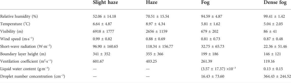
TABLE 3. Mean values ±standard deviation of meteorological elements and fog microphysical parameters in different weather conditions.

3.5 Effect of dense fog on the concentration of VOCs

Due to the accumulation of VOCs in boundary layer, the average concentration of TVOCs in dense fog is about 2.6 times higher than in slight haze. However, when F5 fog changed into extremely dense fog (VIS <50 m), the microphysical parameters of fog increased explosively, and the VOCs concentration showed a downward trend, the concentration of TVOCs even decreased from 204.56 ppbv to 125.3 ppbv by about 38% during the fog period from the eighth at 17:00 to the ninth at 0:00. The same phenomenon occurs with PM_2.5, which dropped from 362 μg m⁻³–77 μg m⁻³. Throughout the two periods of dense fog in F5, the average VC was 106.97 m² s⁻¹, and the degree of CO variation as a less reactive gas (Figure 4C) was also weak (1.26–3.24 ppbv), which shows that the atmospheric horizontal transport contributed little variation to the VOCs concentration. At the same time, the mean value of LWC during dense fog reached 0.13 g m⁻³, and the peak LWC reached 0.6 g m⁻³ during this observation, which is significantly higher than the observed values of fog in related studies (Yang et al., 2017; Hakkim et al., 2019), and such intensity and duration are also rare in the YRD area, which undoubtedly provides a rare opportunity to discuss the mechanism of the effect of dense fog on VOCs.

Although hydrophobic VOCs are poorly soluble, a higher droplet surface area may still affect the extent of VOCs dissolution in droplets at very high LWC in some degree (Herckes et al., 2013). To explore this possibility, we selected 10 VOCs species among 56 VOCs with significant solubility differences and a relatively large share of TVOCs concentration (total concentration share over 65% of TVOCs), compared and analyzed the differences in average VOCs concentration during dense fog (200 m ≥ VIS>50 m) extremely dense fog (VIS≤50 m). Table 4 ranks the VOCs components by solubility from largest to smallest according to Henry’s coefficient (Sander, 2015), and the mean concentration ratio ${\delta }_c$ is given (extremely dense fog/dense fog), which can be calculated by Eq. 10. To remove the effect of dilution, mean concentration ratio ${\delta }_c$ is revised by ventilation coefficient (Hakkim et al., 2019):

$\begin{array}{c}{\mathit{\delta }}_{\mathit{c}}=\frac{{\mathit{c}}_{\mathbf{2}}/{\mathit{V}\mathit{C}}_{\mathbf{2}}}{{\mathit{c}}_{\mathbf{1}}/{\mathit{V}\mathit{C}}_{\mathbf{1}}}\end{array}(10)$

where c₁ and c₂ are the concentration of VOCs and PM_2.5 under dense fog and extremely dense fog conditions; VC₁ and VC₂ are the average ventilation coefficients under dense fog and extremely dense fog conditions, respectively.

TABLE 4

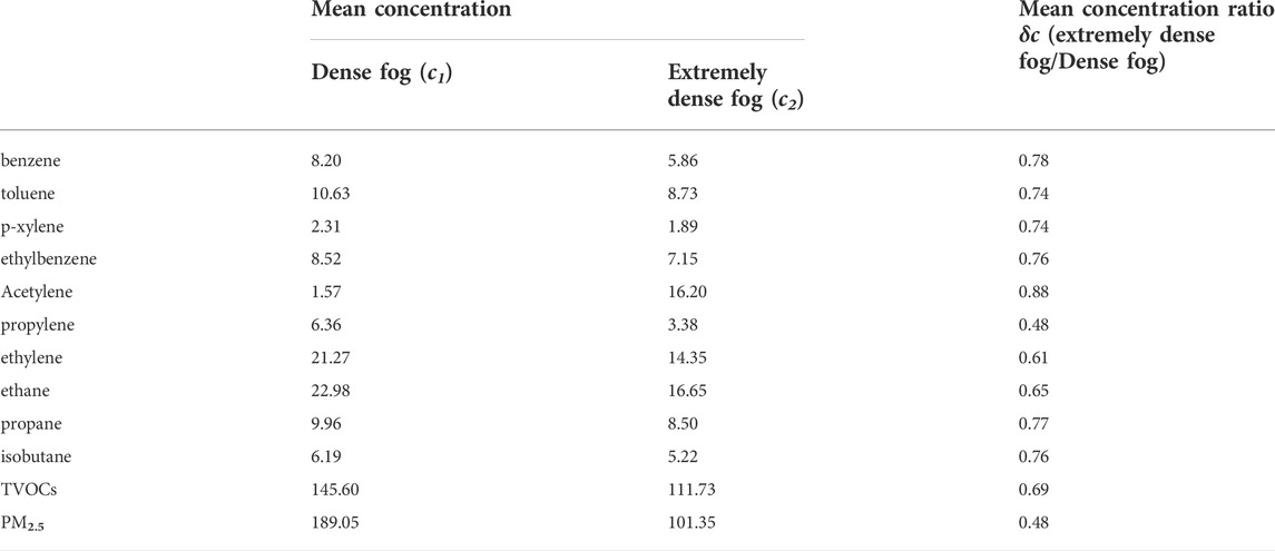
TABLE 4. Differences in concentrations of major VOCs (in units of ppbv) components and PM_2.5 (in units of μg·m⁻³) under dense fog and extremely dense fog events.

Table 4 shows that for each VOCs component, the variation of ${\delta }_c$ ranges from 0.48 to 0.88, with ${\delta }_c$ for TVOCs reaching 0.69 (removal rate close to 30%), indicating that the concentration of VOCs in extremely dense fog is significantly lower than in dense fog. Since the average ventilation coefficient was only 119.16 m² s⁻¹, it was obvious that the effect of horizontal transport was weak. According to Henry’s coefficient, the solubility ranking of VOCs is benzene > toluene > p-xylene > ethylbenzene > acetylene > propylene > ethylene > ethane > propane > isobutane. As can be seen in Table 4, there is no significant correlation between ${\delta }_c$ and the solubility of each component in dense fog and extremely dense fog, where acetylene has the weakest removal effect, while propylene has a slightly lower solubility than acetylene, but its removal effect is similar to PM_2.5 (more than 50%), which indicates that even in extremely dense fog with high LWC, the difference in the ambient VOCs concentration is not significantly influenced by the solubility. Therefore, the relationship between ambient VOCs concentrations and fog microphysical parameters needs to be further analyzed.

During the extremely dense fog, the fog body underwent explosive growth, and the average LWC value increased from 4.58 × 10⁻⁴ g m⁻³ to 0.23 g m⁻³ within half an hour at around 02:00 on the eighth, and all other microphysical parameters also increased significantly (Li et al., 1999), so the autoconversion threshold function T_f and the LWC weighted particle terminal velocity V_t was introduced to quantitatively explore the relationship between fog microphysics and VOCs concentration, their timing variations are shown in Figure 2D, Figure 5 shows the relationship between LWC and the concentrations of each component of VOCs, where the correlation between the two changes from positive to negative as LWC increases, and this turning point occurs at LWC ≈0.008 g m⁻³. For illustration purposes, a power-law relationship between VIS and LWC in fog was fitted with Eq. 11:

$\begin{array}{c}\mathit{V}\mathit{I}\mathit{S}=\mathbf{0.022}\times {\mathit{L}\mathit{W}\mathit{C}}^{-\mathbf{0.398}}\left({\mathbf{R}}^{\mathbf{2}}=\mathbf{0.87}\right)\end{array}(11)$

FIGURE 5

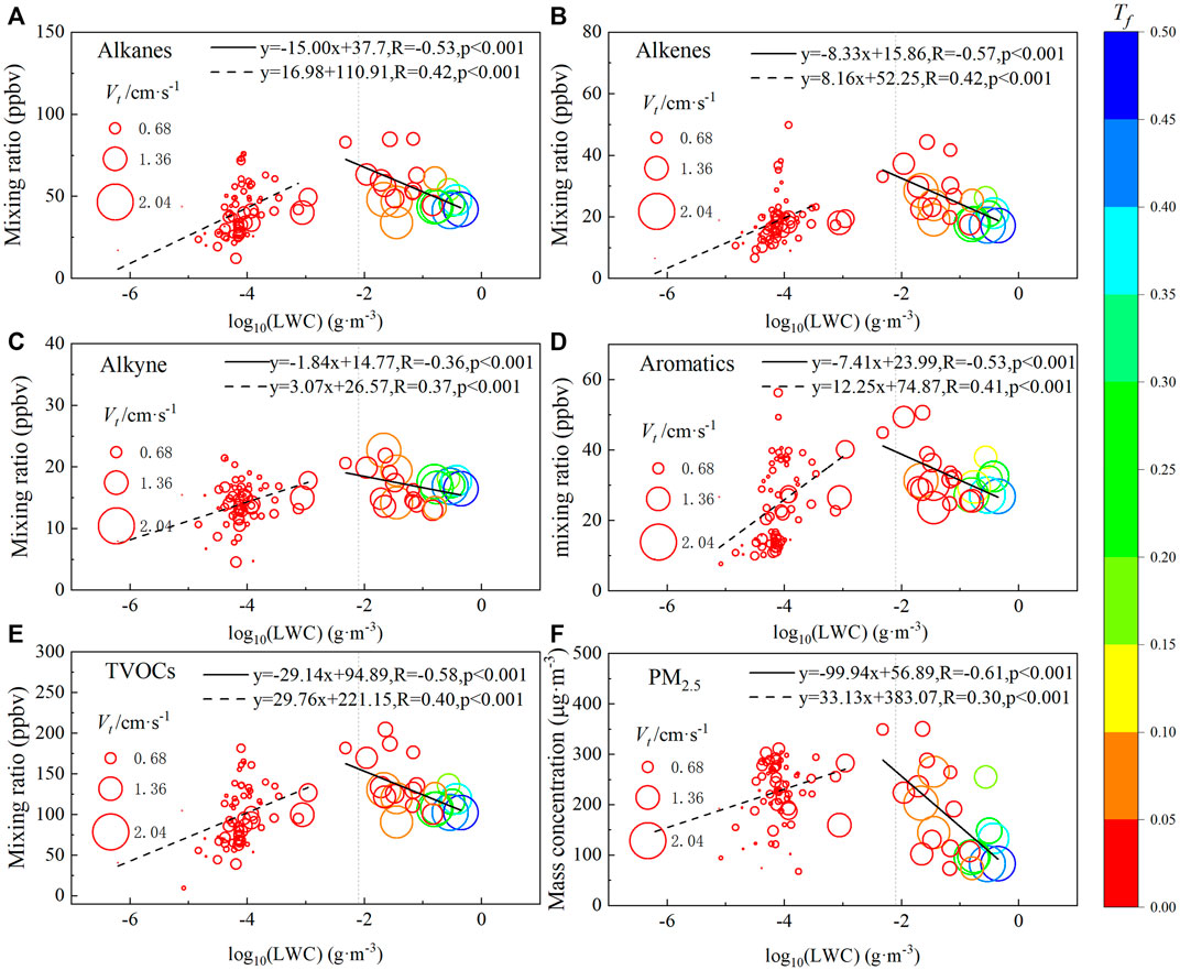
FIGURE 5. The relationship between microphysical variables of fog and (A). alkanes, (B). akenes, (C). alkynes, (D). aromatics, (E). TVOCs, (F). PM_2.5. [Horizontal axis is the logarithm of LWC with a base of 10, the vertical axis is the concentrations of VOCs, the sizes of bubbles represent mass-weighted particle terminal velocity, the colors of symbols represent the values of autoconversion threshold function].

As this process is influenced by the haze transformation, the contribution of hygroscopic aerosol extinction is not negligible, and at LWC = 0.008 g m⁻³, the corresponding VIS average is already close to 150 m, which is close to the average result given by the parameterization scheme for fog visibility in the North China Plain (about 220 m) (Zhang et al., 2014). Although the T_f value is still less than 0.05 at this time, V_t is already close to 1.36 cm s⁻¹, indicating that it is in the transitional stage of conversion from dense fog to extremely dense fog. When LWC>0.008 g m⁻³, as the fog body continuously enhances and VIS drops below 50 m (LWC>0.12 g m⁻³), the peak values of T_f and V_t reach 0.5 and 2.04 cm s⁻¹, respectively, and the large values of T_f and V_t are distributed in the lower right of the respective coordinates, i.e., the area of small (large) values of VOCs (LWC), which indicates that LWC, V_t and fog water deposition fluxes were significantly enhanced during the burst reinforcement of fog dominated by collision. In addition, it can be inferred from the slope of the fitted line between strong fog LWC versus VOCs and PM_2.5 in Figure 5: Extremely dense fog has the highest removal rate of PM_2.5, while the removal rates of alkanes, aromatics, and alkenes are closer among the components of VOCs, except alkynes, which was consistent with the inference given by ${\delta }_c$ in Table 4. This may be due to the fact that aerosol water formed by moisture absorption of fog droplets and aerosol can act as a tiny reactor for several reactions between gases and aerosols, resulting in complex gas-aqueous phase chemical reactions in the atmosphere (Ervens et al., 2011; Ervens, 2015), affecting the source-sink pathways of VOCs; VOCs may also be removed by adsorption and deposition at the gas-aqueous interface or on the surface of the particles (Raja and Valsaraj, 2004; Škrdlíková et al., 2011), and these processes are important factors influencing the variation of VOCs concentrations. The enhanced droplet collision effect may have promoted the redistribution of VOCs gas-aqueous/particle partitioning and removed VOCs from the atmosphere by an indirect/direct removal effect. Nevertheless, the specific physicochemical processes involved require more detailed measurements of the composition in fog water to better investigate the source-sink pathways of VOCs under the influence of fog in the future.

4 Conclusion

During the sustained high pollution period from November to December 2013, the average concentration of VOCs was alkanes > aromatics > alkenes > alkynes. as shown by the backward trajectory clustering and PSCF potential source contribution analysis: southwestern Jiangsu Province and southeastern Anhui Province have a high potential source contribution to the VOCs concentration at the observation site, indicating that the potential source contribution of the VOCs pollutants was mainly influenced by the short-range transport of the Yangtze River Delta.

The average concentration ranking of each VOCs component under four weather conditions was dense fog > fog > haze > slight haze. Compared with hazy days, the boundary layer height, ventilation coefficient, and short-wave radiation were significantly lower in foggy days, and the mean values of ventilation coefficient and short-wave radiation in dense fog were 119.16 m²·s⁻¹ and 22.36 W m⁻², which only accounted for about 20% of those in slight haze. It can be seen that the differences in VOCs concentrations under different weather conditions are mainly influenced by boundary layer characteristics as well as photochemical reaction rates.

There was no significant correlation between the mean concentration ratio ${\delta }_c$ of each VOCs components and its solubility in dense fog and extremely dense fog. The linear relationship between LWC versus VOCs and PM_2.5 was quantitatively analyzed on foggy days, and the threshold of occurrence of the correlation from positive to negative was at LWC ≈0.008 g m⁻³. In addition, extremely dense fog (LWC >0.12 g m⁻³) had a significant wet scavenging effect on PM_2.5 and VOCs, as deduced from the slope of the linear fit line: the highest scavenging rate for PM_2.5, followed by alkanes, aromatics and alkenes were closer to each other, and the lowest was for alkynes. To better investigate the source-sink pathways of VOCs under the influence of fog, the specific physicochemical processes involved require more detailed measurements of the composition in fog water in the future.

Data availability statement

The original contributions presented in the study are included in the article/Supplementary Material, further inquiries can be directed to the corresponding author.

Author contributions

YZ (First author): Methodology, drawing analysis, writing; JL: Methodology, writing, review and editing, supervision; YZ (Third author): Review and editing; JA: Observation; BZ: Review and editing.

Funding

This research was supported by the National Natural Science Foundation of China (Grant No. 41675136, 41875170, 42075177, 41675132, 42075186), Guangxi Key Research and Development Program (Grant No. AB20159013).

Conflict of interest

The authors declare that the research was conducted in the absence of any commercial or financial relationships that could be construed as a potential conflict of interest.

Publisher’s note

All claims expressed in this article are solely those of the authors and do not necessarily represent those of their affiliated organizations, or those of the publisher, the editors and the reviewers. Any product that may be evaluated in this article, or claim that may be made by its manufacturer, is not guaranteed or endorsed by the publisher.

Supplementary material

The Supplementary Material for this article can be found online at: https://www.frontiersin.org/articles/10.3389/fenvs.2022.1069905/full#supplementary-material

References

An, J., Zhu, B., Wang, H., Li, Y., Lin, X., and Yang, H. (2014). Characteristics and source apportionment of VOCs measured in an industrial area of Nanjing, Yangtze River Delta, China. Atmos. Environ. 97, 206–214. doi:10.1016/j.atmosenv.2014.08.021

CrossRef Full Text | Google Scholar

Błaś, M., Sobik, M., and Twarowski, R. (2008). Changes of cloud water chemical composition in the Western Sudety Mountains, Poland. Atmos. Res. 87 (3-4), 224–231. doi:10.1016/j.atmosres.2007.11.004

CrossRef Full Text | Google Scholar

Collett, J. L., Herckes, P., Youngster, S., and Lee, T. (2008). Processing of atmospheric organic matter by California radiation fogs. Atmos. Res. 87 (3-4), 232–241. doi:10.1016/j.atmosres.2007.11.005

CrossRef Full Text | Google Scholar

Dai, H., Jing, S., Wang, H., Ma, Y., Li, L., Song, W., et al. (2017). VOC characteristics and inhalation health risks in newly renovated residences in Shanghai, China. Sci. Total Environ. 577, 73–83. doi:10.1016/j.scitotenv.2016.10.071

PubMed Abstract | CrossRef Full Text | Google Scholar

Deng, X., Wu, D., and Ye, Y. (2002). Physical characteristics of dense fog at Nanling Mountain region. J. Trop. meteorology 18 (3), 227–236. doi:10.16032/j.issn.1004-4965.2002.03.005

CrossRef Full Text | Google Scholar

Deng, Y., Li, J., Li, Y., Wu, R., and Xie, S. (2019). Characteristics of volatile organic compounds, NO2, and effects on ozone formation at a site with high ozone level in Chengdu. J. Environ. Sci. 75, 334–345. doi:10.1016/j.jes.2018.05.004

PubMed Abstract | CrossRef Full Text | Google Scholar

Draxler, R., and Hess, G. (1998). An overview of the HYSPLIT_4 modelling system for trajectories. Aust. Meteorol. Mag. 47, 295–308.

Google Scholar

Duan, J., Huang, R. J., Gu, Y., Lin, C., Zhong, H., Wang, Y., et al. (2021). The formation and evolution of secondary organic aerosol during summer in Xi'an: Aqueous phase processing in fog-rain days. Sci. Total Environ. 756, 144077. doi:10.1016/j.scitotenv.2020.144077

PubMed Abstract | CrossRef Full Text | Google Scholar

Ervens, B. (2015). Modeling the processing of aerosol and trace gases in clouds and fogs. Chem. Rev. 115 (10), 4157–4198. doi:10.1021/cr5005887

PubMed Abstract | CrossRef Full Text | Google Scholar

Ervens, B., Sorooshian, A., Lim, Y. B., and Turpin, B. J. (2014). Key parameters controlling OH-initiated formation of secondary organic aerosol in the aqueous phase (aqSOA). J. Geophys. Res. Atmos. 119 (7), 3997–4016. doi:10.1002/2013jd021021

CrossRef Full Text | Google Scholar

Ervens, B., Turpin, B. J., and Weber, R. J. (2011). Secondary organic aerosol formation in cloud droplets and aqueous particles (aqSOA): A review of laboratory, field and model studies. Atmos. Chem. Phys. 11 (21), 11069–11102. doi:10.5194/acp-11-11069-2011

CrossRef Full Text | Google Scholar

Franco, B., Blumenstock, T., Cho, C., Clarisse, L., Clerbaux, C., Coheur, P. F., et al. (2021). Ubiquitous atmospheric production of organic acids mediated by cloud droplets. Nature 593 (7858), 233–237. doi:10.1038/s41586-021-03462-x

PubMed Abstract | CrossRef Full Text | Google Scholar

Gilardoni, S., Massoli, P., Giulianelli, L., Rinaldi, M., Paglione, M., Pollini, F., et al. (2014). Fog scavenging of organic and inorganic aerosol in the Po Valley. Atmos. Chem. Phys. 14 (13), 6967–6981. doi:10.5194/acp-14-6967-2014

CrossRef Full Text | Google Scholar

Gultepe, I., and Milbrandt, J. A. (2007). Microphysical observations and mesoscale model simulation of a warm fog case during FRAM project. Pure Appl. Geophys. 164 (6-7), 1161–1178. doi:10.1007/s00024-007-0212-9

CrossRef Full Text | Google Scholar

Hakkim, H., Sinha, V., Chandra, B. P., Kumar, A., Mishra, A. K., Sinha, B., et al. (2019). Volatile organic compound measurements point to fog-induced biomass burning feedback to air quality in the megacity of Delhi. Sci. Total Environ. 689, 295–304. doi:10.1016/j.scitotenv.2019.06.438

PubMed Abstract | CrossRef Full Text | Google Scholar

Herckes, P., Valsaraj, K. T., and Collett, J. L. (2013). A review of observations of organic matter in fogs and clouds: Origin, processing and fate. Atmos. Res. 132-133, 434–449. doi:10.1016/j.atmosres.2013.06.005

CrossRef Full Text | Google Scholar

Hui, L., Liu, X., Tan, Q., Feng, M., An, J., Qu, Y., et al. (2018). Characteristics, source apportionment and contribution of VOCs to ozone formation in Wuhan, Central China. Atmos. Environ. 192, 55–71. doi:10.1016/j.atmosenv.2018.08.042

CrossRef Full Text | Google Scholar

Hui, L., Liu, X., Tan, Q., Feng, M., An, J., Qu, Y., et al. (2019). VOC characteristics, sources and contributions to SOA formation during haze events in Wuhan, Central China. Sci. Total Environ. 650 (2), 2624–2639. doi:10.1016/j.scitotenv.2018.10.029

PubMed Abstract | CrossRef Full Text | Google Scholar

Izhar, S., Gupta, T., Minz, A. P., Senapati, S., and Panday, A. K. (2019). Influence of regional and long range transport air masses on fog water composition, contribution and toxicological response at Indo Gangetic Plain. Atmos. Environ. 214, 116888. doi:10.1016/j.atmosenv.2019.116888

CrossRef Full Text | Google Scholar

Izhar, S., Gupta, T., and Panday, A. K. (2020). Scavenging efficiency of water soluble inorganic and organic aerosols by fog droplets in the Indo Gangetic Plain. Atmos. Res. 235, 104767. doi:10.1016/j.atmosres.2019.104767

CrossRef Full Text | Google Scholar

Jiang, L., zhu, B., Wang, H., Sha, D., and Shi, S. (2017). Characteristics of water-soluble ions in the haze and mist days in winter in Yangtze River Delta. China Environ. Sci. 37 (10), 3601–3610. doi:10.3969/j.issn.1000-6923.2017.10.001

CrossRef Full Text | Google Scholar

Li, Y., Zhu, B., An, J., Gao, J., Xia, L., Zhang, X., et al. (2013). Characteristics of VOCs and their photochemical reactivity in autumn in Nanjing northern suburb. Environ. Sci. 34 (08), 2933–2942. doi:10.13227/j.hjkx.2013.08.017

PubMed Abstract | CrossRef Full Text | Google Scholar

Li, Z., Huang, J., Sun, B., and Peng, H. (1999). Burst characteristics during the development of radiation fog. Chin. J. Atmos. Sci. 23 (5), 623–631.

Google Scholar

Liu, Y. (2005). Size truncation effect, threshold behavior, and a new type of autoconversion parameterization. Geophys. Res. Lett. 32 (11), L11811. doi:10.1029/2005gl022636

CrossRef Full Text | Google Scholar

Mozaffar, A., and Zhang, Y.-L. (2020). Atmospheric volatile organic compounds (VOCs) in China: A review. Curr. Pollut. Rep. 6 (3), 250–263. doi:10.1007/s40726-020-00149-1

CrossRef Full Text | Google Scholar

Mullaugh, K. M., Hamilton, J. M., Avery, G. B., Felix, J. D., Mead, R. N., Willey, J. D., et al. (2015). Temporal and spatial variability of trace volatile organic compounds in rainwater. Chemosphere 134, 203–209. doi:10.1016/j.chemosphere.2015.04.027

PubMed Abstract | CrossRef Full Text | Google Scholar

Niu, S., Lu, C., Liu, Y., Zhao, L., Lü, J., and Yang, J. (2010). Analysis of the microphysical structure of heavy fog using a droplet spectrometer: A case study. Adv. Atmos. Sci. 27 (6), 1259–1275. doi:10.1007/s00376-010-8192-6

CrossRef Full Text | Google Scholar

Niu, S., Lu, C., Lv, J., Xu, F., Zhao, L., Liu, D., et al. (2016). Advances in fog research in China. Adv. Meteorological Sci. Technol. 6 (02), 6–19. doi:10.3969/j.issn.2095-1973.2016.02.001

CrossRef Full Text | Google Scholar

Okochi, H., Sugimoto, D., and Igawa, M. (2004). The enhanced dissolution of some chlorinated hydrocarbons and monocyclic aromatic hydrocarbons in rainwater collected in Yokohama, Japan. Atmos. Environ. 38 (26), 4403–4414. doi:10.1016/j.atmosenv.2004.03.053

CrossRef Full Text | Google Scholar

Pandis, S. N., Seinfeld, J. H., and Pilinis, C. (1990). The smog-fog-smog cycle and acid deposition. J. Geophys. Res. 95 (D11), 18489. doi:10.1029/JD095iD11p18489

CrossRef Full Text | Google Scholar

Raja, S., and Valsaraj, K. T. (2004). Adsorption and transport of gas-phase naphthalene on micron-size fog droplets in air. Environ. Sci. Technol. 38 (3), 763–768. doi:10.1021/es034591f

PubMed Abstract | CrossRef Full Text | Google Scholar

Sahu, L. K., Yadav, R., and Pal, D. (2016). Source identification of VOCs at an urban site of Western India: Effect of marathon events and anthropogenic emissions. J. Geophys. Res. Atmos. 121 (5), 2416–2433. doi:10.1002/2015jd024454

CrossRef Full Text | Google Scholar

Sander, R. (2015). Compilation of Henry's law constants (version 4.0) for water as solvent. Atmos. Chem. Phys. 15 (8), 4399–4981. doi:10.5194/acp-15-4399-2015

CrossRef Full Text | Google Scholar

Sato, E., Matsumoto, K., Okochi, H., and Igawa, M. (2006). Scavenging effect of precipitation on volatile organic compounds in ambient atmosphere. Bull. Chem. Soc. Jpn. 79 (8), 1231–1233. doi:10.1246/bcsj.79.1231

CrossRef Full Text | Google Scholar

Sheng, J., Zhao, D., Ding, D., Li, X., Huang, M., Gao, Y., et al. (2018). Characterizing the level, photochemical reactivity, emission, and source contribution of the volatile organic compounds based on PTR-TOF-MS during winter haze period in Beijing, China. Atmos. Res. 212, 54–63. doi:10.1016/j.atmosres.2018.05.005

CrossRef Full Text | Google Scholar

Škrdlíková, L., Landlová, L., Klánová, J., and Lammel, G. (2011). Wet deposition and scavenging efficiency of gaseous and particulate phase polycyclic aromatic compounds at a central European suburban site. Atmos. Environ. 45 (25), 4305–4312. doi:10.1016/j.atmosenv.2011.04.072

CrossRef Full Text | Google Scholar

Šoštarić, A., Stanišić Stojić, S., Vuković, G., Mijić, Z., Stojić, A., and Gržetić, I. (2017). Rainwater capacities for BTEX scavenging from ambient air. Atmos. Environ. 168, 46–54. doi:10.1016/j.atmosenv.2017.08.045

CrossRef Full Text | Google Scholar

Yang, F., Wang, Y., Li, H., Yang, M., Li, T., Cao, F., et al. (2017). Influence of cloud/fog on atmospheric VOCs in the free troposphere: A case study at mount tai in eastern China. Aerosol Air Qual. Res. 17 (10), 2401–2412. doi:10.4209/aaqr.2016.12.0536

CrossRef Full Text | Google Scholar

Yuan, B., Hu, W. W., Shao, M., Wang, M., Chen, W. T., Lu, S. H., et al. (2013). VOC emissions, evolutions and contributions to SOA formation at a receptor site in eastern China. Atmos. Chem. Phys. 13 (17), 8815–8832. doi:10.5194/acp-13-8815-2013

CrossRef Full Text | Google Scholar

Zhang, J., Xue, H., Deng, Z., Ma, N., Zhao, C., and Zhang, Q. (2014). A comparison of the parameterization schemes of fog visibility using the in-situ measurements in the North China Plain. Atmos. Environ. 92, 44–50. doi:10.1016/j.atmosenv.2014.03.068

CrossRef Full Text | Google Scholar