Numerical investigation of the flow characteristics of Bingham fluid on a slope with corrected smooth particle hydrodynamics

The Bingham model can effectively describe the flow behavior of viscoplastic fluid. It is important to study the flow characteristics of Bingham fluid to understand the dynamic mechanism of viscous debris flow. In this study, the Bingham fluid flow on a slope is numerically researched using a corrected smooth particle hydrodynamics (CSPH) method based on periodic density re-initialization and artificial stress. First, the accuracy and stability of the improved SPH method are verified by the benchmark problem impacting droplets. Then, the flow characteristics of the Bingham fluid on the slope and the influence of the slope inclination angle on the Bingham fluid movement process are studied with the improved SPH method. The numerical results show that the improved SPH numerical scheme has higher accuracy and better stability and can deal with the complex flow behavior of the unsteady Bingham fluid.

1 Introduction

The Bingham model can effectively describe the transient flow behavior of viscoplastic fluid, which is often used in the study of viscous debris flow. Therefore, the investigation of the flow characteristics of the Bingham fluid has important significance for protecting against and mitigating debris flow disasters. Due to the high cost and difficulty of performing a physical test, numerical simulation has gradually become an important research method. It is implemented by establishing mathematical models based on the physical mechanism, designing numerical algorithms, and then realizing the models via computer programming.

Many mathematical models of viscoplastic fluid have been established by scholars in the early stage, and the Bingham model is one of the most well-developed and widely used constitutive relationship models. Whipple (1997) analyzed the mud-rich debris flows and their routes and deposits by using a finite element numerical simulation of the open-channel flow of Bingham fluids. Chen and Lee (2002) simulated natural transient slurry flows with the Bingham model and the numerical method of the Lagrangian finite element. Their developed numerical model was validated with available experimental results, and a back-analysis of the dynamic behavior of the 1997 Lai Ping Road landslide in Hong Kong was conducted with the model. De Blasio et al. (2004) applied the Bingham model to investigate the Storegga slide in the Norwegian Sea and, in particular, the sub-region called Ormen Lange. Based on the Bingham model, the governing equations of debris flow were solved using the Lagrange difference method, and the effects of material parameters, Earth pressure coefficient, and inclination angle on the runout characteristics, such as velocity distribution, runout distance, and deposit shape, were analyzed by Wu et al. (2015). Chen et al. (2018) chose the Bingham fluid as the constitutive model of this debris flow and used finite volume method (FVM) software based on computational fluid dynamics (CFD) to simulate the fields of flow velocity, pressure, and mud depth of the Zoumaling debris flow. Moreno et al. (2021) considered the numerical modeling of spillage and debris floods as Newtonian and viscoplastic Bingham flows with free surface using mixed stabilized finite elements. Their main objective was to determine the location of the free surface of the flow. Their work presented a simplified Eulerian method solved on a fixed mesh to track the movement of the free surface, which was done by transporting the free surface with a stabilized level set method. Olshanskii (2009) designed a finite difference scheme for Bingham flow problems. The finite difference scheme used a non-staggered grid for velocity approximation, and a special stabilization was introduced to ensure the well-posedness and optimal approximation properties of the scheme. Roquet and Saramito (2003) presented the numerical modeling of the steady flow of a yield stress fluid around a cylinder. In their work, the resolution of variational inequalities describing the flow was based on the augmented Lagrangian method and a mixed finite element method (FEM), and the localization of yield surfaces was approximated by an anisotropic auto-adaptive mesh procedure. Mahmood et al. (2017) performed numerical simulations in a single and double-lid-driven square cavity to study the flow of a Bingham viscoplastic fluid. All implementations were performed in the open-source software package FEATFLOW, which was a general-purpose finite element-based solver package for solving partial differential equations. Mahmood et al. (2018) presented the stationary Bingham fluid flow simulations past a circular cylinder placed in a channel. In their work, the governing equations of motion were discretized using the mixed FEM.

Most of the numerical methods mentioned above are grid-based, such as the finite difference method (FDM), FVM, and FEM, applied to solve the control equations of the Bingham fluid. However, mesh-based numerical methods often encounter difficulties such as mesh reconstruction and distortion. Moreover, when these grid-based numerical methods are used to simulate the flow problem with a free surface, additional interface capture methods are generally required, such as the volume-of-fluid (VOF) method and level set method (Zheng et al., 2007; Zhao et al., 2008; Zheng et al., 2009), which further increases the difficulty in the numerical simulation. Therefore, various meshless particle methods are proposed in the Lagrangian framework, among which the smooth particle hydrodynamics (SPH) method is one of the most popular pure particle methods in numerical simulation applications (Shao et al., 2006; Shao, 2010; Huang et al., 2015a; Ye et al., 2019). Because it does not need additional interface tracking technology and the program design is easier to implement for dealing with large deformation and complex flow problems with a free interface, the SPH method is widely used in many fields (Shao and Gotoh, 2005; Shao, 2011; Canelas et al., 2015; Lind et al., 2015), such as viscous flow, incompressible fluid, heat transfer, multiphase flow, turbulence, and viscoelastic fluid. In recent years, the SPH method has been applied to the study of viscoplastic fluid.

There are a series of results in the numerical simulation of the Bingham fluid using the SPH method. Zhu et al. (2010) conducted a numerical study on the flow of Bingham-like fluids in two-dimensional vane and cylinder rheometers with the SPH method. To overcome the weaknesses of traditional flow analysis methods for liquefied soils that exhibit fluidization and large deformation characteristics, Huang et al. (2011) adopted SPH to analyze the flow processes of liquefied soils, in which the Bingham model incorporating the Mohr–Coulomb yield criterion, the concepts of equivalent Newtonian viscosity, and the Verlet neighbor list method were introduced into the SPH framework to build an algorithm for the analysis of flowing liquefied soils. In order to identify the areas potentially at risk and predict the flow severity, Huang et al. (2015b) proposed an SPH modeling technique to simulate the post-earthquake debris flows in the Wenchuan earthquake disaster areas, in which the Bingham model is introduced to analyze the relationship between material stress rates and particle motion velocity. Wang et al. (2016) employed a Cross model and introduced the rheological parameters from the Bingham model and the Mohr–Coulomb yield criterion. In their work, the governing equations with the revisional rheological model were numerically built in the SPH framework, and the 2010 Yohutagawa debris-flow event in Japan was chosen as a case study to illustrate its performance. Wang et al. (2019) proposed a solid-fluid-coupled SPH model to investigate the behavior of the pipe in the liquefied sand after failure. Their model simulated the liquefied soil as a Bingham fluid material combined with the equivalent Newtonian viscosity. Most of the above SPH simulations are based on the traditional SPH method.

However, the traditional SPH method often produces larger errors in numerical calculation. In order to improve the accuracy and stability of calculation, this study proposes a corrected smooth particle hydrodynamics (CSPH) method based on periodic density re-initialization and applies it to the numerical study of the Bingham fluid flow process on a slope. The remaining part of this study is organized as follows. The governing equations for the flow of Bingham fluid are presented in Section 2. Section 3 describes the discretization of the governing equations for the Bingham fluid with the standard SPH and the improved SPH method, respectively. Section 4 tests the validity of the corrected SPH with the benchmark example impacting droplets. In the same section, further numerical results are given by simulating the flow of Bingham fluid in a slope with the improved SPH method. Some conclusions are summarized in Section 5.

2 Governing equations for the Bingham fluid

2.1 Governing equations

In a Lagrangian frame, the Bingham fluid is governed by the conservation of mass and momentum equations together with a Bingham constitutive equation. In this work, the conservation of mass and momentum equations are written as

$\frac{\mathrm{D}\rho }{\mathrm{D}t}=-\rho \frac{\partial v^{\beta }}{\partial x^{\beta }},(1)$

$\frac{\mathrm{D}{v}^{\alpha }}{\mathrm{D}t}=\frac{1}{\rho }\frac{\partial {\sigma }^{\alpha \beta }}{\partial x^{\beta }}+g^{\alpha },(2)$

where $\rho$ is the fluid density, $t$ is time, $x^{\beta }$ denotes the spatial coordinate, $v^{\beta }$ denotes the $\beta -th$ component of the flow velocity, ${\sigma }^{\alpha \beta }$ denotes the $\left(\alpha ,\beta \right)-th$ component of the Cauchy stress tensor, $g$ denotes the gravitational acceleration, and $\mathrm{D}/\mathrm{D}t=\partial /\partial t+v^{\beta }\cdot \left(\partial /\partial x^{\beta }\right)$ is the material derivative.

The Cauchy stress tensor in Eq. 2 commonly contains the isotropic pressure $p$ and the components of extra stress tensor ${\tau }^{\alpha \beta }$:

${\sigma }^{\alpha \beta }=-p{\delta }^{\alpha \beta }+{\tau }^{\alpha \beta },(3)$

where ${\delta }^{\alpha \beta }=1$ if $\alpha =\beta$ and ${\delta }^{\alpha \beta }=0$ if $\alpha \ne \beta$. In order to investigate Bingham fluid, the related constitutive equation must be provided.

2.2 Bingham model

In order to investigate the flow behavior of the Bingham fluid, we adopt the following Bingham model to describe its rheological properties:

${\tau }^{\alpha \beta }={\tau }^{\beta \alpha }={\mu }_B{\epsilon }^{\alpha \beta }+{\tau }_y,(4)$

where ${\tau }^{\alpha \beta }$ and ${\tau }^{\beta \alpha }$ are shear stress tensors, ${\mu }_B$ is the Bingham viscosity coefficient, and ${\epsilon }^{\alpha \beta }$ is the strain rate tensor defined as

${\epsilon }^{\alpha \beta }=\frac{1}{2}\left(\frac{\partial v^{\alpha }}{\partial x^{\beta }}+\frac{\partial v^{\beta }}{\partial x^{\alpha }}\right),(5)$

where ${\tau }_y$ is the yield stress of fluid. In the study of large deformation of soil, the yield stress ${\tau }_y$ can be calculated by the molar Coulomb yield criterion:

${\tau }_y=coh+p\tan \phi ,(6)$

where $coh$ is the cohesion of soil, $\phi$ is the internal friction angle, and $p$ is normal stress.

Uzuoka et al. (1998) proposed the concept of equivalent viscosity coefficient, which equivalently transformed the Bingham model into the expression form of a Newtonian fluid. The equivalent viscosity coefficient is defined as

${\mu }_{\mathrm{e}\mathrm{f}\mathrm{f}}={\mu }_B+\frac{{\tau }_y}{\dot{\gamma }},(7)$

where ${\mu }_{\mathrm{e}\mathrm{f}\mathrm{f}}$ is equivalent viscosity coefficient and $\dot{\gamma }$ is shear strain rate defined as

$\dot{\gamma }=\sqrt{2\mathrm{t}\mathrm{r}\left({\epsilon }^{\alpha \beta }{\epsilon }^{\alpha \beta }\right)}=\sqrt{2\left[{\left(\frac{\partial v^{\alpha }}{\partial x^{\alpha }}\right)}^2+{\left(\frac{\partial v^{\beta }}{\partial x^{\beta }}\right)}^2\right]+{\left(\frac{\partial v^{\alpha }}{\partial x^{\beta }}+\frac{\partial v^{\beta }}{\partial x^{\alpha }}\right)}^2}.(8)$

The symbol “tr” denotes the trace of the matrix. According to Eq. 7, Eq. 4 can be equivalently converted to the representation form of a Newtonian fluid:

${\tau }^{\alpha \beta }={\tau }^{\beta \alpha }={\mu }_{\mathrm{e}\mathrm{f}\mathrm{f}}{\epsilon }^{\alpha \beta }.(9)$

The constitutive equation describing the rheological properties of the Bingham fluid is given above. It also requires the equation of state, which describes the relationship between density and pressure. Sometimes, incompressible fluid can be treated as a weakly compressible fluid (Monaghan, 1994), and the relationship between density and pressure is described by the equation of state as follows:

$p=c^2\left(\rho -{\rho }_0\right),(10)$

where $c$ denotes the artificial sound velocity and ${\rho }_0$ denotes the initial density of the particles.

3 Corrected smooth particle hydrodynamics formulation

3.1 Discretization schemes of standard smooth particle hydrodynamics

In the standard SPH scheme, a function and its derivative can be expressed in the form of summation by kernel approximation and particle approximation. Thus, at the particle $i$, the particle discretization schemes for the conservation of mass and momentum equations can be expressed as follows:

${\left(\frac{\mathrm{D}\rho }{\mathrm{D}t}\right)}_i={\rho }_i{\displaystyle \sum }_j\frac{m_j}{{\rho }_j}\left(v_i^{\beta }-v_j^{\beta }\right)\frac{\partial W_{ij}}{\partial x_i^{\beta }},(11)$

${\left(\frac{\mathrm{D}{v}^{\alpha }}{\mathrm{D}t}\right)}_i={\displaystyle \sum }_j{m}_j\left(\frac{{\sigma }_i^{\alpha \beta }}{{\rho }_i^2}+\frac{{\sigma }_j^{\alpha \beta }}{{\rho }_j^2}\right)\frac{\partial W_{ij}}{\partial x_i^{\beta }}+g^{\alpha }.(12)$

The velocity gradient is marked as

${\kappa }_i^{\alpha \beta }={\left(\frac{\partial v^{\alpha }}{\partial x^{\beta }}\right)}_i={\displaystyle \sum }_j\frac{m_j}{{\rho }_j}\left(v_j^{\alpha }-v_i^{\alpha }\right)\frac{\partial W_{ij}}{\partial x_i^{\beta }};(13)$

then, the particle approximation scheme for the constitutive equation of the Bingham model can be expressed as

${\sigma }_i^{\alpha \beta }=-p_i{\delta }^{\alpha \beta }+{\mu }_{\mathrm{e}\mathrm{f}\mathrm{f}}\left({\dot{\gamma }}_i\right)\left({\kappa }_i^{\alpha \beta }+{\kappa }_i^{\beta \alpha }\right),(14)$

${\dot{\gamma }}_i=\sqrt{2\left[{\left({\kappa }_i^{\alpha \alpha }\right)}^2+{\left({\kappa }_i^{\beta \beta }\right)}^2\right]+{\left({\kappa }_i^{\alpha \beta }+{\kappa }_i^{\beta \alpha }\right)}^2}.(15)$

3.2 Density re-initialization method

In the standard SPH method, the mass of each particle is fixed. If the particle number is constant, the conservation of mass is naturally satisfied. However, the density obtained by the continuity equation often cannot accurately meet the consistency among the mass, density, and occupied volume (Benz, 1990; Morris et al., 1997). Morris et al. (1997) tried to alleviate the above problems using the density summation formula:

${\rho }_i={\displaystyle \sum }_j{m}_j{W}_{ij}.(16)$

However, it did not get satisfactory results, especially in boundary regions or irregularly distributed particles.

To overcome the problem more effectively, in the present work, we employ a second-order exact particle approximation scheme based on the Taylor series expansion (Chen and Beraun, 2000; Liu and Liu, 2006) to periodically re-initialize density:

${\rho }_i={\displaystyle \sum }_j{m}_j{W}_{ij}^{Tay},(17)$

where $W_{ij}^{Tay}$ is the corrected kernel function given by

$W_{ij}^{Tay}=\mathrm{B}{\left[{\displaystyle \sum }_j\mathrm{A}\left({\mathrm{r}}_i\right)V_j\right]}^{-1}\mathrm{W},(18)$

$A\left(r_i\right)=\left(\begin{array}{l}\begin{array}{ccc}{W}_{ij}& x_{ji}\cdot W_{ij}& y_{ji}\cdot W_{ij}\end{array}\\ \begin{array}{ccc}\frac{\partial W_{ij}}{\partial x_i}& x_{ji}\cdot \frac{\partial W_{ij}}{\partial x_i}& y_{ji}\cdot \frac{\partial W_{ij}}{\partial x_i}\end{array}\\ \begin{array}{ccc}\frac{\partial W_{ij}}{\partial y_i}& x_{ji}\cdot \frac{\partial W_{ij}}{\partial y_i}& y_{ji}\cdot \frac{\partial W_{ij}}{\partial y_i}\end{array}\end{array}\right),\mathrm{B}=\left(\mathrm{1,0,0}\right),\mathrm{W}=\left(\begin{array}{l}{W}_{ij}\\ \partial W_{ij}/\partial x_i\\ \partial W_{ij}/\partial y_i\end{array}\right),(19)$

where $x_{ji}=x_j-x_i$, $y_{ji}=y_j-y_i$ and $V_j$ is replaced by $m_j/{\rho }_j$ in performing calculation.

In the implementation of the SPH method with density re-initialization, it is necessary to solve an inversion matrix of $3\times 3$ for each fluid particle. Therefore, the calculation time increases slightly. Considering the computational cost, we should re-initialize the density every several steps in the numerical simulation. In this work, density re-initializing is implemented every 20 steps.

3.3 Artificial viscosity model

In order to increase the stability of numerical schemes, an artificial viscosity is usually adopted in the SPH method (Monaghan, 2005; Fang et al., 2006; Fang et al., 2009). In this study, the artificial viscosity (Monaghan, 1992) is also considered in the momentum equation. The mathematical expression for the artificial viscosity is

${\Pi }_{ij}=\{\begin{array}{l}\frac{-{\alpha }_{\Pi }{\overline{c}}_{ij}{\varphi }_{ij}+{\beta }_{\Pi }{\varphi }_{ij}^2}{{\overline{\rho }}_{ij}}{\mathrm{v}}_{ij}\cdot {\mathrm{r}}_{ij}<0\\ 0{\mathrm{v}}_{ij}\cdot {\mathrm{r}}_{ij}\ge 0\end{array},(20)$

Where

${\varphi }_{ij}=\frac{h{\mathrm{v}}_{ij}\cdot {\mathrm{r}}_{ij}}{{\left|{\mathrm{r}}_{ij}\right|}^2+0.01h^2},{\overline{c}}_{ij}=\frac{c_i+c_j}{2},{\overline{\rho }}_{ij}=\frac{{\rho }_i+{\rho }_j}{2}\mathrm{a}\mathrm{n}\mathrm{d}{\mathrm{v}}_{ij}={\mathrm{v}}_i-{\mathrm{v}}_j,{\mathrm{r}}_{ij}={\mathrm{r}}_i-{\mathrm{r}}_j.(21)$

In Eq. 20, the first term with coefficient ${\alpha }_{\Pi }$ produces shear and bulk viscosity, whereas the second term with ${\beta }_{\Pi }$ is similar to the von Neumann–Richtmyer viscosity used in FDM, which prevents unphysical particle penetration. For preventing numerical divergence when two particles get too close to each other, the term 0.01h2 is used in Eq. 21.

3.4 Artificial stress model

The phenomenon of “tensile instability (Swegle et al., 1995)” often occurs when the standard SPH method is used for solids because small clumps of particles lead to unrealistic fracture behavior of the material when the material is in a state of stretching. Some methods have been proposed to solve this problem, and the artificial stress method proposed by Monaghan (2000) and Gray et al. (2001) is one of the most successful methods. Bingham fluid is a mixture of solid soil and liquid water with solid and fluid properties. The problem of tensile instability is also prone to occur when the standard SPH method is applied to the Bingham fluid. In order to alleviate this problem, the artificial stress method is employed in the SPH numerical simulation of the Bingham fluid. The artificial stress term can effectively prevent two particles from getting too close when they are in a state of tensile stress. The artificial stress term is expressed as

$K_{ij}=f_{ij}^n\left(S_i^{\alpha \beta }+S_j^{\alpha \beta }\right),(22)$

where $n=W\left(0,h\right)/W\left(d_0,h\right)$ and $f_{ij}=W_{ij}\left(\left|{\mathrm{r}}_i-{\mathrm{r}}_j\right|,h\right)/W_{ij}\left(d_0,h\right)$. The components of the artificial stress tensor $S_i^{\alpha \beta }$ is computed by the expression

$S_i^{\alpha \beta }=\{\begin{array}{c}-b{\sigma }_i^{\alpha \beta }/{\rho }^{2}if\left({\displaystyle \sum }_j{W^{″}}_{ij}^{\alpha \beta }\right)\cdot {\sigma }_i^{\alpha \beta }>0\\ 0other\end{array},(23)$

where $b$ is a positive parameter with a value between 0 and 1 ($0<b<1$) and ${W^{″}}_{ij}^{\alpha \beta }={\partial }^2{W}_{ij}/\left(\partial x^{\alpha }\partial x^{\beta }\right)$.

By adding the artificial viscosity term Eq. 20 and the artificial stress term Eq. 22, the discretization numerical scheme Eq. 12 of the momentum equation can be modified as

${\left(\frac{\mathrm{D}{v}^{\alpha }}{\mathrm{D}t}\right)}_i={\displaystyle \sum }_j{m}_j\left(\frac{{\sigma }_i^{\alpha \beta }}{{\rho }_i^2}+\frac{{\sigma }_j^{\alpha \beta }}{{\rho }_j^2}-{\Pi }_{ij}{\delta }^{\alpha \beta }+K_{ij}\right)\frac{\partial W_{ij}}{\partial x_i^{\beta }}+g^{\alpha }.(24)$

Finally, the particle positions are updated by the following formula:

$\frac{\mathrm{D}{x}_i^{\alpha }}{\mathrm{D}t}=v_i^{\alpha }.(25)$

The system of ordinary differential equations 11, 24, 25 is solved with the predictor-corrector scheme due to its second-order accuracy and better stability, in which the Courant–Friedrichs–Lewy (CFL) condition (Morris et al., 1997) is satisfied for ensuring the numerical stability.

3.5 Boundary condition treatment

The treatment method of the boundary conditions is important, and several algorithms have been proposed and applied in the SPH model (Morris et al., 1997; Zhu et al., 2010; Ren et al., 2014; Wen et al., 2018; Wen et al., 2020). In the present work, the boundary condition is treated with the virtual particle method designed by Morris et al. (1997). The solid boundary is filled with equispaced virtual particles, and the thickness of the solid boundary is equal to or slightly greater than the support length scale of the weight function. The velocity of the boundary virtual particles is deduced from those of the fluid particles adjacent to the solid boundary. The derivation formula is

${\mathrm{v}}_j^g={\mathrm{v}}_i^f-\left(1+\frac{d_j^g}{d_i^f}\right){\mathrm{v}}_i^f,(26)$

where ${\mathrm{v}}_j^g$ is the velocity of the boundary virtual particle $j$ and ${\mathrm{v}}_i^f$ is the velocity of the fluid particle $i$. For every boundary virtual particle $j$, a normal distance $d_j^g$ to the boundary surface is defined. This is applied to construct a tangent line to the surface in a two-dimensional region, and $d_i^f$ is the normal distance to this tangent line for a selected fluid particle $i$. Thus, the physical quantities of boundary particles contribute to the SPH expressions for velocity, pressure, and stress gradients.

4 Numerical results

4.1 Validity of corrected smooth particle hydrodynamics

In order to verify the stability and accuracy of CSPH and the effectiveness of boundary treatment, the evolution process of the Newtonian droplet impacting a horizontal solid wall is shown in this section. Figure 1 shows the schematic diagram.

FIGURE 1

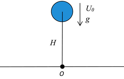
FIGURE 1. Schematic diagram of the droplet impacting the horizontal solid wall.

Here, the Newtonian droplet is considered to be two-dimensional, and its initial diameter and velocity are $D=0.02\mathrm{m}$ and $U_0=-1{\mathrm{m}\mathrm{s}}^{-1}$, respectively. The center of the droplet is initially at position $\left(0.0,0.0\right)$ with the height $H=0.04\mathrm{m}$ to the horizontal rigid wall. The initial particle spacing is set to $d_0=0.0004\mathrm{m}$, and the time-step is set to $\Delta t=1\times {10}^{-5}\mathrm{s}$. The gravitational acceleration acts downward with $g=-9.81{\mathrm{m}\mathrm{s}}^{-2}$. The reference density is ${\rho }_0={10}^3{\mathrm{k}\mathrm{g}\mathrm{m}}^{-3}$, the total viscosity is $\eta =4\mathrm{P}\mathrm{a}\cdot \mathrm{s}$, and the speed of sound is $c=12.5{\mathrm{m}\mathrm{s}}^{-1}$. The artificial viscosity parameter ${\alpha }_{\Pi }=1.0$ and ${\beta }_{\Pi }=2.0$. The droplet contains $\mathrm{1,961}$ fluid particles, and the solid wall consists of $251$ wall particles and $753$ ghost particles.

Figure 2 shows the symmetrical evolution process of Newtonian droplets along the wall after impacting. The figures show that the droplet surface evolves smoothly, indicating good numerical stability. For the evolution of the droplet width with dimensionless time, Figure 3 shows a comparison of numerical results obtained using the SPH and CSPH methods. The dimensionless time is $t^{*}=\left(U/L\right)t$, where $U=\left|U_0\right|$ and $L=H$. For ease of expression, the dimensionless time in the study is still recorded as $t$. Figure 3 shows that the result using CSPH is closer to the result by Tomé et al. (2002) compared to that using SPH. Thus, the results obtained by the CSPH method are more accurate than those obtained by the SPH method.

FIGURE 2

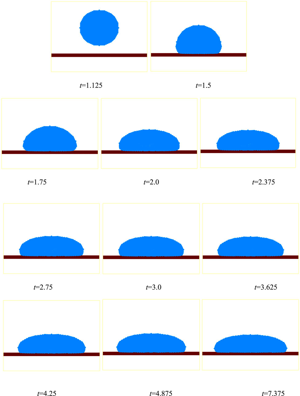
FIGURE 2. Evolution process of the Newtonian droplet impacting the horizontal solid wall.

FIGURE 3

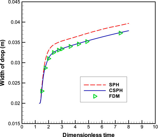
FIGURE 3. Comparison of droplet widths calculated using SPH and CSPH (the FDM result is obtained by Tome et al.).

The tension instability occurs in the numerical simulations of Newtonian and Bingham fluids using the traditional SPH method, which leads to particle clustering or fractal phenomenon. The influence of tension instability on the numerical simulation of Bingham fluid is more serious than that of the Newtonian fluid. In order to solve this problem, the CSPH method in this study adds the artificial stress item. Figure 4 shows the numerical results of the Bingham droplet impacting the solid wall using the traditional SPH and CSPH methods. For the Bingham model, ${\mu }_B=4\times {10}^{-4}{\mathrm{m}}^2{\mathrm{s}}^{-1}$, ${\tau }_y=3.6\times {10}^{-3}\mathrm{P}\mathrm{a}$, and the other parameter values are the same as those in the Newtonian fluid. Figure 4Ashows that due to the tension instability, the fluid particles show serious clustering and fractal phenomena in the numerical simulation of Bingham liquid drops hitting the solid wall with the traditional SPH method. Although Figure 4B shows no obvious fluid particle clustering and fractal phenomenon, the fluid particles are evenly distributed, and the droplet surface is smooth during the simulation of Bingham droplet impacting the solid wall with the CSPH method. Thus, the CSPH method can overcome the problem of tension instability well.

FIGURE 4

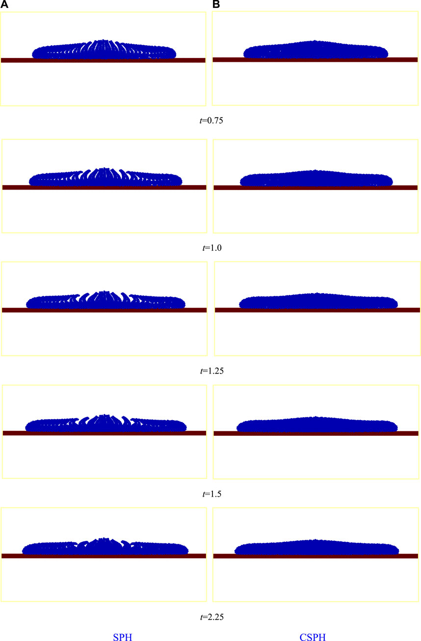
FIGURE 4. Bingham droplet impacting the horizontal solid wall with SPH and CSPH: (A) SPH and (B) CSPH.

4.2 Numerical simulation of the Bingham fluid flow on a slope

This section considers the flow characteristics of Bingham fluid on a slope under the action of gravity. The flow process of the corresponding Newtonian case is also considered for comparison. In addition, the influence of slope angle on the flow behavior of the Bingham fluid is analyzed.

Figure 5 shows the schematic diagrams of fluid flow on a slope with an inclination angle α. For simplicity, the initial state of the fluid on the slope is a semicircle with the center of the circle at the origin $O\left(0,0\right)$ on the slope, as shown in Figure 5A. The fluid flows down the slope under the action of gravity, as shown in Figure 5B.

FIGURE 5

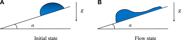
FIGURE 5. Schematic diagram of fluid flow on a slope: (A) initial state and (B) flow state.

4.2.1 Fluids flow on a slope with Bingham and Newtonian models

The initial state of the fluid is shown in Figure 5A. In this state, the diameter of the semicircle is $D=0.04\mathrm{m}$ and the inclination angle is $\alpha ={45}^{\circ }$. In addition to the flow evolution process of the Bingham fluid on the slope, the corresponding Newtonian case is also shown in this section for comparison. For the Bingham model, ${\mu }_B=4\times {10}^{-4}{\mathrm{m}}^2{\mathrm{s}}^{-1}$ and ${\tau }_y=3.6\times {10}^{-3}\mathrm{P}\mathrm{a}$. Generally, the density of the Bingham fluid is larger than that of water. Here, in order to compare the fluid flow behaviors described by the Bingham and Newtonian models, the same reference density ${\rho }_0={10}^3{\mathrm{k}\mathrm{g}\mathrm{m}}^{-3}$ is adopted for both, and the other parameter values are the same as those in the case of the Newtonian fluid. Namely, the number of fluid particles is 3,852, the number of wall particles is 501, and the number of ghost particles is 1,503. The initial spacing $d_0=0.0004\mathrm{m}$, and the time-step $\Delta t=1\times {10}^{-5}\mathrm{s}$. The gravitational acceleration is $g=-9.81{\mathrm{m}\mathrm{s}}^{-2}$, and the speed of sound is $c=10{\mathrm{m}\mathrm{s}}^{-1}$. The artificial viscosity parameter ${\alpha }_{\Pi }=1.0$ and ${\beta }_{\Pi }=2.0$. In addition, the Newtonian fluid has the changeless total viscosity $\eta =4\mathrm{P}\mathrm{a}\cdot \mathrm{s}$.

Figures 6A,B show the flow evolution process on a slope for Newtonian and Bingham fluids, respectively. A comparison of the two cases shows that the flow deformation of the Bingham fluid is more obvious than that in the Newtonian case. Besides, the flow velocity of the Bingham fluid is larger than that in the Newtonian case (see Figures 7, 8). Here, the frontmost particle velocity and the front average velocity are calculated to describe the flow velocity. The frontmost particle velocity refers to the velocity of the particle in the forefront of fluid, and the front average velocity refers to the statistical average of the velocities of some particles in the flow front. These flow characteristics of the Bingham fluid are the manifestation of a shear thinning behavior. Figure 6B shows that the Bingham fluid flow develops into a multi-crest pattern, similar to the intermittent flow. As shown in Figure 7, the flow rate of the Newtonian fluid reaches the peak at about t = 1.8, whereas that of the Bingham fluid reaches the peak at about t = 2.5. Subsequently, as the mass of the front fluid decreases, the influence of viscous resistance on the slope surface becomes obvious, and the velocity decreases gradually. Figure 9 shows that the frontmost particle velocity is higher than the front average velocity because the bottom particles are affected by the viscous resistance of the slope surface, which reduces the front average velocity.

FIGURE 6

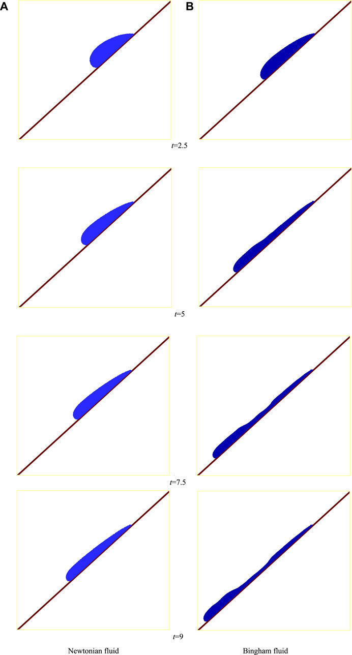
FIGURE 6. Fluid flow on a slope: (A) Newtonian fluid and (B) Bingham fluid.

FIGURE 7

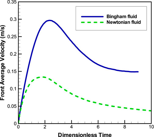
FIGURE 7. Front average velocity.

FIGURE 8

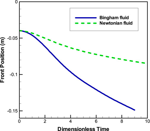
FIGURE 8. Front position of the x direction.

FIGURE 9

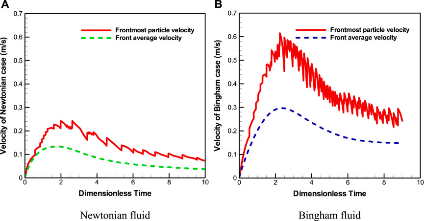
FIGURE 9. Velocity: (A) Newtonian fluid and (B) Bingham fluid.

4.2.2 Fluid flow on a slope with different tilt angles

The steepness of the slope will have a significant effect on the flow behavior of the Bingham fluid. In order to test the ability of CSPH simulation under a wide range of inclination angles and analyze the flow characteristics of the Bingham fluid on slopes with different inclination angles, the CSPH method is used to simulate the flow process of the Bingham fluid on the slopes with inclination angles of 30^o, 50^o, and 60^o, respectively. Here, the reference density of the Bingham fluid is taken as $\rho =1100{\mathrm{k}\mathrm{g}\mathrm{m}}^{-3}$, and the other physical parameter values are the same as those in Section 4.2.1.

Figures 10–12 show the flow characteristics of the Bingham fluid at different tilt angles (α=30^o, 50^o, 60^o), and Figure 13 shows their front average velocity. The figures show that the fluid accumulation in front becomes more obvious with the tilt angle enlarging. The accumulation changes the fluid flow behavior. When the fluid accumulation in front is small, the viscous force on the slope surface greatly influences the flow, and the front flow velocity is small. In this case, as the slope surface that the fluid has flowed through has been wetted, the viscous resistance of the slope surface behind the fluid front is reduced, and the subsequent fluid gradually catches up and accumulates in front. When the front fluid accumulates to a certain amount, the volume force increases to a sufficient degree and plays a leading role and the influence of slope viscous resistance decreases. Thus, the front fluid accelerates to flow forward and distances itself from the fluid behind, which forms a multi-crest flow pattern (see Figure 11C). As the front fluid flows forward, fluid adhesion on the slope surface leads to fluid loss in the front. Thus, the volume force of the front fluid decreases, and the influence of viscous resistance on the slope surface increases, leading to the front velocity decrease. Under the lubrication of the slope surface, the rear crests catch up with the front crest and overlap (see Figures 11C, 12C). The downward flow of the Bingham fluid on a slope is a competition process between gravity and viscous friction. In the case of a small slope, viscous friction plays a dominant role, and in the case of large slopes, gravity plays a dominant role, resulting in different flow patterns at different slopes.

FIGURE 10

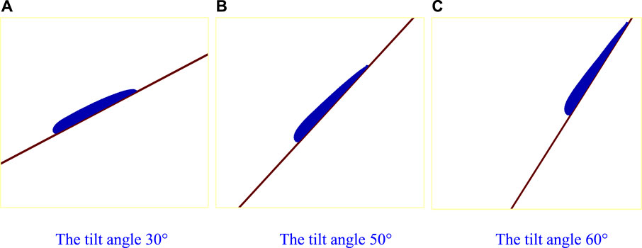
FIGURE 10. Bingham fluid flow on a slope at t = 3.75 with tilt angles of 30°, 50°, and 60°. (A) The tilt angle of 30°. (B) The tilt angle of 50°. (C) The tilt angle of 60°.

FIGURE 11

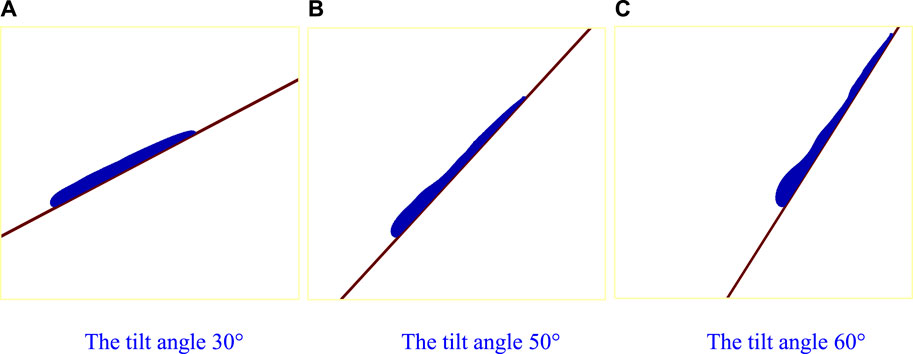
FIGURE 11. Bingham fluid flow on a slope at t = 5.75 with tilt angles of 30°, 50°, and 60°. (A) The tilt angle of 30°. (B) The tilt angle of 50°. (C) The tilt angle of 60°.

FIGURE 12

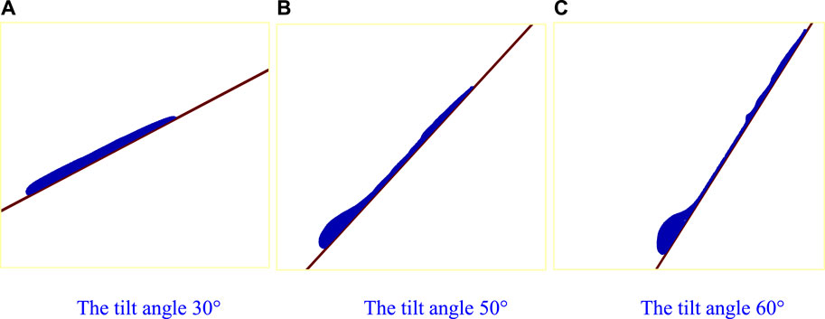
FIGURE 12. Bingham fluid flow on a slope at t = 8.5 with tilt angles of 30°, 50°, and 60°. (A) The tilt angle of 30°. (B) The tilt angle of 50°. (C) The tilt angle of 60°.

FIGURE 13

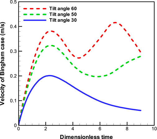
FIGURE 13. The front average velocity of Bingham fluid flow on a slope with the tilt angles of 30°, 50°, and 60°.

5 Conclusion

To understand the motion characteristics of viscoplastic fluid, we introduced the improved SPH method to investigate the flow process of the Bingham fluid on a slope in this study. Firstly, we add the artificial stress term to the momentum equation to relieve the tension instability. Consequently, the SPH method based on the periodic re-initialization of density is improved to keep the consistency between mass, density, and occupied volume. The higher accuracy and stability of the improved SPH method are validated by droplet examples of Newtonian and Bingham fluids. Secondly, we numerically investigate the flow characteristic of the Bingham fluid on a slope using the improved SPH method and compare the results to those of the Newtonian case. The computational results show that the corrected SPH method can accurately simulate the rheological behavior of the Bingham fluid, such as shear thinning. Furthermore, the numerical results with a large range of incline angles are given to prove the effectiveness and stability of the improved SPH method, which can effectively capture the complex transient flow behavior of Bingham fluid and be applied to large-scale and real scene debris flow numerical simulation with parallel technology.

Data availability statement

The original contributions presented in the study are included in the article/supplementary material. Further inquiries can be directed to the corresponding author.

Author contributions

All authors listed have made a substantial, direct, and intellectual contribution to the work and approved it for publication.

Funding

The National Natural Science Foundation of China (no. 61962051) and the National Natural Science Foundation of China (no. 12161058). This research was funded by the National Natural Science Foundation of China (No. 61962051), the Open Project of State Key Laboratory of Plateau Ecology and Agriculture, Qinghai University (No. 2021-ZZ-02), the Jiangxi Provincial Natural Science Foundation (No. 20212BAB201020), the National Natural Science Foundation of China (No. 12161058), the Jiangxi Provincial Education Department (No. GJJ190961), the Youth Foundation Program of Qinghai University (No. 2020-QGY-11), and the Chunhui project of the Ministry of Education (No. QDCH2018001).

Conflict of interest

The authors declare that the research was conducted in the absence of any commercial or financial relationships that could be construed as a potential conflict of interest.

Publisher’s note

All claims expressed in this article are solely those of the authors and do not necessarily represent those of their affiliated organizations or those of the publisher, the editors, and the reviewers. Any product that may be evaluated in this article, or claim that may be made by its manufacturer, is not guaranteed or endorsed by the publisher.

References

Benz, W. (1990). Smooth particle hydrodynamics: A review. The Numerical Modelling of Nonlinear Stellar Pulsations. Heidelberg: Springer, 269–288.

CrossRef Full Text | Google Scholar

Canelas, R. B., Domínguez, J. M., Crespo, A. J. C., Gómez-Gesteira, M., and Rui, M. L. F. (2015). A Smooth Particle Hydrodynamics discretization for the modelling of free surface flows and rigid body dynamics. Int. J. Numer. Methods Fluids 78 (9), 581–593. doi:10.1002/fld.4031

CrossRef Full Text | Google Scholar

Chen, H., and Lee, C. F. (2002). Runout analysis of slurry flows with bingham model. J. Geotech. Geoenviron. Eng. 128 (12), 1032–1042. doi:10.1061/(asce)1090-0241(2002)128:12(1032)

CrossRef Full Text | Google Scholar

Chen, J. K., and Beraun, J. E. (2000). A generalized smoothed particle hydrodynamics method for nonlinear dynamic problems. Comput. Methods Appl. Mech. Eng. 190 (1-2), 225–239. doi:10.1016/s0045-7825(99)00422-3

CrossRef Full Text | Google Scholar

Chen, Y., Qiu, Z., Li, B., and Yang, Z. (2018). Numerical simulation on the dynamic characteristics of a tremendous debris flow in sichuan, China. Process. (Basel). 6 (8), 109. doi:10.3390/pr6080109

CrossRef Full Text | Google Scholar

De Blasio, F. V., Elverhøi, A., Issler, D., Harbitz, C. B., Bryn, P., and Lien, R. (2004). Flow models of natural debris flows originating from overconsolidated clay materials. Mar. Geol. 213 (1-4), 439–455. doi:10.1016/j.margeo.2004.10.018

CrossRef Full Text | Google Scholar

Fang, J., Owens, R. G., Tacher, L., and Parriaux, A. (2006). A numerical study of the SPH method for simulating transient viscoelastic free surface flows. J. Newt. Fluid Mech. 139 (1-2), 68–84. doi:10.1016/j.jnnfm.2006.07.004

CrossRef Full Text | Google Scholar

Fang, J., Parriaux, A., Rentschler, M., and Ancey, C. (2009). Improved SPH methods for simulating free surface flows of viscous fluids. Appl. Numer. Math. 59 (2), 251–271. doi:10.1016/j.apnum.2008.02.003

CrossRef Full Text | Google Scholar

Gray, J. P., Monaghan, J. J., and Swift, R. P. (2001). SPH elastic dynamics. Comput. Methods Appl. Mech. Eng. 190 (49-50), 6641–6662. doi:10.1016/s0045-7825(01)00254-7

CrossRef Full Text | Google Scholar

Huang, C., Lei, J. M., Liu, M. B., and Peng, X. Y. (2015). A kernel gradient free (KGF) SPH method. Int. J. Numer. Methods Fluids 78, 691–707. doi:10.1002/fld.4037

CrossRef Full Text | Google Scholar

Huang, Y., Cheng, H., Dai, Z., Xu, Q., Liu, F., Sawada, K., et al. (2015). SPH-based numerical simulation of catastrophic debris flows after the 2008 Wenchuan earthquake. Bull. Eng. Geol. Environ. 74 (4), 1137–1151. doi:10.1007/s10064-014-0705-6

CrossRef Full Text | Google Scholar

Huang, Y., Zhang, W., Mao, W., and Jin, C. (2011). Flow analysis of liquefied soils based on smoothed particle hydrodynamics. Nat. Hazards (Dordr). 59 (3), 1547–1560. doi:10.1007/s11069-011-9851-3

CrossRef Full Text | Google Scholar

Lind, S. J., Stansby, P. K., Rogers, B. D., and Lloyd, P. M. (2015). Numerical predictions of water-air wave slam using incompressible-compressible smoothed particle hydrodynamics. Appl. Ocean Res. 49, 57–71. doi:10.1016/j.apor.2014.11.001

CrossRef Full Text | Google Scholar

Liu, M. B., and Liu, G. R. (2006). Restoring particle consistency in smoothed particle hydrodynamics. Appl. Numer. Math. 56 (1), 19–36. doi:10.1016/j.apnum.2005.02.012

CrossRef Full Text | Google Scholar

Mahmood, R., Kousar, N., Usman, K., and Mehmood, A. (2018). Finite element simulations for stationary Bingham fluid flow past a circular cylinder. J. Braz. Soc. Mech. Sci. Eng. 40 (9), 459. doi:10.1007/s40430-018-1383-2

CrossRef Full Text | Google Scholar

Mahmood, R., Kousar, N., Yaqub, M., and Jabeen, K. (2017). Numerical simulations of the square lid driven cavity flow of bingham fluids using nonconforming finite elements coupled with a direct solver. Adv. Math. Phys. 2017, 1–10. doi:10.1155/2017/5210708

CrossRef Full Text | Google Scholar

Monaghan, J. J. (1994). Simulating free surface flows with SPH. J. Comput. Phys. 110 (2), 399–406. doi:10.1006/jcph.1994.1034

CrossRef Full Text | Google Scholar

Monaghan, J. J. (1992). Smoothed particle hydrodynamics. Annu. Rev. Astron. Astrophys. 30 (1), 543–574. doi:10.1146/annurev.aa.30.090192.002551

CrossRef Full Text | Google Scholar

Monaghan, J. J. (2005). Smoothed particle hydrodynamics. Rep. Prog. Phys. 68 (8), 1703–1759. doi:10.1088/0034-4885/68/8/r01

CrossRef Full Text | Google Scholar

Monaghan, J. J. (2000). SPH without a tensile instability. J. Comput. Phys. 159 (2), 290–311. doi:10.1006/jcph.2000.6439

CrossRef Full Text | Google Scholar

Moreno, E., Dialami, N., and Cervera, M. (2021). Modeling of spillage and debris floods as Newtonian and Viscoplastic Bingham flows with free surface with mixed stabilized finite elements. J. Newt. Fluid Mech. 290 (2), 104512. doi:10.1016/j.jnnfm.2021.104512

CrossRef Full Text | Google Scholar

Morris, J. P., Fox, P. J., and Zhu, Y. (1997). Modeling low Reynolds number incompressible flows using SPH. J. Comput. Phys. 136 (1), 214–226. doi:10.1006/jcph.1997.5776

CrossRef Full Text | Google Scholar

Olshanskii, M. A. (2009). Analysis of semi-staggered finite-difference method with application to Bingham flows. Comput. Methods Appl. Mech. Eng. 198 (9-12), 975–985. doi:10.1016/j.cma.2008.11.010

CrossRef Full Text | Google Scholar

Ren, B., Wen, H., Dong, P., and Wang, Y. (2014). Numerical simulation of wave interaction with porous structures using an improved smoothed particle hydrodynamic method. Coast. Eng. 88, 88–100. doi:10.1016/j.coastaleng.2014.02.006

CrossRef Full Text | Google Scholar

Roquet, N., and Saramito, P. (2003). An adaptive finite element method for Bingham fluid flows around a cylinder. Comput. Methods Appl. Mech. Eng. 192 (31-32), 3317–3341. doi:10.1016/s0045-7825(03)00262-7

CrossRef Full Text | Google Scholar

Shao, S., and Gotoh, H. (2005). Turbulence particle models for tracking free surfaces. J. Hydraulic Res. 43 (3), 276–289. doi:10.1080/00221680509500122

CrossRef Full Text | Google Scholar

Shao, S. (2011). Incompressible smoothed particle hydrodynamics simulation of multifluid flows. Int. J. Numer. Methods Fluids 69 (11), 1715–1735. doi:10.1002/fld.2660

CrossRef Full Text | Google Scholar

Shao, S. (2010). Incompressible SPH flow model for wave interactions with porous media. Coast. Eng. 57 (3), 304–316. doi:10.1016/j.coastaleng.2009.10.012

CrossRef Full Text | Google Scholar

Shao, S., Ji, C., Graham, D. I., Reeve, D. E., James, P. W., and Chadwick, A. J. (2006). Simulation of wave overtopping by an incompressible SPH model. Coast. Eng. 53 (9), 723–735. doi:10.1016/j.coastaleng.2006.02.005

CrossRef Full Text | Google Scholar

Swegle, J. W., Hicks, D. L., and Attaway, S. W. (1995). Smoothed particle hydrodynamics stability analysis. J. Comput. Phys. 116 (1), 123–134. doi:10.1006/jcph.1995.1010

CrossRef Full Text | Google Scholar

Tomé, M. F., Mangiavacchi, N., Cuminato, J. A., Castelo, A., and McKee, S. (2002). A finite difference technique for simulating unsteady viscoelastic free surface flows. J. Newt. Fluid Mech. 106 (2-3), 61–106. doi:10.1016/s0377-0257(02)00064-2

CrossRef Full Text | Google Scholar

Uzuoka, R., Yashima, A., Kawakami, T., and Konrad, J.-M. (1998). Fluid dynamics based prediction of liquefaction induced lateral spreading. Comput. Geotechnics 22 (3-4), 243–282. doi:10.1016/s0266-352x(98)00006-8

CrossRef Full Text | Google Scholar

Wang, W., Chen, G., Han, Z., Zhou, S., Zhang, H., and Jing, P. (2016). 3D numerical simulation of debris-flow motion using SPH method incorporating non-Newtonian fluid behavior. Nat. Hazards (Dordr). 81 (3), 1981–1998. doi:10.1007/s11069-016-2171-x

CrossRef Full Text | Google Scholar

Wang, Z., Yu, X., Zhang, W., Zhang, F., Zhou, Y., and Gao, Y. (2019). SPH-based analysis on the lateral response of pipe culverts in the flowing process of liquefied sand. Math. Problems Eng. 2019, 43515011–43515012. doi:10.1155/2019/4351501

CrossRef Full Text | Google Scholar

Wen, H., Ren, B., Dong, P., and Zhu, G. (2020). Numerical analysis of wave-induced current within the inhomogeneous coral reef using a refined SPH model. Coast. Eng. 156, 103616. doi:10.1016/j.coastaleng.2019.103616

CrossRef Full Text | Google Scholar

Wen, H., Ren, B., and Yu, X. (2018). An improved SPH model for turbulent hydrodynamics of a 2D oscillating water chamber. Ocean. Eng. 150, 152–166. doi:10.1016/j.oceaneng.2017.12.047

CrossRef Full Text | Google Scholar

Whipple, K. X. (1997). Open-channel flow of bingham fluids: Applications in debris-flow research. J. Geol. 105 (2), 243–262. doi:10.1086/515916

CrossRef Full Text | Google Scholar

Wu, H., He, N., and Zhang, X. (2015). Numerical model of viscous debris flows with depth-dependent yield strength. J. Geoengin. 10 (1), 1–10.

Google Scholar

Ye, C., Mota, P., Li, J., Lin, K., and Qian, W.-L. (2019). On the boundary condition and related instability in the smoothed particle hydrodynamics. Commun. Theor. Phys. 11, 1281–1292. doi:10.1088/0253-6102/71/11/1281

CrossRef Full Text | Google Scholar

Zhao, Z., Ouyang, J., Zhang, L., and Liu, D. (2008). Numerical simulation of branched polymer melts through planar contraction with inset based on XPP model. J. Chem. Industry Eng. 59 (4), 843–850.

Google Scholar

Zheng, S., Ouyang, J., Zhang, L., and Zhang, H. (2007). Dynamic simulation of fusion process and analysis of flow field. J. Reinf. Plastics Compos. 26 (17), 1781–1792. doi:10.1177/0731684407080479

CrossRef Full Text | Google Scholar

Zheng, S., Ouyang, J., Zhang, L., and Zhao, Z. (2009). Research on a numerical schemes for capturing free front during injection molding. Polymer-Plastics Technol. Eng. 48 (4), 446–454. doi:10.1080/03602550902725456

CrossRef Full Text | Google Scholar

Zhu, H., Martys, N. S., Ferraris, C., and Kee, D. D. (2010). A numerical study of the flow of Bingham-like fluids in two-dimensional vane and cylinder rheometers using a smoothed particle hydrodynamics (SPH) based method. J. Newt. Fluid Mech. 165 (7-8), 362–375. doi:10.1016/j.jnnfm.2010.01.012

CrossRef Full Text | Google Scholar