CEA-FJSP: Carbon emission-aware flexible job-shop scheduling based on deep reinforcement learning

Currently, excessive carbon emission is causing visible damage to the ecosystem and will lead to long-term environmental degradation in the future. The manufacturing industry is one of the main contributors to the carbon emission problem. Therefore, the reduction of carbon emissions should be considered at all levels of production activities. In this paper, the carbon emission as a parvenu indicator is considered parallelly with the nobleman indicator, makespan, in the flexible job-shop scheduling problem. Firstly, the carbon emission is modeled based on the energy consumption of machine operation and the coolant treatment during the production process. Then, a deep reinforcement learning-based scheduling model is proposed to handle the carbon emission-aware flexible job-shop scheduling problem. The proposed model treats scheduling as a Markov decision process, where the scheduling agent and the scheduling environment interact repeatedly via states, actions, and rewards. Next, a deep neural network is employed to parameterize the scheduling policy. Then, the proximal policy optimization algorithm is conducted to drive the deep neural network to learn the objective-oriented optimal mapping from the states to the actions. The experimental results verify that the proposed deep reinforcement learning-based scheduling model has prominent optimization and generalization abilities. Moreover, the proposed model presents a nonlinear optimization effect over the weight combinations.

1 Introduction

Production scheduling is a subclass of combinational optimization problems aiming to sequence jobs to machines toward the optimization of one or more scheduling objectives (Fernandes et al., 2022). Production scheduling can be classified into many types according to its inherent properties. For example, the job-shop scheduling problem (JSSP) specifies that one operation can only be processed by one machine (Zhang et al., 2019), while the flexible job-shop scheduling problem (FJSP) allows multiple candidate machines to process an operation (Brucker and Schlie, 1990). The frequently adopted scheduling objectives related to economic benefits include makespan, tardiness, and machine utilization (Allahverdi et al., 2008). In recent years, the steady deterioration of environmental problems (Bhatti et al., 2021; Bhatti et al., 2022a; Bhatti et al., 2022b), such as pollution and climate change, has raised the awareness of environmental protection. Hence, environmental indicators, especially energy consumption and carbon emission, are a growing concern in production scheduling (Gao et al., 2020). Therefore, the FJSP is formulated as a multi-objective optimization problem considering both economic benefit and environmental effect.

The heuristic and meta-heuristic algorithms have been widely applied to achieve multi-objective scheduling. In terms of heuristic algorithms, Zhang et al. (2022) proposed a greedy algorithm and an elite strategy to solve FJSP with the objectives of minimizing both makespan and total energy consumption. Xu et al. (2021) proposed three delayed routing strategies to optimize energy efficiency and mean tardiness in dynamic FJSP. In terms of meta-heuristic algorithms, the multi-objective genetic algorithm (GA) is the most popular scheme due to its excellent global optimization ability and convergence performance (Li and Wang, 2022). Several GA-based algorithms have been proposed to improve search efficiency for minimizing makespan and total energy consumption (Mokhtari and Hasani, 2017; Dai et al., 2019) and to determine machine start/stop time and speed level to save energy (Wu and Sun, 2018). Moreover, none-GA based algorithms including the frog-leaping algorithm (Lei et al., 2017) and the grey wolf algorithm (Luo et al., 2019) are also available for multi-objective scheduling.

However, the above-mentioned scheduling algorithms lack generalization ability (Han and Yang, 2021). To solve an FJSP instance that is different from the solved ones in terms of parameters such as the number of jobs and machines, the existing heuristic algorithms generally require the development of new scheduling rules while the meta-heuristic algorithms require considerable iterative computation time to obtain high-quality scheduling solutions. In contrast, deep reinforcement learning (DRL) based (Arulkumaran et al., 2017) production scheduling can learn and generalize the knowledge from the training samples to new problems. Therefore, the trained DRL models can be applied to different scheduling scenarios to produce satisfactory scheduling solutions in a reasonable computation time. Qu et al. (2016) and van Ekeris et al. (2021) stated that DRL could discover basic heuristic behaviors for production scheduling from scratch, providing a kind of optimization-capable, scalable, and real-time scheduling methods.

Numerous studies have utilized the generalization ability of DRL to solve different-scale production scheduling problems (Ren et al., 2020; Zhang et al., 2020; Monaci et al., 2021; Ni et al., 2021; Park et al., 2021). However, these studies focused on either the single objective JSSP (Han and Yang, 2020; Liu et al., 2020; Zhao et al., 2021; Zeng et al., 2022) or the flow-shop scheduling problem (FSSP) (Pan et al., 2021; Yan et al., 2022). The multi-objective FJSPs have been seldom addressed (Lang et al., 2020; Luo et al., 2021). Furthermore, among the few studies addressing the DRL-based multi-objective FJSP, even fewer studies cared about environmental objectives (Naimi et al., 2021; Du et al., 2022). Therefore, the development of DRL-based methods for solving FJSP is still in the initial stage and not yet systematic (Luo, 2020; Feng et al., 2021; Liu et al., 2022).

In summary, the existing DRL-based methods for FJSP receive less attention compared with those for JSSP. Moreover, most of the studies preferred the optimization of single or multiple economic objectives to the optimization of environmental objectives. Although some studies have attempted to minimize total energy consumption or electricity cost, minimizing carbon emissions has not been yet explicitly considered. Furthermore, a few studies integrated a DRL model with a meta-heuristic algorithm to solve the multi-objective FJSP. However, the DRL model was used as an auxiliary tool to assist the meta-heuristic algorithm to improve search efficiency. To resolve the above-mentioned technical limitation, this paper proposes a DRL-based scheduling method to handle FJSP to minimize both makespan and total carbon emission. The main contributions of this study are listed as follows.

1) The classical FJSP is extended to a carbon emission-aware flexible job-shop scheduling problem (CEA-FJSP), where a carbon emission accounting model is formulated based on the energy consumption of machine operation and coolant treatment during the production process.

2) An intelligent DRL-based scheduling model is developed to directly generate feasible scheduling solutions for CEA-FJSP without extra searching. The solving process is modeled as a Markov decision process (MDP) including generic productive state features, a scheduling rule-based action space, and a composite reward function.

3) The scheduling policy is parameterized by a deep neural network (DNN), that is, optimized by the proximal policy optimization (PPO) algorithm to establish the mapping from the states to the actions.

4) The experimental results on various benchmarks demonstrate that the proposed DRL scheduling model has prominent optimization and generalization abilities. Moreover, the proposed model presents a nonlinear optimization effect over the weight combinations.

The remainder of this paper is organized as follows. The mathematical model of the CEA-FJSP is formulated in Section 2. The DRL scheduling model is described in Section 3. Section 4 presents the experimental results and Section 5 concludes the study.

2 Problem formulation

This section mathematically describes the conditions and constraints of the CEA-FJSP. There are $n$ jobs belonging to a job set $\mathcal{I}=\left\{J_1,J_2,\dots ,J_n\right\}$ to be processed by $m$ machines belonging to a machine set $\mathcal{M}=\left\{M_1,M_2,\dots ,M_m\right\}$. A job $J_i$ consists of $n_i$ operations, where $O_{ij}$ denotes the $j$ th operation of $J_i$. The operations of the same job $J_i$ must be processed in a specific order, i.e., $O_{i1}\to O_{i2}\cdots \to O_{i{n}_i}$. The operation $O_{ij}$ can be processed by one or more machines forming an operation-specific candidate machine set ${\mathcal{M}}_{ij}\subseteq \mathcal{M}$. The time and the power that the machine $M_k\in {\mathcal{M}}_{ij}$ requires to process the operation $O_{ij}$ are denoted as $t_{ijk}$ and $p_{ijk}$, respectively. The machine $M_k$ also requires coolant during processing and constant lower power consumption in an idle state. The scheduling for CEA-FJSP aims to obtain an optimal scheduling solution to minimize both makespan and carbon emission, by determining a machine $M_k$ from ${\mathcal{M}}_{ij}$, the start time $S_{ij}$, and the completion time $C_{ij}=S_{ij}+t_{ijk}$ for each operation $O_{ij}$. Furthermore, the following constraints and assumptions should be satisfied:

1) The operations of the same job should be processed following the defined operation precedence.

2) A machine can only process one operation at a time.

3) An operation should be processed without interruption.

4) A machine processes an operation with constant processing power.

5) All machines turn on at the start of the scheduling.

6) The transportation time of jobs and the setup time of machines are negligible.

Based on the above description, a carbon emission accounting model is formulated firstly to identify the main sources and specific computation of carbon emission in CEA-FJSP. Then, the mathematical model of the CEA-FJSP is established. Table 1 lists the notations used in the models.

TABLE 1

TABLE 1. Notations for CEA-FJSP.

2.1 Carbon emission accounting model

Carbon emission is produced directly or indirectly by various manufacturing links, such as raw materials consumption, machine operation, transportation, and metal debris treatment (Gutowski et al., 2005). In this paper, the electrical energy consumption of machine operation and the energy consumption of coolant treatment are identified as the main carbon emission sources in CEA-FJSP.

2.1.1 Carbon emission from machine operation

Generally, a machine experiences five working modes in a duty cycle: start-up, warm-up, processing, idle, and stop. Each mode requires a different power level as shown in Figure 1. The modes of start-up, warm-up, and stop appear only once in a duty cycle and the energy consumption in these modes is only related to machine properties rather than scheduling. In contrast, the processing and idle modes tend to alternately appear multiple times. Therefore, only the carbon emission in processing and idle modes are considered in scheduling.

FIGURE 1

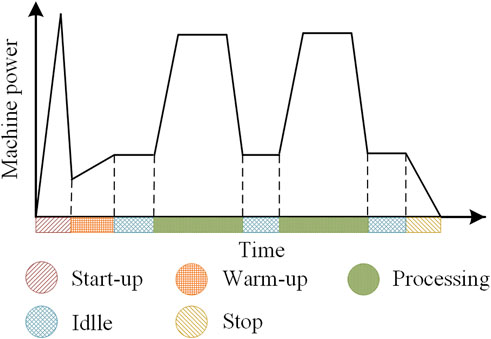
FIGURE 1. Power variation of five machine working modes.

Under processing mode, the carbon emission ${CE}_p$ is calculated as:

$\begin{array}{c}{CE}_p={\alpha }_e{W}_p\end{array}(1)$

where $W_p$ is the total electrical energy consumption of all machines under processing mode and is expressed as:

$\begin{array}{c}{W}_p={\displaystyle \sum }_{k=1}^m{\displaystyle \sum }_{i=1}^n{\displaystyle \sum }_{j=1}^{n_i}{x}_{ijk}{p}_{ijk}{t}_{ijk}\end{array}(2)$

Under idle mode, the carbon emission ${CE}_r$ is calculated as:

$\begin{array}{c}{CE}_r={\alpha }_e{W}_r\end{array}(3)$

where $W_r$ is the total electrical energy consumption of all machines under idle mode and is expressed as:

$\begin{array}{c}{W}_r={\displaystyle \sum }_{k=1}^m{p}_k^{idle}{t}_k^{idle}\end{array}(4)$

2.1.2 Carbon emission from coolant treatment

The coolant is used to reduce the cutting temperature and tool wear and prevent the workpiece from being deformed by heat. The coolant needs to be replaced periodically and the treatment process consumes energy, indirectly producing carbon emissions. To simplify the calculation, it is assumed that the coolant flow rate remains unchanged for the same machine regardless of the processed operations. Hence, the carbon emission of coolant treatment ${CE}_f$ can be calculated as:

$\begin{array}{c}{CE}_f={\alpha }_f{\displaystyle \sum }_{k=1}^m{\displaystyle \sum }_{i=1}^n{\displaystyle \sum }_{j=1}^{n_i}{x}_{ijk}\frac{t_{ijk}}{T_k}{L}_k\end{array}(5)$

The total carbon emission $TCE$ during scheduling adds up as:

$TCE={CE}_p+{CE}_r+{CE}_f\begin{array}{c}={\alpha }_e{\displaystyle \sum }_{k=1}^m{\displaystyle \sum }_{i=1}^n{\displaystyle \sum }_{j=1}^{n_i}{x}_{ijk}{p}_{ijk}{t}_{ijk}+{\alpha }_e{\displaystyle \sum }_{k=1}^m{p}_k^{idle}{t}_k^{idle}+{\alpha }_f{\displaystyle \sum }_{k=1}^m{\displaystyle \sum }_{i=1}^n{\displaystyle \sum }_{j=1}^{n_i}{x}_{ijk}\frac{t_{ijk}}{T_k}{L}_k\end{array}(6)$

2.2 CEA-FJSP formulation

The CEA-FJSP is a multi-objective optimization problem, considering both economic and environmental benefits. The scheduling objectives are to simultaneously minimize $C_{\max }=\max \left\{C_{i{n}_i}|i=\mathrm{1,2},\dots ,n\right\}$ and $TCE$. Therefore, the mathematical model of CEA-FJSP is formulated as:

$\begin{array}{c}\min f=\min \left\{w_1{C}_{\max }+w_{2}TCE\right\}\end{array}(7)$

$\begin{array}{c}s.t.\{\begin{array}{ll}{C}_{\max }\ge C_{ij},\forall i,j& \left(\mathrm{a}\right)\\ C_{ij}=S_{ij}+t_{ijk},S_{ij}\ge 0,\forall i,j,k& \left(\mathrm{b}\right)\\ {\displaystyle \sum }_{M_k\in {\mathcal{M}}_{ij}}{x}_{ijk}=1,\forall i,j& \left(\mathrm{c}\right)\\ S_{i,j+1}\ge C_{ij},\forall i,j& \left(\mathrm{d}\right)\\ C_{i\prime j\prime }-C_{ij}\ge t_{i^{\prime }{j}^{\prime }k},y_{ij{i}^{\prime }{j}^{\prime },k}=1& \left(\mathrm{e}\right)\end{array}\end{array}(8)$

Eq. 7 shows that the objective function minimizes the weighted sum of $C_{\max }$ and $TCE$, converting the multi-objective optimization problem into a single-objective optimization problem, where $w_1$ and $w_2$ are the weights corresponding to $C_{\max }$ and $TCE$, respectively. Eq. 8 shows the five constraints. Constraint (a) in Eq. 8 describes the relationship between makespan and the operation completion time. Constraint (b) ensures that the operation completion time is equal to the sum of the start time and the processing time. Constraint (c) specifies that an operation can be assigned to and processed by only one machine. Constraint (d) guarantees the precedence constraint between the operations of the same job. Constraint (e) shows that a machine can process only one operation at a time.

3 Deep reinforcement learning scheduling modeling

This section proposes a DRL scheduling model for handling CEA-FJSP. Figure 2 shows the framework of the proposed DRL scheduling model. The scheduling environment is an instance of CEA-FJSP initialized with the assumptions and constraints described in Section 2. The scheduling agent embeds a scheduling policy parameterized by a DNN and trained by a DRL algorithm. The agent interacts repeatedly with the environment. In each interaction, the scheduling agent selects an operation and assigns it to a machine, based on the information extracted from the scheduling environment.

FIGURE 2

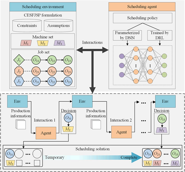
FIGURE 2. Framework of the DRL scheduling model for CEA-FJSP.

The determined operations are queued in a temporary scheduling solution, which is a sequence intuitively describing the precedence of operations. The temporary scheduling solution is turned into a complete and feasible scheduling solution when all operations are determined. Therefore, the scheduling process of a CEA-FJSP instance features an MDP consisting of state, action, and reward. Lastly, the MDP is optimized using a DRL algorithm resulting in a DRL scheduling model.

3.1 Markov decision process formulation

An MDP mainly includes three components: state, action, and reward. A complete decision-making process of MDP is called an episode, consisting of $T={\sum }_{i=1}^n{n}_i$ decision steps in CEA-FJSP, where one decision step corresponds to one interaction. At the decision step $t$, the scheduling agent perceives the state $s_t$ of the scheduling environment. Then, the state features are fed into the scheduling policy that in turn selects an action $a_t$. After the execution of the action $a_t$, an unscheduled operation is selected and assigned to a candidate machine. Hence, the selected operation becomes scheduled. After that, the scheduling environment releases a reward $r_t$ to reflect the change of the scheduling objectives, as well as updates to a new state $s_{t+1}$ ready for the next interaction.

3.1.1 State representation

The state is the basis of decision making and should provide adequate information about the scheduling environment. The number of scheduled operations of job $J_i$ at the decision step $t$ is denoted as ${SO}_i\left(t\right)$. The operations of all the jobs in a scheduling instance are divided into two subsets: ${\mathit{O}}^{\mathit{S}}\left(t\right)=\left\{O_{ij}|1\le i\le n,1\le j\le {SO}_i\left(t\right)\right\}$ and ${\mathit{O}}^{\mathit{U}\mathit{S}}\left(t\right)=\left\{O_{ij}|1\le i\le n,{SO}_i\left(t\right)<j\le n_i\right\}$. Therefore, the completion time $C_{ij}$ can be determined for the operations in the subset ${\mathit{O}}^{\mathit{S}}\left(t\right)$ while the average processing time ${\overline{t}}_{ij}=\underset{M_k\in {\mathcal{M}}_{ij}}{\mathrm{m}\mathrm{e}\mathrm{a}\mathrm{n}}\left(t_{ijk}\right)$ and the average processing power ${\overline{p}}_{ij}=\underset{M_k\in {\mathcal{M}}_{ij}}{\mathrm{m}\mathrm{e}\mathrm{a}\mathrm{n}}\left(p_{ijk}\right)$ can be calculated for the operations in the subset ${\mathit{O}}^{\mathit{U}\mathit{S}}\left(t\right)$.

A statistic-based representation is adopted to define state features using the dynamic attributes of jobs and machines. Table 2 lists the proposed statistic-based state features. It can be seen from the table that the state is a vector consisting of ten features $\left\{f_{t1},f_{t2},\dots ,f_{t10}\right\}$ maintaining a fixed size, which can avoid dimension disaster in large-scale problems. Moreover, the values of the state features are in the range of [0, 1], which can speed up the training process and can be generalized to problems with different configurations.

TABLE 2

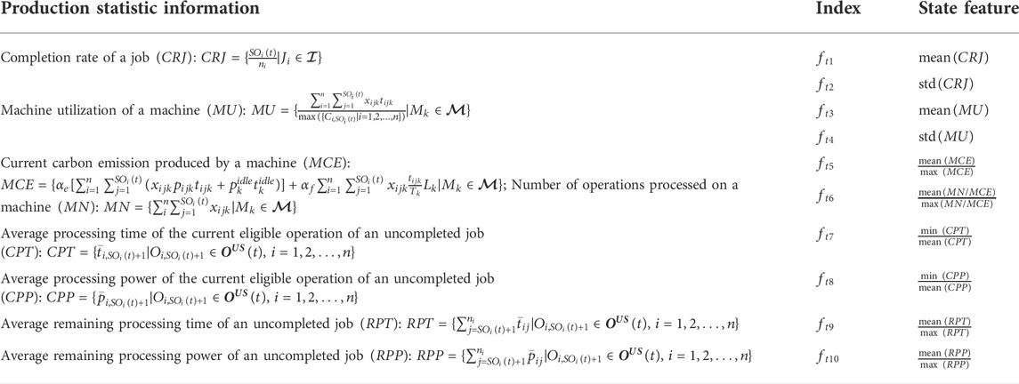
TABLE 2. Statistic-based state features.

3.1.2 Action space

Actions are used to update the scheduling environment, playing a significant role in the quality of scheduling solutions. In the CEA-FJSP, one decision contains two parts: operation selection and machine assignment. Due to the precedence constraint, a job has at most one feasible operation that can be selected at a decision step. Hence, the operation selection can be simplified as the job selection. In this paper, six job selection rules and four machine assignment rules are adopted as shown in Table 3. Nine scheduling rules, $\left\{{SR}_i|i=\mathrm{1,2},\dots ,9\right\}$, are then constructed as follows: ${SR}_1=\left\{\mathrm{J}\mathrm{S}\mathrm{P}\mathrm{T},\mathrm{M}\mathrm{M}\mathrm{A}\mathrm{X}\mathrm{P}\right\}$, ${SR}_2=\left\{\mathrm{J}\mathrm{S}\mathrm{P}\mathrm{T},\mathrm{M}\mathrm{M}\mathrm{I}\mathrm{N}\mathrm{U}\right\}$, ${SR}_3=\left\{\mathrm{J}\mathrm{L}\mathrm{P}\mathrm{T},\mathrm{M}\mathrm{M}\mathrm{A}\mathrm{X}\mathrm{P}\right\}$, ${SR}_4=\left\{\mathrm{J}\mathrm{L}\mathrm{P}\mathrm{T},\mathrm{M}\mathrm{M}\mathrm{I}\mathrm{N}\mathrm{U}\right\}$, ${SR}_5=\left\{\mathrm{J}\mathrm{M}\mathrm{O}\mathrm{R},\mathrm{M}\mathrm{M}\mathrm{I}\mathrm{N}\mathrm{P}\right\}$, ${SR}_6=\left\{\mathrm{J}\mathrm{E}\mathrm{C}\mathrm{T},\mathrm{M}\mathrm{M}\mathrm{A}\mathrm{X}\mathrm{P}\right\}$, ${SR}_7=\left\{\mathrm{J}\mathrm{M}\mathrm{I}\mathrm{N}\mathrm{P},\mathrm{M}\mathrm{M}\mathrm{I}\mathrm{N}\mathrm{U}\right\}$, ${SR}_8=\left\{\mathrm{J}\mathrm{M}\mathrm{I}\mathrm{N}\mathrm{P},\mathrm{M}\mathrm{S}\mathrm{P}\mathrm{T}\right\}$, ${SR}_9=\left\{\mathrm{J}\mathrm{M}\mathrm{A}\mathrm{X}\mathrm{P},\mathrm{M}\mathrm{M}\mathrm{I}\mathrm{N}\mathrm{U}\right\}$. It indicates that a scheduling rule is a couple of a job selection rule and a machine assignment rule. The scheduling rules are called actions in MDP. Thus, the action space consists of nine elements.

TABLE 3

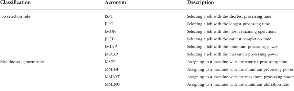
TABLE 3. Job selection and machine assignment rules.

3.1.3 Reward function

As shown in Eq. 7, minimizing $C_{\max }$ and $TCE$ are the two scheduling objectives considered in the CEA-FJSP. However, since the scheduling solution is incomplete during the scheduling, the two performance indicators cannot be resolved until the end of scheduling. In other words, the actual values of $C_{\max }$ and $TCE$ can be calculated only once per episode. Consequently, if the actual makespan and carbon emission values are used as rewards, the immediate reward will be quite sparse and cause difficulties in the convergence of the DRL algorithm.

However, the completion time and carbon emission of the scheduled operations can be used as rewards and determined as:

$\begin{array}{c}{r}_t^{CT}=CT\left(t\right)-CT\left(t+1\right)\end{array}(9)$

$\begin{array}{c}{r}_t^{CE}=CE\left(t\right)-CE\left(t+1\right)\end{array}(10)$

where: $CT\left(t\right)$ is the current maximum completion time of jobs at decision step $t$:

$\begin{array}{c}CT\left(t\right)=\max \left(\left\{C_{i,{SO}_i\left(t\right)}|i=\mathrm{1,2},\dots ,n\right\}\right)\end{array}(11)$

$CE\left(t\right)$ is the currently produced carbon emission at decision step $t$:

$\begin{array}{c}CE\left(t\right)={\alpha }_e\left[{\displaystyle \sum }_{k=1}^m{\displaystyle \sum }_{i=1}^n{\displaystyle \sum }_{j=1}^{{SO}_i\left(t\right)}\left(x_{ijk}{p}_{ijk}{t}_{ijk}+p_k^{idle}{t}_k^{idle}\right)\right]+{\alpha }_f{\displaystyle \sum }_{k=1}^m{\displaystyle \sum }_{i=1}^n{\displaystyle \sum }_{j=1}^{{SO}_i\left(t\right)}{x}_{ijk}\frac{t_{ijk}}{T_k}{L}_k\end{array}(12)$

$r_t^{CT}$ and $r_t^{CE}$ are reward components for makespan and carbon emission, respectively. Therefore, the reward $r_t$ at decision step $t$ is defined according to Eq. 7:

$\begin{array}{c}{r}_t=w_1{r}_t^{CT}+w_2{r}_t^{CE}\end{array}(13)$

To verify Eq. 13, the cumulative reward is calculated as:

$\begin{array}{c}R={\displaystyle \sum }_{t=1}^T{r}_t={\displaystyle \sum }_{t=1}^T\left(w_1{r}_t^{CT}+w_2{r}_t^{CE}\right)\\ ={\displaystyle \sum }_{t=1}^T{w}_1\left(CT\left(t\right)-CT\left(t+1\right)\right)+{\displaystyle \sum }_{t=1}^T{w}_2\left(CE\left(t\right)-CE\left(t+1\right)\right)\\ =w_1\left(CT\left(1\right)-CT\left(T+1\right)\right)+w_2\left(CE\left(1\right)-CE\left(T+1\right)\right)\end{array}(14)$

where $CT\left(1\right)$ and $CE\left(1\right)$ are both zero as none of the operations is determined at the initial step. Once all the operations are determined after the $T$ th decision step, i.e., ${SO}_i\left(T\right)$ is equal to $n_i$, $CT\left(T+1\right)$ and $CE\left(T+1\right)$ are equal to $C_{\max }$ and $TCE$, respectively. Therefore, Eq. 14 can be further simplified as:

$\begin{array}{c}R=-w_{1}CT\left(T+1\right)-w_{2}CE\left(T+1\right)=-\left(w_1{C}_{\max }+w_{2}TCE\right)\end{array}(15)$

Eq. 15 indicates that maximizing the cumulative reward can reach the optimization objectives of minimizing the weighted sum of $C_{\max }$ and $TCE$.

3.2 Policy network

The goal of the scheduling policy is to determine the best-matched action for a given state. In this paper, a DNN with parameter $\theta$ consisting of six fully connected layers is employed to parameterize the scheduling policy denoted as ${\pi }_{\theta }\left(a_t|s_t\right)$. The input layer has ten neurons equal to the number of the state features, and the output layer outputs the probability distribution over the nine actions. Each of the first three hidden layers has sixty-four neurons while the fourth hidden layer has thirty-two neurons, and the Tanh activation function is used for all hidden neurons.

The PPO algorithm is adopted to train the policy network, where the state-value function $V\left(s_t\right)$ is approximated by another DNN with parameter $\varnothing$, denoted as $V_{\varnothing }\left(s_t\right)$. $V_{\varnothing }\left(s_t\right)$ has the same structure as ${\pi }_{\theta }\left(a_t|s_t\right)$ except that the output layer consists of only one neuron, and shares the first three hidden layers with ${\pi }_{\theta }\left(a_t|s_t\right)$ to utilize the learned abstract features.

3.3 Deep reinforcement learning training process

DRL establishes an interaction framework between the agent and the environment using the MDP components: state, action, and reward. The agent learns to optimize its decision-making policy through the interaction, i.e., tunning its policy network ${\pi }_{\theta }\left(a_t|s_t\right)$. Figure 3 illustrates the PPO-based DRL training process for the CEA-FJSP, where a training cycle includes a sampling phase and an update phase. Two same policy networks ${\pi }_{{\theta }_{old}}$ and ${\pi }_{\theta }$ are set-up in the beginning of training to facilitate the training process. During a training cycle, ${\pi }_{{\theta }_{old}}$ remains unchanged throughout the sampling and update phases, while ${\pi }_{\theta }$ is updated multiple times during the update phase.

FIGURE 3

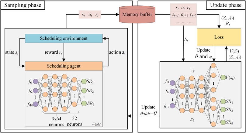
FIGURE 3. PPO-based DRL training process for CEA-FJSP.

In the sampling phase, ${\pi }_{{\theta }_{old}}$ interacts with the scheduling environment to collect sufficient state-action-reward tuples, $\left(s_t,a_t,r_t\right)$, and store into a memory buffer. In the update phase, ${\pi }_{\theta }$ is updated for several epochs with the collected data. After that, ${\pi }_{{\theta }_{old}}$ copies ${\pi }_{\theta }$ and then starts the next training cycle. The surrogate objective loss function of the policy network is defined as:

$\begin{array}{c}{L}_t^{\mathrm{C}\mathrm{L}\mathrm{I}\mathrm{P}}={\mathbb{E}}_t\left[\min \left(\frac{{\pi }_{\theta }\left(a_t|s_t\right)}{{\pi }_{{\theta }_{old}}\left(a_t|s_t\right)}{\widehat{A}}_t,\mathrm{c}\mathrm{l}\mathrm{i}\mathrm{p}\left(\frac{{\pi }_{\theta }\left(a_t|s_t\right)}{{\pi }_{{\theta }_{old}}\left(a_t|s_t\right)},1-\epsilon ,1+\epsilon \right){\widehat{A}}_t\right)\right]\end{array}(16)$

where ${\mathbb{E}}_t\left[\cdot \right]$ denotes the empirical average, $\frac{{\pi }_{\theta }\left(a_t|s_t\right)}{{\pi }_{{\theta }_{old}}\left(a_t|s_t\right)}$ is the importance sampling weight, and $\mathrm{c}\mathrm{l}\mathrm{i}\mathrm{p}\left(·\right)$ is the constraint function with hyperparameter $\epsilon$ to ensure the similarity between ${\pi }_{\theta }$ and ${\pi }_{{\theta }_{old}}$. ${\widehat{A}}_t$ is the generalized advantage estimation (GAE) function.

The value network is updated through the mean squared error (MSE) loss function:

$\begin{array}{c}{L}_t^{\mathrm{V}\mathrm{F}}={\mathbb{E}}_t\left[{\left(V_{\varnothing }\left(s_t\right)-V_t^{targ}\right)}^2\right]={\mathbb{E}}_t\left[{\left(V_{\varnothing }\left(s_t\right)-{\sum }_{i=t}^T{r}_i\right)}^2\right]\end{array}(17)$

Due to parameter sharing, the entire network model is trained with the loss function:

$\begin{array}{c}{L}_t^{\mathrm{C}\mathrm{L}\mathrm{I}\mathrm{P}+\mathrm{V}\mathrm{F}+\mathrm{S}}={\mathbb{E}}_t\left[L_t^{\mathrm{C}\mathrm{L}\mathrm{I}\mathrm{P}}-c_1{L}_t^{\mathrm{V}\mathrm{F}}+c_{2}S\left[{\pi }_{\theta }\right]\left(s_t\right)\right]\end{array}(18)$

where $S\left[{\pi }_{\theta }\right]\left(s_t\right)$ is the entropy bonus to encourage exploration, while $c_1$ and $c_2$ are the coefficients.

The pseudo-code of the training process is presented in Algorithm 1. Here, N training instances are initialized at the beginning of a training cycle to prevent the DRL scheduling model from overfitting a specific instance. The data collected from the sampling phase is used to calculate the cumulative gradients to update parameters $\theta$ and $\varnothing$ for $K$ epochs.

Algorithm 1. Training process for CEA-FJSP using PPO

Input: training cycles L; memory buffer M; update epochs K: number of training instances N

Output: ${\pi }_{\theta }$

1: Initialize policy network ${\pi }_{\theta }$ and value network $V_{\varphi }$

2: Initialize old policy network ${\pi }_{\theta old}$

3: for cycle = 1, 2,..., L do

4: Randomly initialize N CEA-FJSP instances

5: for instance = 1, 2,..., N do

6: for step = 1, 2,..., T do

7: Randomly sample action $a_t$ based on ${\pi }_{\theta old}$

8: Execute action $a_t$

9: Receive reward $r_t$

10: Transfer to the next state $s_{t+1}$

11: Store $\left(s_{t,}{a}_t,r_t\right)$ in M

12: end for

13: end for

14: for epoch = 1, 2,..., K do

15: Compute $L^{CLIP}$ by Eq. 16

16: Compute $L^{VF}$ by Eq. 17

17: Compute $L^{CLIP+VF+S}$ by Eq. 18

18: Update parameter $\theta$, $\varphi$ with $\nabla L^{CLIP+VF+S}$

19: end for

20: ${\pi }_{\theta old}\leftarrow {\pi }_{\theta }$

21: end for

4 Experimental results and discussion

Four numerical experiments were conducted to train the DRL scheduling model, verify the optimization and generalization abilities, and explore the weight effect. The dataset used in the experiments was adapted from the benchmarks in Brandimarte (1993), referred as Brandimarte’s benchmarks hereafter.

4.1 Experimental setting

4.1.1 Dataset adaption

Brandimarte’s benchmarks defined some configurations for FJSP instances, as shown in Table 4. A benchmark is an FJSP instance consisting of $n$ jobs and $m$ machines, where a job has a range of $nop$ operations, an operation can be processed by a range of $meq$ candidate machines, and the processing time varies in the range denoted as $proc$.

TABLE 4

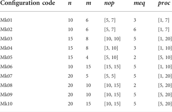
TABLE 4. Brandimarte’s benchmarks.

Since the proposed CEA-FJSP considers energy consummation of machine operation and coolant treatment in addition to makespan. Therefore, Brandimarte’s benchmarks are extended by adding seven additional parameters to generate CEA-FJSP scheduling instances. Table 5 lists the added parameters, where Unif denotes uniform distribution of real numbers and Rand denotes random selection. The processing time was measured in seconds instead of the unit time used in the original benchmarks to calculate the specific values of carbon emission. Carbon emission factors were set according to the Hong Kong SME Carbon Audit Toolkit (Liu et al., 2018). The Mki instances of Brandimarte’s benchmarks were changed to MkiEx instances after adding the additional parameters.

TABLE 5

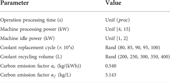
TABLE 5. Parameters added to extend Brandimarte’s benchmarks.

4.1.2 Evaluation metrics

Average makespan, $AC$, average total carbon emission, $AC$, and normalized performance, NP, were used to evaluate the performance of the proposed model. The smaller $AC$, $AT$ or $NP$ correspond to the better performance. These three metrics are defined as follows:

$\begin{array}{c}AC=\frac{1}{n}{\sum }_{i=1}^n{\left(C_{\max }\right)}_i\end{array}(19)$

$\begin{array}{c}AT=\frac{1}{n}{\sum }_{i=1}^n{TCE}_i\end{array}(20)$

$\begin{array}{c}NP=w_1\frac{AC-\underset{m_d\in \mathit{M}\mathit{S}}{\min }{AC}_d}{\underset{m_d\in \mathit{M}\mathit{S}}{\max }{AC}_d-\underset{m_d\in \mathit{M}\mathit{S}}{\min }{AC}_d}+w_2\frac{AT-\underset{m_d\in \mathit{M}\mathit{S}}{\min }{AT}_d}{\underset{m_d\in \mathit{M}\mathit{S}}{\max }{AT}_d-\underset{m_d\in \mathit{M}\mathit{S}}{\min }{AT}_d}\end{array}(21)$

where $n$ is the total number of testing instances, ${\left(C_{\max }\right)}_i$ and ${TCE}_i$ are the makespan and total carbon emission of the $i$ th instances. Method set, $\mathit{M}\mathit{S}$, is composed of the proposed mode and the scheduling methods used for comparison, and $d$ denotes the index of the scheduling method $m_d$. ${AC}_d$ and ${AT}_d$ denote $AC$ and $AT$ of $m_d$, respectively.

4.2 Training dynamics

Five Mk03Ex instances were generated in each training cycle based on the Mk03 configuration in Table 4 with the parameters in Table 5. These instances were used to train the proposed DRL scheduling model to produce the DRL-Mk03Ex scheduling solver. Table 6 lists the values of hyperparameters of Algorithm 1. Both weights $w_1$ and $w_2$ were set to 0.5 to equally evaluate the contribution of makespan and carbon emissions to the reward. Furthermore, reward scaling (Engstrom et al., 2020) was adopted to stabilize the training process. The hardware for training was a PC with a single Intel Xeon E5-2678 V3 @ 2.50 GHz CPU and a single NVIDIA RTX A2000 GPU. Algorithm 1 was implemented using Python 3.7, with PyTorch to deploy the network model.

TABLE 6

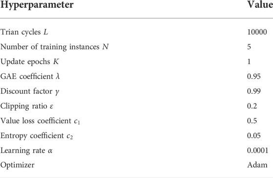
TABLE 6. Hyperparameter values of Algorithm 1.

Figure 4A–C show the training histories of the reward, $C_{\max }$ and $TCE$, respectively. It can be seen from Figure 4A that the reward gradually increases with the advance of the training process. Figure 4C shows that $TCE$ continuously contributes positively to the reward, as it decreases monotonously along the timeline. It can be seen from Figure 4B that $C_{\max }$ increases till about the 2200th cycle and then decreases until the end. The results show that the contribution of $TCE$ to the reward surpasses $C_{\max }$ in the early stage of optimization, and finally, both $TCE$ and $C_{\max }$ are optimized by the DRL scheduling model. All three curves in Figure 4 begin to converge around the 7000th cycle and all of them oscillate slightly thereafter. Therefore, the training process had better stop around the 7000th cycle or the performance could get worse, exhibiting a kind of overfitting behavior.

FIGURE 4

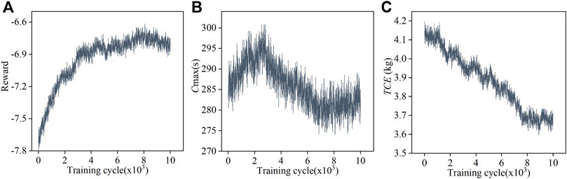
FIGURE 4. Training histories of (A) the reward, (B) the makespan, and (C) the total carbon emission.

4.3 Optimization ability

One hundred additional Mk03Ex instances different from those used in the training stage were generated to test the DRL-Mk03Ex against the proposed scheduling rules ${SR}_1$ to ${SR}_9$ and GA (Yin et al., 2017) respectively.

Figure 5 shows the performance of DRL-Mk03Ex over the Mk03Ex instances. It can be seen from the figure that DRL-Mk03Ex outperforms all the scheduling rules and GA on the testing instances, i.e., it achieves the lowest average makespan and the lowest average total carbon emission. Although GA and some scheduling rules (${SR}_5$, ${SR}_6$, ${SR}_8$) perform well in reducing makespan or total carbon emission, none of the scheduling rules and GA can simultaneously minimize the two objectives. Furthermore, DRL-Mk03Ex is also significantly better than the scheduling rules and GA in terms of $NP$. The results confirm the superiority and optimization ability of DRL-Mk03Ex.

FIGURE 5

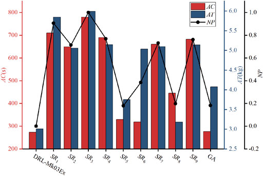
FIGURE 5. Performance of DRL-Mk03Ex over the Mk03Ex instances.

4.4 Generalization ability

The DRL scheduling solver built on the Mk03Ex instances (DRL-Mk03Ex) was tested on the Mk01Ex, Mk02Ex, and Mk04Ex to Mk10Ex instances. That is, to say, the instances used for testing were different from the ones used for training, and the difference was significant in the sense that the testing and the training instances were sampled from different configurations. To compare the performance, Table 7 shows the average results of three metrics over 100 instances for nine different instance configurations. The proposed scheduling rules ${SR}_1$ to ${SR}_9$ and GA are used as the baselines and the best values of each metric are highlighted in bold font in Table 7.

TABLE 7

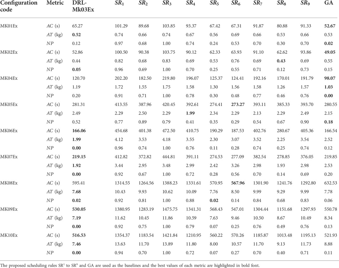
TABLE 7. Performance of DRL-Mk03Ex over the non-Mk03Ex instances.

Table 7 shows that DRL-Mk03Ex achieves the best solutions in most instances compared with the scheduling rules and GA. Furthermore, Mk01Ex and Mk02Ex instances have a simpler configuration than the Mk03Ex instances, while Mk04Ex to Mk10Ex instances have a more complex configuration. This means the DRL-Mk03Ex can be bidirectionally generalized. Besides, DRL-Mk03Ex can achieve comparable performance with GA in the simple scheduling instances, while surpassing GA in the complex instances. Moreover, DRL-Mk03Ex is also more robust than the scheduling rules. For example, $AC$ changes from 52.86 to 595.41 s for DRL-Mk03Ex, while from 100.5 to 1380.95 s for ${SR}_1$. The performance fluctuates even more wildly for the complex instances among the scheduling rules. For example, ${SR}_5$ and ${SR}_3$ achieve 560.22 and 1421.84 s as $AC$ values for the Mk10Ex instances, respectively.

4.5 Weight effect

The Mk03Ex instances were used to train the DRL scheduling model under various weight combinations $\left(w_1,w_2\right)$: ${WC}_1=\left(0.0,1.0\right)$, ${WC}_2=\left(0.25,0.75\right)$, ${WC}_3=\left(0.5,0.5\right)$, ${WC}_4=\left(0.75,0.25\right)$, and ${WC}_5=\left(1.0,0.0\right)$. Consequently, five DRL scheduling solvers were built. These solvers had the same model structure distinguished by different parameter values. Figure 6 illustrates the resultant $C_{\max }$ and $TCE$ as well as carbon emission components, ${CE}_p$, ${CE}_r$ and ${CE}_f$ for processing state, idle state, and coolant treatment, respectively, of the five solvers.

FIGURE 6

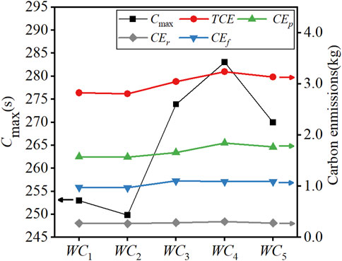
FIGURE 6. Effects of different weight combinations on makespan and carbon emission.

The results demonstrate the nonlinearity of the DRL scheduling solvers. The $C_{\max }$ does not vary monotonously with the weight $w_1$; nor does the carbon emission with the weight $w_2$, i.e., either the makespan or the carbon emission is affected jointly by $w_1$ and $w_2$. It also implies that the DRL scheduling solvers cannot directly control the sub-optimization objectives. Instead, the weights should be treated as optimization parameters in the sense that the weighted optimization objective can be figured out for a given instance by adjusting $w_1$ and $w_2$. For example, ${WC}_2$ is the best among the five weight combinations for the Mk03Ex instances.

For each weight combination, the three carbon emission components, ${CE}_p$, ${CE}_f$, and ${CE}_r$, contribute roughly 56%, 34%, and 10% to $TCE$, respectively. Specifically, the machines produce the most carbon emission when processing an operation, and the least carbon emission when in the idle state. The carbon emission caused by the coolant treatment is also nonnegligible. Furthermore, it can be observed that as ${CE}_p$, ${CE}_f$, and ${CE}_r$ maintain a similar tendency with the $TCE$ along the weight change. The results stimulate the possibility to simplify the representation of carbon emission by replacing $TCE$ with ${CE}_p$ or with the sum of ${CE}_p$ and ${CE}_f$.

5 Conclusion

In this study, a carbon emission-aware flexible job-shop scheduling problem denoted as CEA-FJSP is formulated and a DRL scheduling model is proposed to generate feasible scheduling solutions without extra searching. In the CEA-FJSP, the energy consumption of machine operation and the coolant treatment are identified as two main carbon emission sources. The proposed DRL scheduling model treats the CEA-FJSP as a Markov decision process where the scheduling agent interacts repeatedly with the scheduling environment, i.e., the temporary scheduling solution, to determine an appropriate action for a given state. The interaction is guided by the reward which represents the optimization objectives: minimizing makespan and carbon emission. The experimental results verify that the proposed DRL scheduling model achieves stronger optimization and generalization ability than the scheduling rules and GA, and the DRL scheduling model can be tuned by varying the weight combination. The future work should consider more carbon emission sources, more optimization objectives, and more flexible DRL framework to approach a more practical scheduling solution for the complex production scenarios.

Data availability statement

The original contributions presented in the study are included in the article/Supplementary Material, further inquiries can be directed to the corresponding author.

Author contributions

SW and JL were the principal authors for the text, and responsible for problem formulation, method design, experimental analysis, and manuscript writing. HT contributed to investigation. HT and JW contributed to the visualization together. All authors reviewed the final version of the manuscript and consented to publication.

Funding

This work was supported by the National Key R&D Program of China (Grant No. 2020YFB1708500), and the Science and Technology Planning Project of Guangzhou City (Grant No. 202102020882).

Conflict of interest

The authors declare that the research was conducted in the absence of any commercial or financial relationships that could be construed as a potential conflict of interest.

The handling editor UB declared a shared affiliation with the author HT at the time of review.

Publisher’s note

All claims expressed in this article are solely those of the authors and do not necessarily represent those of their affiliated organizations, or those of the publisher, the editors and the reviewers. Any product that may be evaluated in this article, or claim that may be made by its manufacturer, is not guaranteed or endorsed by the publisher.

References

Allahverdi, A., Ng, C. T., Cheng, T. E., and Kovalyov, M. Y. (2008). A survey of scheduling problems with setup times or costs. Eur. J. Oper. Res. 187 (3), 985–1032. doi:10.1016/j.ejor.2006.06.060

CrossRef Full Text | Google Scholar

Arulkumaran, K., Deisenroth, M. P., Brundage, M., and Bharath, A. A. (2017). Deep reinforcement learning: A brief survey. IEEE Signal Process. Mag. 34 (6), 26–38. doi:10.1109/MSP.2017.2743240

CrossRef Full Text | Google Scholar

Bhatti, U. A., Nizamani, M. M., and Mengxing, H. (2022a). Climate change threatens Pakistan’s snow leopards. Science 377 (6606), 585–586. doi:10.1126/science.add9065

PubMed Abstract | CrossRef Full Text | Google Scholar

Bhatti, U. A., Yan, Y., Zhou, M., Ali, S., Hussain, A., Qingsong, H., et al. (2021). Time series analysis and forecasting of air pollution particulate matter (PM 2.5): An SARIMA and factor analysis approach. IEEE Access 9, 41019–41031. doi:10.1109/ACCESS.2021.3060744

CrossRef Full Text | Google Scholar

Bhatti, U. A., Zeeshan, Z., Nizamani, M. M., Bazai, S., Yu, Z., and Yuan, L. (2022b). Assessing the change of ambient air quality patterns in Jiangsu Province of China pre-to post-COVID-19. Chemosphere 288, 132569. doi:10.1016/j.chemosphere.2021.132569

PubMed Abstract | CrossRef Full Text | Google Scholar

Brandimarte, P. (1993). Routing and scheduling in a flexible job shop by tabu search. Ann. Oper. Res. 41 (3), 157–183. doi:10.1007/BF02023073

CrossRef Full Text | Google Scholar

Brucker, P., and Schlie, R. (1990). Job-shop scheduling with multi-purpose machines. Computing 45 (4), 369–375. doi:10.1007/BF02238804

CrossRef Full Text | Google Scholar

Dai, M., Tang, D., Giret, A., and Salido, M. A. (2019). Multi-objective optimization for energy-efficient flexible job-shop scheduling problem with transportation constraints. Robot. Comput. Integr. Manuf. 59, 143–157. doi:10.1016/j.rcim.2019.04.006

CrossRef Full Text | Google Scholar

Du, Y., Li, J. Q., Chen, X. L., Duan, P. Y., and Pan, Q. K. (2022). Knowledge-based reinforcement learning and estimation of distribution algorithm for flexible job-shop scheduling problem. IEEE Trans. Emerg. Top. Comput. Intell. (Early Access), 1–15. doi:10.1109/TETCI.2022.3145706

CrossRef Full Text | Google Scholar

Engstrom, L., Ilyas, A., Santurkar, S., Tsipras, D., Janoos, F., Rudolph, L., et al. (2020). Implementation matters in deep policy gradients: A case study on PPO and trpo. arXiv [Preprint]. Available at: https://arxiv.org/abs/2005.12729.

Google Scholar

Feng, Y., Zhang, L., Yang, Z., Guo, Y., and Yang, D. (2021). “Flexible job-shop scheduling based on deep reinforcement learning,” in 2021 5th Asian Conference on Artificial Intelligence Technology (ACAIT), Haikou, China, 29-31 October 2021 (IEEE), 660–666. doi:10.1109/ACAIT53529.2021.9731322

CrossRef Full Text | Google Scholar

Fernandes, J. M., Homayouni, S. M., and Fontes, D. B. (2022). Energy-efficient scheduling in job shop manufacturing systems: A literature review. Sustainability 14 (10), 6264. doi:10.3390/su14106264

CrossRef Full Text | Google Scholar

Gao, K., Huang, Y., Sadollah, A., and Wang, L. (2020). A review of energy-efficient scheduling in intelligent production systems. Complex Intell. Syst. 6 (2), 237–249. doi:10.1007/s40747-019-00122-6

CrossRef Full Text | Google Scholar

Gutowski, T., Murphy, C., Allen, D., Bauer, D., Bras, B., Piwonka, T., et al. (2005). Environmentally benign manufacturing: Observations from Japan, europe and the United States. J. Clean. Prod. 13 (1), 1–17. doi:10.1016/j.jclepro.2003.10.004

CrossRef Full Text | Google Scholar

Han, B. -A., and Yang, J. -J. (2020). Research on adaptive job-shop scheduling problems based on dueling double DQN. IEEE Access 8, 186474–186495. doi:10.1109/ACCESS.2020.3029868

CrossRef Full Text | Google Scholar

Han, B. A., and Yang, J. J. (2021). A deep reinforcement learning based solution for flexible job-shop scheduling problem. Int. J. Simul. Model. 20 2, 375–386. doi:10.2507/IJSIMM20-2-CO7

CrossRef Full Text | Google Scholar

Lang, S., Behrendt, F., Lanzerath, N., Reggelin, T., and Müller, M. (2020). “Integration of deep reinforcement learning and discrete-event simulation for real-time scheduling of a flexible job shop production,” in 2020 Winter Simulation Conference (WSC), Orlando, FL, USA, 14-18 December 2020 (IEEE), 3057–3068. doi:10.1109/WSC48552.2020.9383997

CrossRef Full Text | Google Scholar

Lei, D., Zheng, Y., and Guo, X. (2017). A shuffled frog-leaping algorithm for flexible job-shop scheduling with the consideration of energy consumption. Int. J. Prod. Res. 55 (11), 3126–3140. doi:10.1080/00207543.2016.1262082

CrossRef Full Text | Google Scholar

Li, M., and Wang, G. G. (2022). A review of green shop scheduling problem. Inf. Sci. (N. Y). 589, 478–496. doi:10.1016/j.ins.2021.12.122

CrossRef Full Text | Google Scholar

Liu, C. -L., Chang, C. -C., and Tseng, C. -J. (2020). Actor-critic deep reinforcement learning for solving job-shop scheduling problems. IEEE Access 8, 71752–71762. doi:10.1109/ACCESS.2020.2987820

CrossRef Full Text | Google Scholar

Liu, Q., Tian, Y., Wang, C., Chekem, F. O., and Sutherland, J. W. (2018). Flexible job-shop scheduling for reduced manufacturing carbon footprint. J. Manuf. Sci. Eng. 140 (6), 061006. doi:10.1115/1.4037710

CrossRef Full Text | Google Scholar

Liu, R., Piplani, R., and Toro, C. (2022). Deep reinforcement learning for dynamic scheduling of a flexible job shop. Int. J. Prod. Res. 60 (13), 4049–4069. doi:10.1080/00207543.2022.2058432

CrossRef Full Text | Google Scholar

Luo, S. (2020). Dynamic scheduling for flexible job shop with new job insertions by deep reinforcement learning. Appl. Soft Comput. 91, 106208. doi:10.1016/j.asoc.2020.106208

CrossRef Full Text | Google Scholar

Luo, S., Zhang, L., and Fan, Y. (2021). Dynamic multi-objective scheduling for flexible job shop by deep reinforcement learning. Comput. Ind. Eng. 159, 107489. doi:10.1016/j.cie.2021.107489

CrossRef Full Text | Google Scholar

Luo, S., Zhang, L., and Fan, Y. (2019). Energy-efficient scheduling for multi-objective flexible job shops with variable processing speeds by grey wolf optimization. J. Clean. Prod. 234, 1365–1384. doi:10.1016/j.jclepro.2019.06.151

CrossRef Full Text | Google Scholar

Mokhtari, H., and Hasani, A. (2017). An energy-efficient multi-objective optimization for flexible job-shop scheduling problem. Comput. Chem. Eng. 104, 339–352. doi:10.1016/j.compchemeng.2017.05.004

CrossRef Full Text | Google Scholar

Monaci, M., Agasucci, V., and Grani, G. (2021). An actor-critic algorithm with deep double recurrent agents to solve the job-shop scheduling problem. arXiv [Preprint]. Available at: https://arxiv.org/abs/2110.09076.

Google Scholar

Naimi, R., Nouiri, M., and Cardin, O. (2021). A Q-Learning rescheduling approach to the flexible job shop problem combining energy and productivity objectives. Sustainability 13 (23), 13016. doi:10.3390/su132313016

CrossRef Full Text | Google Scholar

Ni, F., Hao, J., Lu, J., Tong, X., Yuan, M., Duan, J., et al. (2021). “A multi-graph attributed reinforcement learning based optimization algorithm for large-scale hybrid flow shop scheduling problem,” in Proceedings of the 27th ACM SIGKDD Conference on Knowledge Discovery and Data Mining (KDD), Singapore, Aug 14, 2021 - Aug 18, 2021, 3441–3451. doi:10.1109/ICCECE54139.2022.9712705

CrossRef Full Text | Google Scholar

Pan, Z., Wang, L., Wang, J., and Lu, J. (2021). Deep reinforcement learning based optimization algorithm for permutation flow-shop scheduling. IEEE Trans. Emerg. Top. Comput. Intell. (Early Access), 1–12. doi:10.1109/TETCI.2021.3098354

CrossRef Full Text | Google Scholar

Park, J., Chun, J., Kim, S. H., Kim, Y., and Park, J. (2021). Learning to schedule job-shop problems: Representation and policy learning using graph neural network and reinforcement learning. Int. J. Prod. Res. 59 (11), 3360–3377. doi:10.1080/00207543.2020.1870013

CrossRef Full Text | Google Scholar

Qu, S., Wang, J., and Shivani, G. (2016). “Learning adaptive dispatching rules for a manufacturing process system by using reinforcement learning approach,” in 2016 IEEE 21st International Conference on Emerging Technologies and Factory Automation (ETFA), Berlin, Germany, 06-09 September 2016 (IEEE). doi:10.1109/ETFA.2016.7733712

CrossRef Full Text | Google Scholar

Ren, J. F., Ye, C. M., and Yang, F. (2020). A novel solution to JSPS based on long short-term memory and policy gradient algorithm. Int. J. Simul. Model. 19 (1), 157–168. doi:10.2507/IJSIMM19-1-CO4

CrossRef Full Text | Google Scholar

van Ekeris, T., Meyes, R., and Meisen, T. (2021). “Discovering heuristics and metaheuristics for job-shop scheduling from scratch via deep reinforcement learning,” in Proceedings of the Conference on Production Systems and Logistics (CPSL), Online, 10-11 August 2021, 709–718. doi:10.15488/11231

CrossRef Full Text | Google Scholar

Wu, X., and Sun, Y. (2018). A green scheduling algorithm for flexible job shop with energy-saving measures. J. Clean. Prod. 172, 3249–3264. doi:10.1016/j.jclepro.2017.10.342

CrossRef Full Text | Google Scholar

Xu, B., Mei, Y., Wang, Y., Ji, Z., and Zhang, M. (2021). Genetic programming with delayed routing for multiobjective dynamic flexible job-shop scheduling. Evol. Comput. 29 (1), 75–105. doi:10.1162/evco_a_00273

PubMed Abstract | CrossRef Full Text | Google Scholar

Yan, Q., Wu, W., and Wang, H. (2022). Deep reinforcement learning for distributed flow shop scheduling with flexible maintenance. Machines 10 (3), 210. doi:10.3390/machines10030210

CrossRef Full Text | Google Scholar

Yin, L., Li, X., Gao, L., Lu, C., and Zhang, Z. (2017). A novel mathematical model and multi-objective method for the low-carbon flexible job shop scheduling problem. Sustain. Comput. Inf. Syst. 13, 15–30. doi:10.1016/j.suscom.2016.11.002

CrossRef Full Text | Google Scholar

Zeng, Y., Liao, Z., Dai, Y., Wang, R., and Yuan, B. (2022). Hybrid intelligence for dynamic job-shop scheduling with deep reinforcement learning and attention mechanism. arXiv [Preprint]. Available at: https://arxiv.org/abs/2201.00548.

Google Scholar

Zhang, C., Song, W., Cao, Z., Zhang, J., Tan, P. S., and Xu, C. (2020). Learning to dispatch for job-shop scheduling via deep reinforcement learning. arXiv [Preprint]. Available at: https://arxiv.org/abs/2010.12367.

Google Scholar

Zhang, H., Xu, G., Pan, R., and Ge, H. (2022). A novel heuristic method for the energy-efficient flexible job-shop scheduling problem with sequence-dependent set-up and transportation time. Eng. Optim. 54 (10), 1646–1667. doi:10.1080/0305215X.2021.1949007

CrossRef Full Text | Google Scholar

Zhang, J., Ding, G., Zou, Y., Qin, S., and Fu, J. (2019). Review of job shop scheduling research and its new perspectives under Industry 4.0. J. Intell. Manuf. 30 (4), 1809–1830. doi:10.1007/s10845-017-1350-2

CrossRef Full Text | Google Scholar

Zhao, Y., Wang, Y., Tan, Y., Zhang, J., and Yu, H. (2021). Dynamic jobshop scheduling algorithm based on deep q network. IEEE Access 9, 122995–123011. doi:10.1109/ACCESS.2021.3110242

CrossRef Full Text | Google Scholar