 Yu Yang
 Qing He1*
 Liu Yang
94% of researchers rate our articles as excellent or good
Learn more about the work of our research integrity team to safeguard the quality of each article we publish.
Find out more
METHODS article
Front. Environ. Sci., 28 November 2022
Sec. Environmental Informatics and Remote Sensing
Volume 10 - 2022 | https://doi.org/10.3389/fenvs.2022.1055807
This article is part of the Research TopicTowards Sustainable Urban Development: Use of Geographic Big Data for Spatial PlanningView all 25 articles
Real-time monitoring of urban high-altitude data is an important goal in the construction and development of smart cities today. However, with the development of modern cities, the monitoring space becomes complicated and narrow because of the different building heights and no-fly zones, which makes UAV trajectory planning more difficult. In this paper, a multi-strategy sparrow search algorithm (MSSA) is proposed to solve the UAV trajectory planning problem in a three-dimensional environment. The algorithm aims to minimize the flight distance and maximize the use efficiency of the UAV. First, the improved algorithm employed a reverse-learning strategy based on the law of refraction to improve the search range and enhance the optimization performance. Second, we introduced a random step size generated by Levy flight into the position update strategy of the participant. The algorithm accuracy and speed of convergence were improved by the randomness feature. Finally, the algorithm incorporated the Cauchy mutation to improve the scout position, which enhanced its ability to jump out of the local optimum of the algorithm. Sixteen benchmark test functions, Wilcoxon rank sum test, and 30 CEC2014 test function optimization results demonstrated that MSSA had better optimization accuracy, convergence speed, and robustness than the comparison algorithms. In addition, the proposed algorithm was applied to the UAV trajectory planning problem in different complex 3D environments. The results confirmed that the MSSA outperformed the other algorithms in complex 3D trajectory planning problems.
With the continuous development of information technology and smart cities (Van Steen and Leiba, 2018), UAV technology plays an important role in urban emergencies and transportation networks. Due to their usefulness, reliability, safety, and relatively low cost (Rodríguez et al., 2021), UAVs (commonly referred to as drones) have become an indispensable part of the operations of a smart city. In research on UAV technology, trajectory planning is the key to the whole system. The main technical difficulty is to find a feasible way to avoid obstacles when the starting and ending points are known (Zhao et al., 2018). At present, many cities around the world are facing the problem of traffic congestion. In particular, there are periodic or sudden increases in the number of vehicles during peak hours, large events, construction work or accidents. In an emergency, the use of drones can assist traffic police in implementing security in smart cities, and rapid deployment can collect real-time information (Qadir, 2021). However, due to the complexity of the flight environment in modern urban spaces, UAV monitoring tasks are becoming more and more difficult (Mohamed, 2020). Therefore, how to outfit a UAV so that it can find a flight path that avoids obstacles but still maintains the shortest distance to the destination is a main focus of today’s UAV research.
The process of UAV trajectory planning is a combinatorial optimization problem. Currently, UAVs have a low efficiency in completing tasks in complex areas because of the large scale of the mathematical model and its high computational complexity. The complexity and difficulty of real-world optimization problems continue to increase, as they are subject to strong constraints and require long computation times, non-convexity, and wide search space (Shin and Bang, 2020). Path length is the primary factor to be considered in engineering scenarios, and optimizing path is of great research significance for improving flight efficiency. Path optimization aims to maximize the execution efficiency of the UAV within permissible limits. The methods for deducing the optimal power flow in trajectory planning can be divided into traditional optimization algorithms and metaheuristic algorithms. Traditional optimization algorithms mainly include the gradient descent method Salgado et al., 1990), the Newton method (Tinney ea al., 1967), linear programming (Olofsson et al., 1995), and the interior point method (Momoh, 1999). These algorithms are characterized by their use of the objective function to solve the first- or second-order gradient of control variables. Traditional optimization algorithms are generally trapped in local optima; hence, the optimization results depend greatly on the initial value in solving large-scale problems. In recent years, researchers have proposed many metaheuristic algorithms by simulating various biological behaviors and physical phenomena in nature. The metaheuristic algorithms commonly include Archimedes optimization algorithm (AOA) (Hashim ea al., 2021), the tunicate swarm algorithm (TSA) (Kaur et al., 2020), Aquila optimization (AO) (Abualigah et al., 2021), Harris hawks optimization(HHO) (Heidari et al., 2019), ant colony optimization (ACO) (Zhang et al., 2015), grey wolf optimizer (GWO) (Mirjalili et al., 2014), differential evolution (DE) (Price, 2013), and particle swarm optimization (PSO) (Marini and Walczak, 2015).
Metaheuristic algorithms are widely used to solve problems related to power system optimization because of their simple structure, few adjustment parameters, and lack of need for gradient information. Wen et al. (2022) proposed a novel heuristic algorithm based on a three-dimensional (3D) UAV deployment scheme that could be used by a number of covered users without increasing the number of UAVs. Fan et al. (2022b) proposed an improved RRT algorithm based on the process of extending the random tree, and introduced ACO to make the planning path asymptotically optimal. Jia et al. (2022) described a UAV path coverage algorithm based on a ‘greedy’ strategy and ACO (Zhang et al., 2015) to minimize flight time and maximize coverage. Shin and Bang (2022) offered an improved PSO algorithm for path optimization. Belge et al. (2022) developed a new UAV trajectory planning algorithm for optimal path planning and tracking using HHO and GWO. Zhang et al. (2021) proposed an adaptive convergence factor adjustment strategy and an adaptive weight factor to update the individual’s position based on GWO. Zhang et al. (2015) created an improved constrained DE algorithm to generate an optimal feasible route. Chang et al. (2021) introduced Q-learning to improve the dynamic window algorithm and increase its success rate for path planning in an unknown mountainous environment. However, the calculations necessary to use this algorithm are more complex, and beyond the low computational power of the UAV; the local path planning strategy is not applicable to global optimization.
The sparrow search algorithm (SSA), a swarm intelligence optimization algorithm proposed by Xue and Shen (2020), combines simplicity with flexibility. It is very effective for solving highly nonlinear, multi-variate, and multimodal function optimization problems. Many researchers have studied the SSA algorithm and confirmed that it outperforms the GWO, PSO (Poli et al., 2007), and GA (Whitley, 1994) in solving numerous types of optimization problems. The SSA has been used in many other fields. Wu et al. (2021) reported the application of GGSC-SSA to solve the traveling salesman problem (TSP); Fan et al. (2022a) even utilized SSA to improve the quality of medical images; but few published reports exist on the application of SSA to UAV trajectory planning. Here we propose a new metaheuristic optimization algorithm based on the SSA and referred to as MSSA. Since the B-spline curve cannot guarantee absolute accuracy of the interpolation points (Thompson and Patel, 1987), we used the cubic spline interpolation method to smooth the path. First, we established a 3D environmental model for UAV trajectory planning that included reference terrain, obstacle areas, and threat areas. Second, a comprehensive cost evaluation model of UAV flight was proposed as the objective function. The path was smoothed by the method of cubic spline interpolation to obtain an optimal trajectory. Lastly, we analyzed the results and verified the effectiveness and feasibility of the proposed algorithm in planning the UAV’s trajectory in the 3D model.
With the leapfrog development of information science, various new technologies employing AI for advanced communication and control have been put forward, many of which have been applied in UAV operating systems, providing a foundation for the rapid deployment of UAVs for numerous uses. At present, UAVs have become an important accessory for air power in the military, which can perform battlefield reconnaissance, supply delivery missions, and enemy target strikes. In addition to military applications, civilian applications of UAVs have also been accelerating in a number of areas, including traffic supervision, disaster relief, inspections, and scientific data gathering. The UAV trajectory problem is a multi-constraint combinatorial optimization problem. Due to the size of the mathematical model and the complexity of the calculation, a suitable cost function and an effective trajectory planning method are both crucial to the efficient implementation of UAVs.
Finding an optimal path using planning algorithms is the main goal of UAV trajectory planning, and this path must meet performance indicators and overcome limitations. The UAV may encounter several hurdles throughout this trajectory planning process, including terrain threats, fire, no-fly zones, and performance limitations imposed by the equipment itself (Bagherian and Alos, 2015). For testing of this algorithm, we held the UAV’s speed constant and kept track of the distribution of the mission environment’s peaks and no-fly zones to make the computation model simpler. The challenge of trajectory planning was changed into a static space routing mission problem. The trajectory planning system is depicted in Figure 1. Figure 1 illustrates the components of the UAV trajectory planning process, which included environmental modelling, cost function definition, track optimization, and track smoothing. Our goal in this study was to establish an optimal flight path before the UAV flight mission. By sending the algorithm’s best path data to the UAV’s flight master control system, the flight trajectory planning will be accomplished successfully.
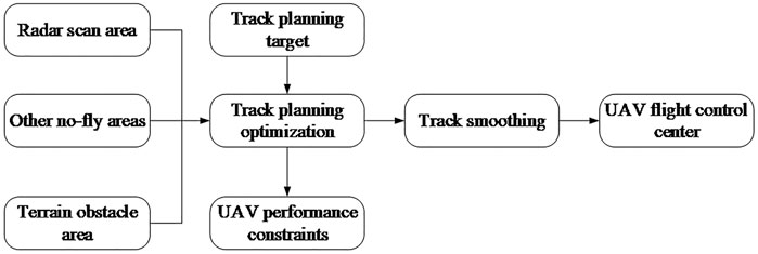
FIGURE 1. Flow chart of the trajectory planning system.
According to the 3D space environment there were significant changes in altitude and terrain complexity along the route (Dübel and Schumann, 2017), and the flight path may be categorized into areas of plains, mountainous regions, and hilly areas. A large number of complex factors need to be considered if the flight must pass through a mountainous or hilly area. The UAV needs to adjust the travel direction and the flight altitude continuously in those complex environments, and trajectory planning must be carried out in 3D space. In this study, we developed two distinct settings for UAV trajectory planning and used a function simulation approach to characterize landform properties. Eq. 1 displays the function expression:
where (x, y) is the point coordinate of the terrain projected onto the horizontal plane and z is the height of the corresponding point coordinate on the Z axis. In Eq. 1, a, b, c, d, e, f, g, and h are constant coefficients, and the different topography features can be obtained by changing the size of the constant coefficients in the modelling process. In this test flight, we simulated the geographical environment, such as mountains and hills, by superimposing the mountain model on the base terrain. The mathematical expression of the topography model is shown in Eq. 2:
In Eq. 2, ho and hi represent the height of the reference terrain and the ith peak, respectively, (xoi, yoi) represent the central coordinate position of the ith peak, and ai and bi are the slopes of the ith mountain along the X and Y axes, respectively. The peaks can show different length and width characteristics by adjusting the value of those parameters. We can obtain Eq. 3 from Eqs 1, 2:
In practical situations, UAVs frequently encounter areas with tall buildings and trees that threaten flight safety, or no-fly areas where UAVs have to avoid obstacles. Therefore, we included a certain number of threat areas in the UAV trajectory plan to judge the obstacle avoidance performance of the algorithm. Graphically, we represented a danger area as a cylinder with a radius of R to simplify the model. The center position of each cylinder affords the greatest threat to the UAV, and the threat decreases from the center to the outside.
When completing challenging jobs, the UAV trajectory planner must take into consideration the inherent performance restrictions of the drone based on environmental modeling. The final results produced by the algorithm can be made to comply with the specifications and guarantee that the intended flight route is valid with a suitable design of the trajectory evaluation function. We devised a sophisticated track evaluation algorithm to plan the UAV trajectory based on real circumstances. The indicators that most affected the performance of the UAV included track length, flight height, minimum step size, corner cost, and maximum climb angle.
Trajectory planning is inseparable from searching for the shortest path because the length of the track is very important for successful trajectory planning. Obviously, the shortest route can save on fuel and time and reduce the chance occurrence of unknown threats. We defined the path as the value of the distance from the starting to the ending point. Suppose a complete route has n nodes, the distance between the ith and the i+1-th waypoint is expressed as li, the coordinates of these two flight points are expressed as (xi, yi, zi) and (xi+1, yi+1, zi+1), denoted the two points as g(i) and g(i+1), respectively. The trajectory needs to satisfy the following conditions in Eq. 4:
The UAV will run the risk of crashing or being shot down if it is unable to avoid obstacles or flying into a hazard region, which is indicated by the Lpath being Lpath = ∞. Because infinite functions are challenging to depict in real-world situations, we deal with them in a penalizing approach. The UAV should fly as low as it can in the real world to avoid potential radar detection. However, it is crucial to choose a steady flight altitude because a low flight altitude would increase the probability of the UAV colliding with trees, mountains, or the ground. The flying altitude should not change much because a constant altitude eases the strain on the control system and conserves fuel. To make the UAV flight safer, the flight height model given in Eq. 5:
The maneuverability of a UAV is limited by its corner cost function. During the flight of the UAV trajectory planning, the turning angle should not be greater than the preset maximum turning angle, because of the turning angle size will affect the flight stability. In this paper, we set the maximum turning angle to
In Eq. 6, |a| represents the length of the vector a. Through the description of the above three aspects, we established the cost function of UAV trajectory planning as follows in Eq. 7:
Jcost is the total cost function, and in the parameters wi, i = 1, 2, 3 represent the weight of each cost function and satisfy the conditions of Eq. 8:
We obtained a track consisting of line segments by processing the total cost function effectively. However, the resulting track is only theoretically feasible, it is necessary to smooth the track to meet the actual situation. In this paper, cubic spline interpolation is used to smooth the UAV trajectory because the B-spline curve cannot guarantee the absolute accuracy of the interpolation points.
The sparrow search algorithm is a new type of swarm intelligence optimization algorithm inspired by the feeding behavior of sparrows in nature. During the food search process, the sparrow population is divided into two roles: discoverer and follower. Discoverers generally make up 10%–20% of the population and lead the other individuals in the search for food. The discoverers have a high fitness and ability to expand the search range, while the remaining sparrows follow the discoverers to the destination. The population requires a particular number of sparrows to work as scouts and issue warnings to remind the populace that they can take action in time when the adversaries attack to escape the threat of natural enemies. The location update formula for the discoverer is as follows in Eq. 9:
In Eq. 9, h represents the current number of iterations and T is the maximum number of iterations. The value of xi,j denotes the current position of the ith sparrow in the jth dimension. The term, α, is a random number between 0 and 1, and Q is a random value obeying a standard normal distribution. L represents a 1×D matrix with all elements 1, alarm value R2∈[0,1], and safety value ST∈[0.5,1].
When R2<ST, it indicates that the surrounding environment is currently in a safe state, and the discoverers can search for food on a wide scale. If R2>ST, it means that there may be natural enemies in the surrounding environment, and the discoverers will quickly lead the population from the current position to avoid predators. Followers update their position according to their fitness ranking, and the positional update is described in Eq. 10:
In Eq. 10, xt w and xt+1 p represent the global worst position of the population at the tth iteration and the global optimal position of the population at the t+1-th iteration, respectively. A is a matrix of 1×D in which an element is only -1 or +1, with A+ = AT(AAT)−1. When i > n/2, it indicates that the ith participant is in a hungry state with poor fitness. In order to obtain higher energy, the participant needed to fly farther to find food. If i < n/2, the ith follower will find a random location near the current optimal position xp to forage. The location of the scouter has been updated as shown in Eq. 11:
where K is a step coefficient, which is a random number in [-1, 1], and K represents the moving direction of the sparrows. Q is a value close to infinitesimal, which exists to avoid the denominator being zero. fi represents the fitness values of the ith sparrows, fg and fw are the global optimal fitness and global worst fitness values within the current search scope, respectively, ε is the smallest real number, preventing the occurrence of 0 in the denominator. Individual sparrows face danger at the edge and approach the globally optimal sparrow when fi ≠ fg. The individual sparrows in the center of the group can randomly walk among other individuals when fi = fg. This setup aims to avoid too many individuals reaching a local optimum, where the algorithm stops iterating and falls into a local optimum.
The original SSA algorithm used a simple random function to generate the initial population, which cannot guarantee the diversity of the population and the stability of the algorithm. In the sparrow population, the foraging ability of the discoverers determines the foraging direction and foraging area of the population and also indicates the quality of the solution found by the algorithm. The formula for updating the discoverers’ positions is one of the key formulas in the SSA. In the later iterations of the SSA, the sparrow population gradually approaches to the optimal individual, which leads to a lack of population diversity and a tendency toward premature convergence of the algorithm. In the SSA, it can be seen from Eq. 9 that each dimension of the individual discoverer decreases when R2<ST. This leads to a decrease in the population diversity of the algorithm in its later iterations and a lack of convergence accuracy. In the iterative process of the algorithm, the location update of sparrows mainly depends on the information exchanged among individuals, which easily produces population aggregation and leads to a lack of diversity. Then, according to Eq. 10, a large number of followers will flood into the search area around the finder. When they perceive that the finder has searched for a better food location, the high population density around the finder educes the diversity of population positions and easily falls into a local optimum. In summary, we propose three corresponding improvement strategies for the original SSA algorithm, which is prone to local optimal values and insufficient convergence accuracy. The specific strategies are discussed below.
For the SSA in the finder stage, with the continuous expansion of the search range, a broad and flexible search mechanism is the key to guiding the entire sparrow population to find food and avoid danger. When R2 < ST, the discoverer individuals of each dimension decrease. To better realize the leading role of the discoverer, this paper proposes a reverse learning strategy based on the law of refraction. We calculate the reverse solution of the candidate solution and select the better solution to continue the iterative calculation to effectively enhance the diversity of the algorithm and help the algorithm jump out of the local extreme value space.
As shown in Figure 2, O is the center point of [a, b], x∈[a, b]; the global optimal individual X takes O as the center point to find its corresponding reverse individual X′, where a represents the upper bound and b represents the lower bound. It can be derived from the law of refraction shown in Eq. 12:
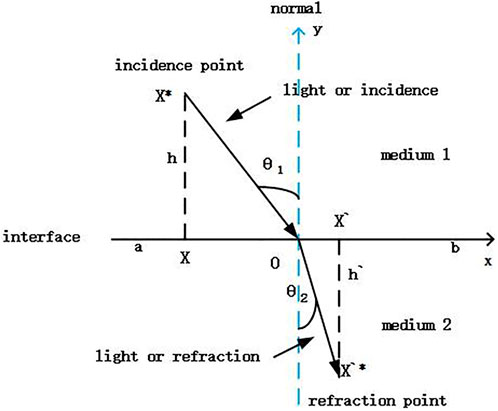
FIGURE 2. Refraction-learning process in one-dimensional space.
Assuming the scaling factor
Extend Eq. 13 to n-dimensional space to obtain:
In this formula, aj and bj represent the jth dimensional vector of the upper bound and the jth dimensional vector of the lower bound, respectively; xj and x' j represent the jth dimensional vector of X and x’, respectively. Refraction reverse learning is performed on the optimal solution in the population, and each dimension value is mapped to the solution space to obtain a reverse solution, which not only avoids the interference between various dimensions but also expands the search range of the algorithm.
Although the reverse learning strategy of the refraction law can help the algorithm to jump out of the local optimal value and improve the solution accuracy of the algorithm, it cannot expand the search range of the original population in the optimization process. Therefore, we introduced the Levy flight strategy to expand the follower’s optimal range.
According to Eq. 10, a large number of followers in SSA will flood into the search area around the discoverers when they perceive that the finder has searched for a better food location, which has obvious convergence and makes the population density of the search area too high around the discoverers. This situation will reduce the diversity of population positions and easily fall into a local optimum. In this paper, the random step size s generated by Levy’s flight is introduced into the follower’s location update strategy, and the uncertainty of Levy’s flight direction and step size is used to enhance the multiplicity of follower’s search direction, thus improving the diversity of population locations and avoiding the search from falling into local optimal value. The random step size s of the Levy flight can be calculated by Eq. 15, and the result is shown in Figure 3:
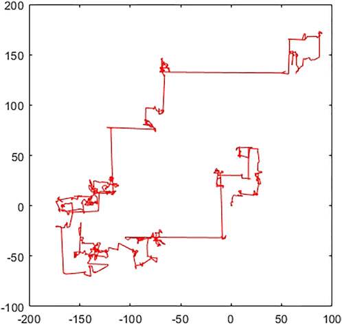
FIGURE 3. Step size of 100 Levy flights.
Figure 3 shows that Levy flight shuttles each other due to short and long distance searches, producing random steps s with no definite direction or size. By introducing the Levy flight strategy, followers can both roughly search over a large range and finely search over a small range as they approach the discoverer, which can effectively avoid convergence and enhance the diversity of population locations. The formula for updating the position of the follower was changed from Eqs 10–16 with the addition of the Levy flight strategy:
According to Formula 10, it can be seen that the individual with lower fitness value as a follower will reset the solution to a number near 1 after updating according to the formula, which is more effective for some objective functions whose optimal convergence solution is near 1 or 0. However, in practical engineering applications, the sparrows generally fly to places with lower fitness values on the whole. At the same time, the sparrow individuals with moderate fitness values are directly replaced by the current best individual. Although the convergence speed is improved to a certain extent, it will waste the search area of this part of the sparrow population and reduce the search accuracy. Comprehensively comparing the characteristics of the individual fitness values of followers, sparrows with moderate fitness values search in the direction of the best sparrow individual according to the current search area, while sparrow individuals with low fitness value fly to search near the best position of the finder. The positions updated by Levy flight of the follower is changed from Eqs 16, 17:
In the SSA, the scouters enhance the global exploration ability of the algorithm to some extent, and the ability to jump out of the local optimal value is stronger if the number of scouters is a high percentage of the whole sparrow population. However, the random selection of scouters limits the more active sparrow individuals. The mechanism of fixing the number of scouter in the sparrow optimization algorithm slows down the optimization accuracy and convergence speed to a certain extent. Therefore, the improved scouter formula proposed in this paper on the original Eq. 11 is as follows:
Because the sparrow optimization algorithm easily falls into a local optimum, the peak value of the Cauchy distribution function at the origin is small, but the distribution at both ends is relatively long. Because the range of the Cauchy distribution function is relatively wide, it is easier to jump out of the local optimum by using the distribution at both ends of the Cauchy variation (Li et al., 2017). We used the Cauchy mutation to generate larger disturbances near the currently mutated sparrow individual to improve the local search ability of the algorithm and expand the search space of the algorithm. The standard Cauchy distribution function formula is as follows:
If the random variable x of the Cauchy distribution obeys the position parameter of x0 and the scale parameter of
There are two main differences because the density function of the Cauchy distribution is similar to the Gaussian density function. On the one hand, the Cauchy distribution in the vertical direction is slightly smaller than the Gaussian distribution. On the other hand, the closer the Cauchy distribution is to the horizontal axis in the horizontal direction, the slower the change, so the Cauchy distribution can be regarded as infinite.
The comparison of the two distributions is shown in Figure 4. The Cauchy distribution and the Gaussian distribution have certain similarities and their own characteristics. The Cauchy distribution has a wider range than the Gaussian distribution. The Cauchy distribution easily generates a random number far from the origin, which means that the sparrow individual after Cauchy mutation has a higher probability of jumping out of the local optimal area. In addition, the peak value of the Cauchy distribution function is lower than that of the Gaussian distribution, which can shorten the search time of the mutated sparrow individuals around the neighborhood. Therefore, this paper integrates the Cauchy mutation to improve the scouter position update strategy, increases the diversity of the population and improves the ability of the algorithm to jump out of the local optimum. The position update formula is as follows:
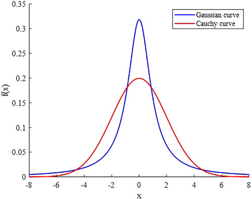
FIGURE 4. Gaussian curve and Cauchy curve distribution diagram.
Eqs 9–11, derived from the original work of SSA, specify how the sparrow is updated and construct the basic flow of the algorithm. Based on the idealization and feasibility of the above model, the basic steps of the improved SSA can be summarized in the pseudo-code shown in Algorithm 1.
The computer configuration used in the simulation experiment is Intel Core i7-6700HQ, the main frequency is 2.60 GHz, 8 GB memory, 64 bit operating system, and the computing environment is MATLAB 2019(b). We compare the SSA, GWO, WOA (Mirjalili and Lewis, 2016), TSA, and EO (Faramarzi et al., 2020) with MSSA. The basic parameters of the algorithms were set to the same value, including population size N = 30, the maximum number of iterations Tmax = 500. The test function dimensions were divided into low-dimensional (d = 30) and high-dimensional (d = 200 and d = 500).
To test the optimization performance of the MSSA algorithm, 16 benchmark functions with different characteristics used in the literature were selected for the function optimization test. The selected test functions were divided into three categories. The first category was the single-modal test function, f1-f6, which is mainly used to evaluate the optimization accuracy and convergence speed of the algorithm. The second type is the multi-modal test function, f7-f11, which is used to test the exploration ability of the algorithm and the ability to jump out of the local optimal value. The third type is the fixed multi-modal test function, f12-f16. This paper used the 16 benchmark functions to evaluate the comprehensive ability of the algorithm. The detailed description and related information are shown in Table 1.
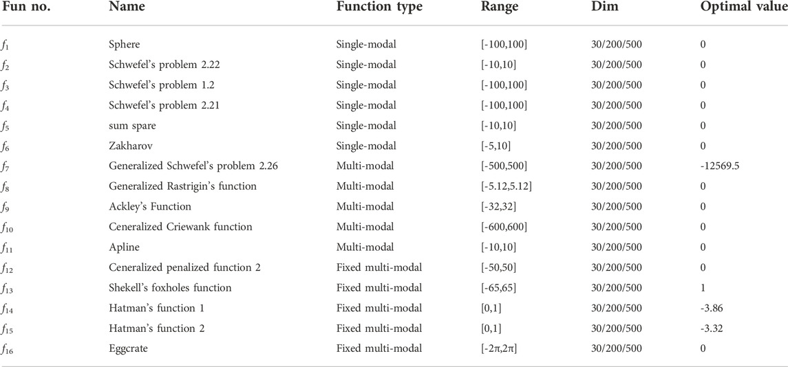
TABLE 1. Introduction to benchmark functions.
To fully verify the optimization effect of the proposed improved strategy, we denoted the three improvement strategies as SSA1, SSA2, and SSA3, and compare them with SSA and MSSA. Each algorithm was independently run 30 times on 16 benchmark functions, and the optimal value, worst value, mean value, and standard value were recorded. The optimal value and the worst value reflected the single optimization ability of the algorithm, the average value reflected the convergence accuracy, and the standard deviation reflected the stability and robustness of the algorithm. Parameters were uniformly set as follows: population size N = 30, search space dimension dim = 30, and maximum number of iterations, Tmax = 500. The results of experimental optimization are shown in Table 2:
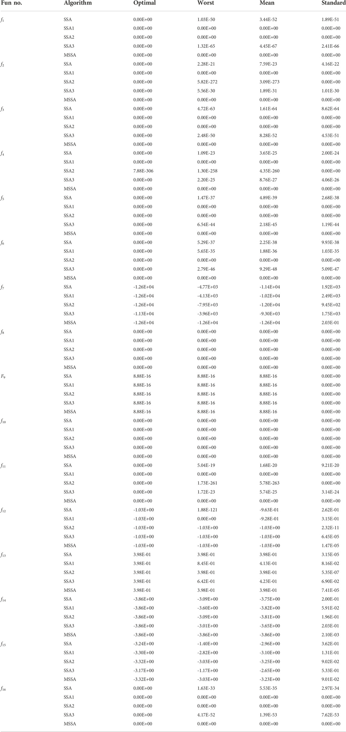
TABLE 2. Comparison of optimization results of different improvement strategies for SSA.
Table 2 shows that for the single-modal test functions, f1-f6, MSSA can find the theoretical optimal value, illustrating that the stability is strong. At the same time, SSA1 can reach the theoretical optimal value and the more stable standard, showing that the introduction of the lens imaging learning strategy helps the algorithm to jump out of the local optimal value. SSA2 can reach the optimal theoretical value in f1, f2, f5, and f6, indicating that adding Levy flight can help the population to deeply mine the global optimal values and improve the global search ability of the algorithm. For the multi-modal test functions, f7-f11, there are a large number of local extremes distributed in their solution space, and it is difficult for the algorithm to perform global optimization. The MSSA and other comparative algorithms fall into local optimal solutions when solving function f9. But MSSA has higher convergence accuracy and stability in other test functions, and the standards are more stable than other algorithms.
For the fixed multi-modal functions, f12-f16, MSSA can find the theoretical optimal value, and the stability is extremely strong and the standard value is lower than SSA1, SSA2, and SSA3, indicating that MSSA has stronger stability and robustness.
We used the average convergence curve to reflect the dynamic convergence characteristics of the MSSA in this paper. We make the algorithm run 30 times independently under the population size N = 30, maximum number of iterations Tmax = 500, and the search dimension dim = 30. Figure 5 presents the average convergence curves of the 16 benchmark functions.
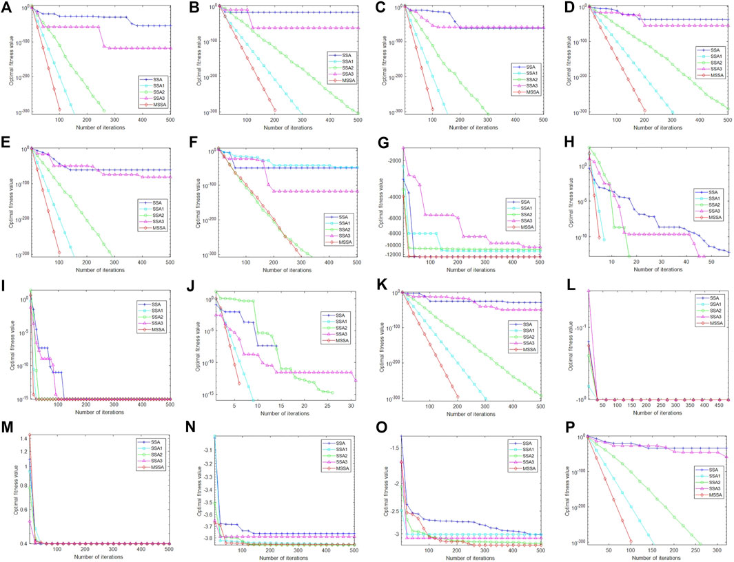
FIGURE 5. Mean convergence curve of the benchmark function. (A) f1 mean convergence curve. (B) f2 mean convergence curve. (C) f3 mean convergence curve. (D) f4 mean convergence curve. (E) f5 mean convergence curve. (F) f6 mean convergence curve. (G) f7 mean convergence curve. (H) f8 mean convergence curve. (I) f9 mean convergence curve. (J) f10 mean convergence curve. (K) f11 mean convergence curve. (L) f12 mean convergence curve. (M) f13 mean convergence curve. (N) f14 mean convergence curve. (O) f15 mean convergence curve. (P) f16 mean convergence curve.
Figure 5 shows that the MSSA has a higher optimization accuracy solution rate and faster convergence speed in f1-f5 than under the same number of iterations. The values of f7-f11 and f16 show that the MSSA is able to guarantee the exploration ability and illustrate that the MSSA can ensure the development ability without losing the population diversity and optimization stability. For f6 and f12-f14, the MSSA can converge to the optimal value faster in the later stages, which indicates that adopting the three strategies can help the algorithm jump out of the local optimal value effectively. In general, the MSSA average convergence curve is below the four comparison algorithms and takes fewer iterations to reach the theoretical optimal. From Table 2 and Figure 5, the result illustrates that the MSSA has higher convergence accuracy, convergence speed, stronger stability, and better robustness. The experimental results verify the effectiveness of the proposed algorithm and achieve the purpose of improving the standard SSA.
To further test the optimization characteristics of the MSSA algorithm for the benchmark function, this paper chose the standard SSA, GWO, WOA, TSA, EO, and MSSA to compare for optimization performance. For each benchmark function, the search dimension is set to dim = 30/200/500, the maximum number of iterations Tmax = 500 and the population size is N = 30. The test functions of Table 1 are used to perform the optimization comparison test, and each algorithm is run 30 times independently. The comparison results are shown in Table 3:
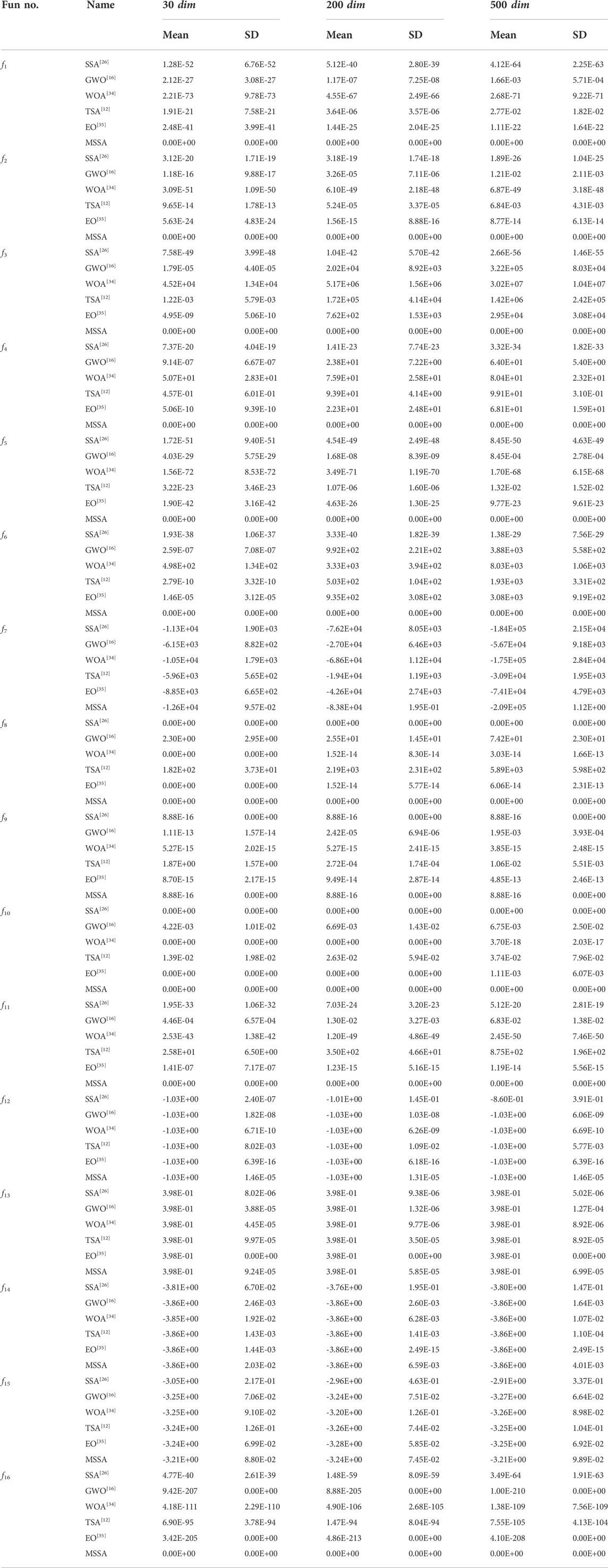
TABLE 3. Comparison with the results of five metaheuristic algorithms.
As seen from Table 3, the solution rate of MSSA can reach 100% when solving for the single-modal test function, f1-f6, which indicates that MSSA has good optimization accuracy and robustness. For the multi-modal test function, f7-f11, MSSA can find the theoretical optimal value. For the fixed multi-modal test function, f12-f16, the MSSA solution results are very close to or equal to the theoretical optimal value. As the dimension of the search space increases from 30 to 200 and 500 dimensions, the search accuracy and stability of the algorithm decrease because the optimization process requires more computations, but MSSA still has the highest optimization accuracy. This illustrates that the MSSA has a significant competitive advantage and stability in solving high-dimensional and complex optimization problems.
To compare the optimization performance of the MSSA and other algorithms, we selected SSA, GWO, WOA, TSA, EO, and MSSA for high-dimensional function optimization comparison. This paper used the 12 representative benchmark functions given in Table 1, the dimension dim = 500, and the maximum number of iterations, Tmax = 500. The high-dimensional optimization curve of each algorithm is shown in Figures 6A–L. The convergence accuracy and speed of the MSSA were significantly higher than those of the other algorithms, which indicate that the multi-strategy can effectively prevent the algorithm from falling into local optima. The results of the optimization curve illustrated that for the single-modal test functions, f1-f6, the multi-modal functions test functions, f8, f10, f11, and the fixed multi-modal function, f16, MSSA can find the optimal value faster with fewer iterations and higher convergence accuracy. For the multi-modal function, f9, the optimal value of MSSA was similar to several other contrast functions, but the MSSA converged much faster. For the fixed multi-modal function, f13, MSSA fell into a local optimum similar to the five compared algorithms, but it still could find the theoretical optimum; thus, MSSA has significant advantages over the other algorithms.
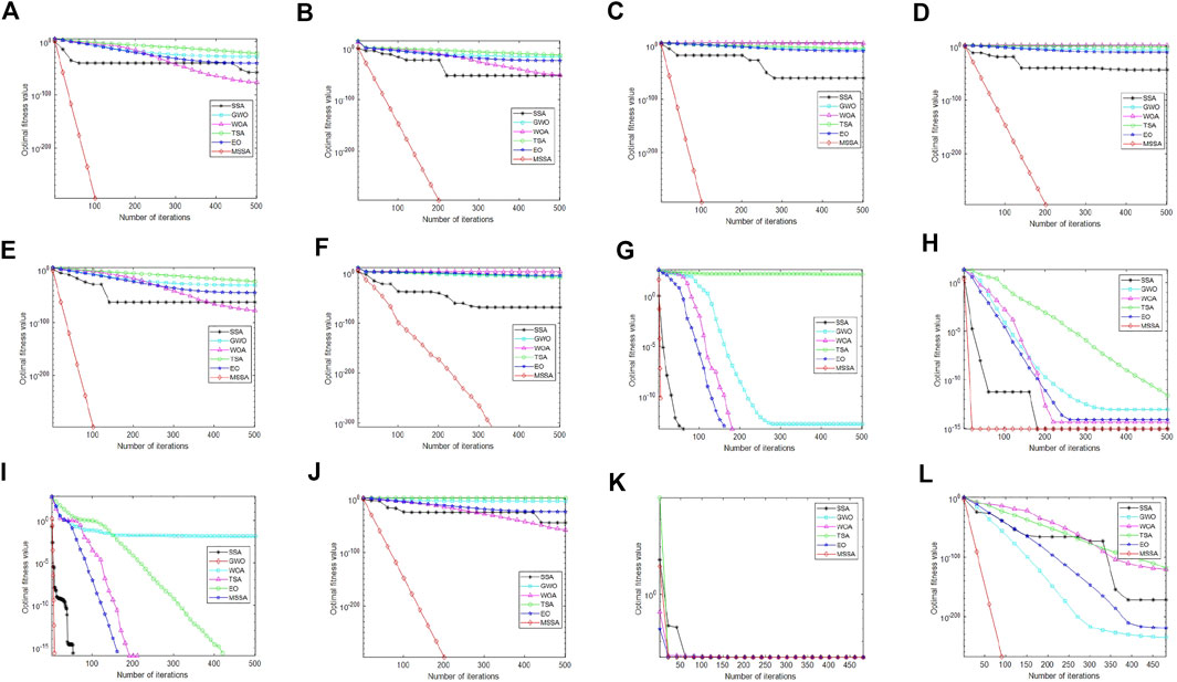
FIGURE 6. Comparison of optimization of each algorithm. (A) f1 mean convergence curve. (B) f2 mean convergence curve. (C) f3 mean convergence curve. (D) f4 mean convergence curve. (E) f5 mean convergence curve. (F) f6 mean convergence curve. (G) f8 mean convergence curve. (H) f9 mean convergence curve. (I) f10 mean convergence curve. (J) f11 mean convergence curve. (K) f13 mean convergence curve. (L) f16 mean convergence curve.
In general, only the mean and standard deviation are used for data analysis. The Wilcoxon rank-sum test is a non-parametric test method for the mean that is not limited by the overall distribution and has a wide range of applications (Derrac, J. et al., 2011). To more comprehensively analyze the performance difference between the MSSA and other algorithms, we selected the running results of MSSA and five comparison algorithms in sixteen test functions to conduct the Wilcoxon rank sum test. The p value can be considered to reject the null hypothesis when p < 5%, indicating that there is a significant difference in the test results. NaN indicates that there are no data to compare with the algorithm, +, =, and - indicate that the MSSA algorithm’s optimization performance is better than, equal to, and worse than the compared algorithms, respectively. The results of the Wilcoxon rank sum test are shown in Table 4:
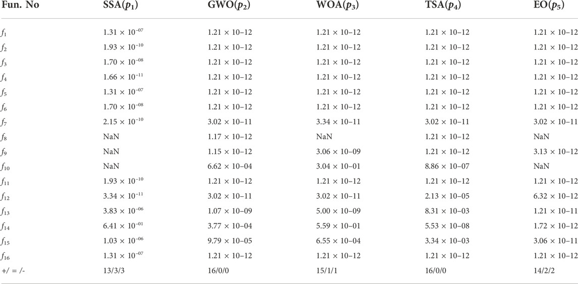
TABLE 4. Wilcoxon rank sum test results.
As seen from Table 4, the MSSA p value of the Wilcoxon rank sum test is less than 5%. The experimental results indicate that there is a significant difference between the MSSA and the other five algorithms, and the MSSA is significantly better than the others, further reflecting the robustness of the MSSA.
Most of the CEC2014 test functions (Tejani, 2018) are composed of the weights of multiple basic optimizations test functions, which makes the characteristics of the test functions more complex. In this paper, the proposed MSSA was tested against these complex test functions. On the one hand, these functions can effectively reflect the superior performance of MSSA for optimization of a complex function. On the other hand, the combinatorial optimization of multiple test functions reflects the applicability of SMSA to different complex optimization problems. To further test the performance of MSSA, this paper chose the CEC2014 single objective optimization function for solution analysis, including unit-modal, multi-modal, Hybrid, and composition type functions. Table 5 shows the relevant information of CEC2014 functions. This study compared the MSSA with five algorithms, including SSA, GWO, WOA, TSA, and EO. To ensure fairness of the algorithm comparison, the maximum number of iterations, Tmax = 1000, the population size was N = 30, and the dimension, dim = 30, were set to the same values in each algorithm, which were run 30 times independently, and the mean and standard deviation were recorded. The results are shown in Table 6.
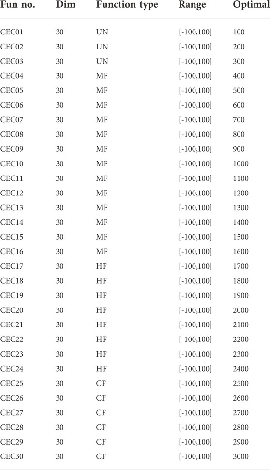
TABLE 5. Part of the CEC2014 function.
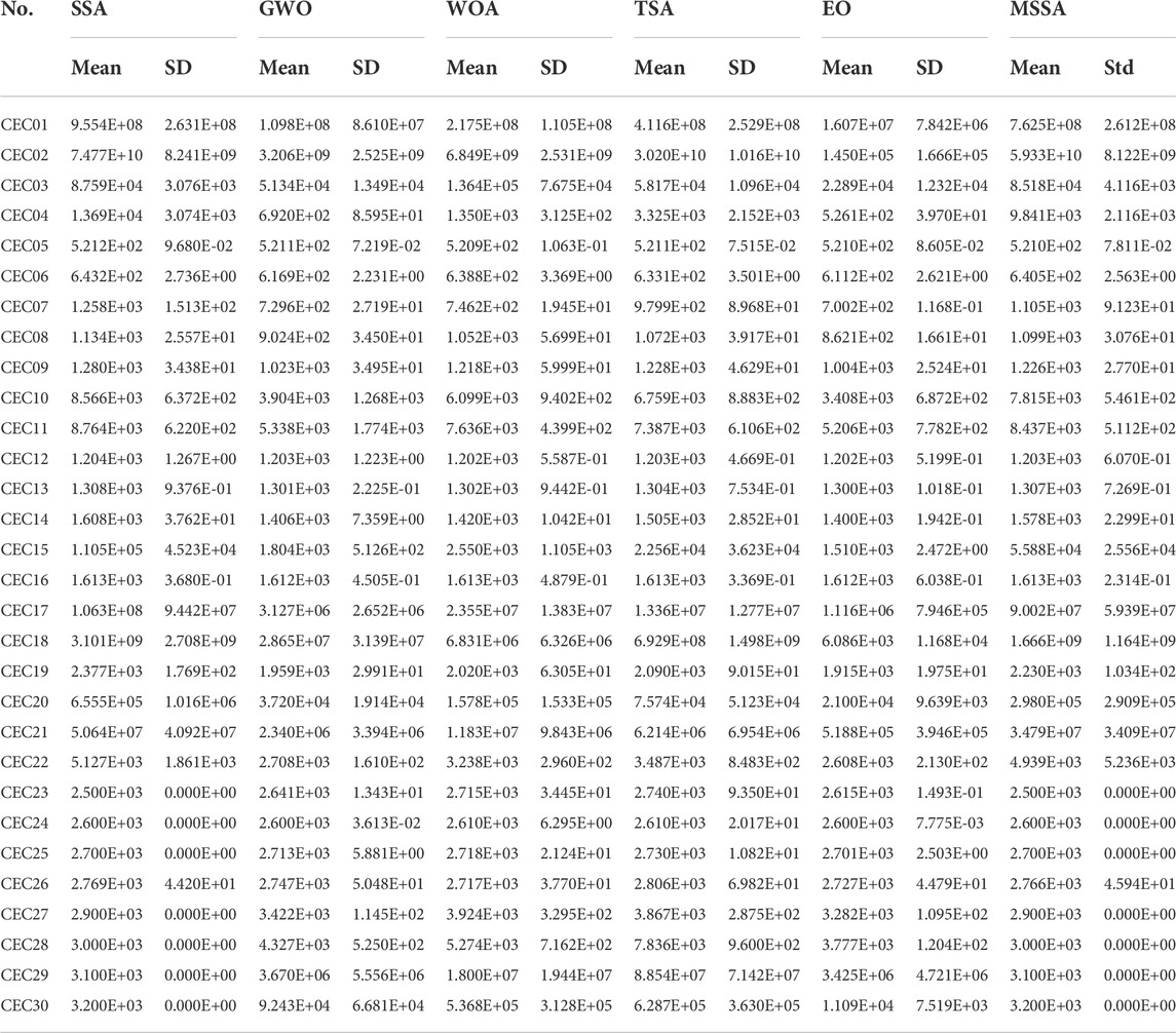
TABLE 6. CEC2014 function optimization comparison.
Table 6 shows that MSSA was better than SSA on 22 test functions, including CEC01, CEC02, CEC03, CEC04, CEC05, CEC06, CEC07, CEC08, CEC09, CEC10, CEC11, CEC12, CEC13, CEC14, CEC15, CEC17, CEC18, CEC19, CEC20, CEC21, CEC22, and CEC26. MSSA can find values close to SSA on CEC16, CEC23, CEC24, CEC25, CEC26, CEC28, CEC29, and CEC30. In terms of standard deviation, MSSA is better than SSA, GWO, and TSA on most test functions. It is worth noting that MSSA is better than SSA in the remaining 25 test functions except CEC03, CEC05, CEC16, CEC22, and CEC26. Generally, the proposed algorithm has more prominent advantages in the CEC2014 test function compared with the other eight algorithms.
In this section, we established two mathematical models of trajectory planning constraints in MATLAB and simulation experiments were carried out in a 3-D environment. This experiment combines the content of the above sections, and we conducted simulation experiments on UAV trajectory planning in two challenging mission environments. We compared MSSA with the SSA, BOA, WOA, and TSA to verify the performance improvement of the MSSA in the trajectory planning problem.
The first step in UAV trajectory planning was to initialize the relevant parameters. The basic parameters of SSA before and after the improvement were set as follows: the population size was N = 50, the maximum number of iterations was Tmax = 30, the proportion of discoverers was set to 20%, the scouter is 10%, and the alert threshold is set to 0.7.
To compare the performance of MSSA in the trajectory planning problem, we used two different map models as the task environment for simulation experiments. We built the three-dimensional environment and superimposed the threat area on it to make the model closer to the real environment. The area sizes of the two environments were 200×200×10 and 200×200×15 respectively. The start and end coordinates were set as S = (0, 0, 5) and E = (200, 200, 5). The height of the no-fly zone in the two environments was uniformly set at 10, the radius are R1 = [10; 8; 6; 7; 5] and R2 = [20; 15; 15]. The center coordinates were T1 = [115,161; 50,150; 90,20; 175,70] and T2 = [128,161; 50,150; 60,20]. The coordinates of the center of the mountain area were A1 = [48,41; 90,90; 162,96; 134,165; 30,135; 150,35] and A2 = [83,37; 149,36; 131,113; 54,118; 66,176; 131,178]. The heights were H1 = [7; 9;7; 6;6; 9] and H2 = [12; 8;7; 11; 6;9]. Slopes along the X axis direction were a1 = [25; 25; 35; 25; 25; 20] and a2 = [25; 25; 35; 30; 25; 20], and slopes along the Y axis direction were b1 = [25; 25; 30; 20; 30; 20] and b2 = [25; 35; 30; 35; 30; 20]. The 3-D environmental models are shown in Figure 7.
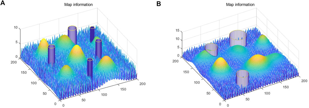
FIGURE 7. 3D map model information of two environments. (A) 3D map of environment 1. (B) 3D map of environment 2.
The trajectory simulation results of the two mission environments are shown in Figures 8 and 11, respectively. The two-dimensional trajectory planning results can be seen in Figures 9 and 12, respectively. The convergence graphs of the track cost function are in Figures 10 and 13, respectively. Figures 8 and 9 show that the five algorithms can both avoid the no-fly area from starting point to the target point in the environment. However, SSA, WOA, BOA, and TSA have large fluctuations. At the same time, the path is far away from the mountain peak and the no-fly area in the 2-D environment. This indicates that the algorithm falls into a local optimum when planning the trajectory. It is worth noting that the trajectory planned by MSSA is more stable, the fluctuation range is moderate, the trajectory is relatively stable, and it maintains a safe distance from the mountain and the threat area.
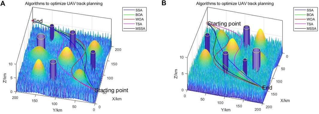
FIGURE 8. Simulation results of 3D trajectory planning in environment 1 from two different views.

FIGURE 9. Comparison of 2D track planning in environment 1.
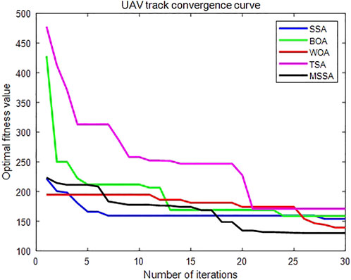
FIGURE 10. Convergence diagram of track cost function in environment 1.
In Figure 10, the SSA converges from the seventh iteration to the 27th iteration, indicating that the original SSA algorithm fell into a local optimum during the iteration. The values of BOA and TSA decreased rapidly at the beginning of the iterations, but fell into a local optimum many times in the later stage. In contrast, MSSA found the optimal value and jumped out of the local optima many times, which resulted in an ideal cost function value, thus demonstrating that MSSA can better avoid falling into local optima and find the best path.
Figures 11, 12 show that in the second task environment, the trajectories planned by the four comparison algorithms fluctuated greatly, which confirms the poor solution quality and insufficiency of these algorithms in complex trajectory planning. The MSSA is more stable, and it can be clearly seen that the path planned by the MSSA is the shortest. Figure 13 shows that MSSA’s optimal fitness values are lower than those of the comparison algorithms in the 8th iteration, and the local optimal value is still continuously removed at the end of the iteration. This shows that the trajectory cost function obtained by MSSA is smaller and the comprehensive performance index is better.
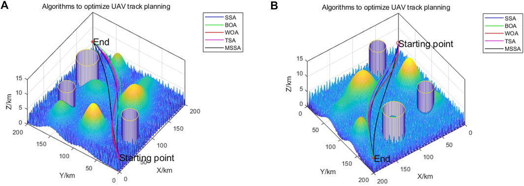
FIGURE 11. Simulation results of 3D trajectory planning in environment 2 from two different views.
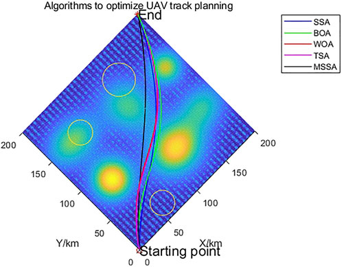
FIGURE 12. Comparison of 2D track planning in environment 2.
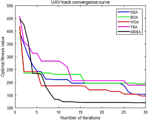
FIGURE 13. Convergence diagram of track cost function in environment 2.
To more objectively compare the performance of the MSSA with that of the other four algorithms in trajectory planning, this experiment used five algorithms to conduct 30 repeated experiments in two task environments. The population size was N = 30, and the maximum number of iterations was Tmax = 30. The experimental results are shown in Tables 7 and 8. The statistical results of the experimental data are shown in Tables 9 and 10. The performance of each algorithm was evaluated by comparing the optimal value, worst value, average value, and standard deviation of the track cost function values obtained.
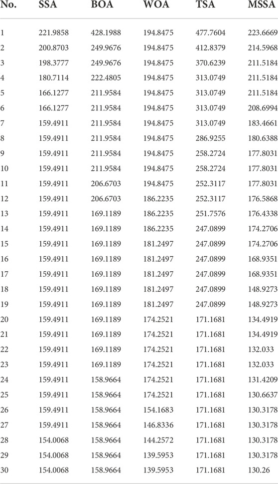
TABLE 7. Experimental data of environment 1.
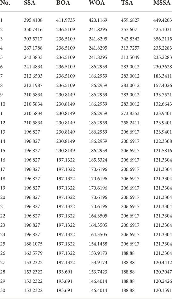
TABLE 8. Experimental data of environment 2.
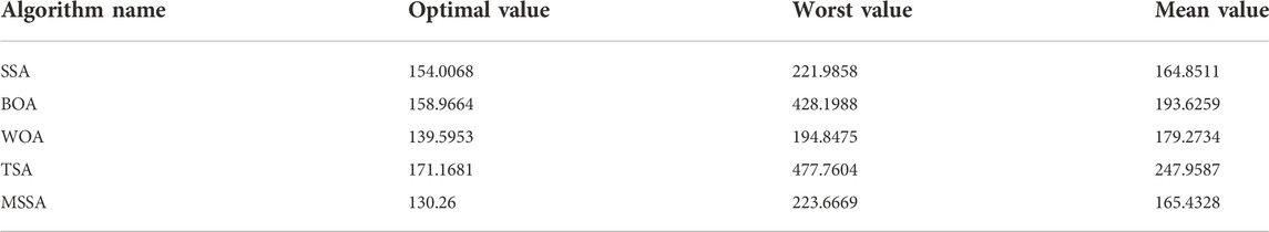
TABLE 9. Statistical data of experimental results in environment 1.
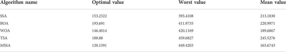
TABLE 10. Statistical data of experimental results in environment 2.
From Tables 9, 10, MSSA has obvious advantages in the performance of the UAV trajectory planning problem in the two environments. In the first environment, although MSSA is not the fastest in convergence, it did find the best value. In the second environment, MSSA was not only faster in convergence speed but also found the best value. The optimal values showed that the cost value of the MSSA for acquiring tracks was lower than that of the SSA, BOA, WOA, and TSA, illustrating that the MSSA had a stronger global search ability and higher convergence accuracy. The MSSA had a lower value than the other four algorithms on average, indicating that the MSSA had better trajectory planning quality and higher solution stability. In summary, the three improvement mechanisms proposed in this paper can effectively improve the algorithm global search ability, convergence accuracy, convergence speed and stability in terms of trajectory planning. The MSSA can balance the global search ability and local development ability of the algorithm and has excellent performance in solving complex multi-constraint combinatorial optimization problems such as UAV 3D trajectory planning. Thus, the trajectory planned by MSSA can meet the follow-up flight requirements for the UAV.
As one of the key technologies of the UAV autonomous control system, flight path planning is a hot research area in current information science. The UAV trajectory planning problem in a 3-D environment is complicated, computationally intensive and has many local optimal solutions, which poses great challenges to the performance of optimization algorithms. Based on analysis of the path planning problem and swarm intelligence algorithm, a new sparrow algorithm was proposed. First, the algorithm adopted a reverse learning strategy based on the law of refraction, enhanced the diversity of the algorithm, and improved the optimization accuracy of the algorithm. Second, the random step size of Levy’s flight boosted the local search capability of the algorithm. Lastly, the MSSA combined the fusion Cauchy mutation to increase the ability of the algorithm to jump out of local optima. We performed multiple ablation experiments in sixteen benchmark test functions with different characteristics. In the comparison of optimization performance of various improvement strategies and MSSA convergence experiments, the results indicated that Levy flight could help the population to deeply mine the global optimal values and improve the global search ability of the algorithm, proving that MSSA had greater stability and robustness than SSA.
In the comparison of convergence performance and high-dimensional performance with other algorithms, the results illustrated that MSSA had a significant competitive advantage and stability in solving complex, high-dimensional optimization problems. In addition, the Wilcoxon rank sum test and 30 CEC2014 complex functions were tested, and the results were compared with other metaheuristic algorithms and improved algorithms. The experimental results demonstrated that the improved MSSA algorithm had better stability, convergence accuracy, and optimization performance than other algorithms. Despite the significantly better performance demonstrated in this paper, the algorithm strategy could still be further improved. In subsequent work, refinements to the improved MSSA will be compared and analyzed with other advanced optimization algorithms to further improve the global search ability and local development ability of the algorithm.
An improved sparrow search optimization technique termed MSSA was proposed to increase the effectiveness of UAV trajectory planning in a three-dimensional environment. UAV trajectory planning simulation experiments were carried out in two different established three-dimensional geographic environments. The results showed that the path length of the obtained trajectory was considerably shorter while satisfying the constraints, further proving the feasibility and applicability of the proposed MSSA for trajectory planning in a three-dimensional environment. However, in this paper, the UAV simulation was simplified to a particle and a fixed flight speed was preset for solving the UAV path planning problem. In subsequent work, a more realistic UAV dynamics model should be established, and the flight restrictions of the UAV should be further studied. The UAV trajectory planning problem can be solved using the enhanced MSSA algorithm in subsequent work to significantly enhance the performance of complex environment trajectory planning from a variety of perspectives.
The original contributions presented in the study are included in the article/Supplementary Material, further inquiries can be directed to the corresponding authors.
QH and LY provided the idea of the article. YY wrote the article. YY derived the formula for the trajectory planning in the article. QH and LY were responsible for checking and improving the language in the article, and QH and LY provided all of the research funding.
The research was funded by the National Natural Science Foundation of China “Research on the Evidence Chain Construction from the Analysis of the Investigation Documents (No. 62166006)”, the National Natural Science Foundation of China “Rural spatial restructuring in poverty-stricken mountainous areas of Guizhou based on spatial equity: A case study of Dianqiangui Rocky Desertification Area (No. 41861038)”, and Guizhou Provincial Science and Technology Projects (Guizhou Science Foundation-ZK [2021] General 335).
The authors declare that the research was conducted in the absence of any commercial or financial relationships that could be construed as a potential conflict of interest.
All claims expressed in this article are solely those of the authors and do not necessarily represent those of their affiliated organizations, or those of the publisher, the editors and the reviewers. Any product that may be evaluated in this article, or claim that may be made by its manufacturer, is not guaranteed or endorsed by the publisher.
Abualigah, L., Yousri, D., Abd Elaziz, M., Ewees, A. A., Al-qaness, M. A. A., and Gandomi, A. H. (2021). Aquila optimizer: A novel meta-heuristic optimization algorithm. Comput. Industrial Eng. 157, 107250. doi:10.1016/j.cie.2021.107250
Bagherian, M., and Alos, A. (2015). 3D UAV trajectory planning using evolutionary algorithms: A comparison study. Aeronaut. J. 119 (1220), 1271–1285. doi:10.1017/S0001924000011246
Belge, E., Altanof, A., and Hacıoğlu, L. (2022). Metaheuristic optimization-based path planning and tracking of quadcopter for payload hold-release mission. Electronics 11 (8), 1208. doi:10.3390/electronics11081208
Chang, L., Shan, L., Jiang, C., and Dai, Y. (2021). Reinforcement based mobile robot path planning with improved dynamic window approach in unknown environment. Auton. Robots 45 (1), 51–76. doi:10.1007/s10514-020-09947-4
Derrac, J., Garcia, S., Molina, D., and Herrera, F. (2011). A practical tutorial on the use of nonparametric statistical tests as a methodology for comparing evolutionary and swarm intelligence algorithms. Swarm Evol. Comput. 1 (1), 3–18. doi:10.1016/j.swevo.2011.02.002
Dübel, S., and Schumann, H. (2017). Visualization of features in 3D terrain. ISPRS Int. J. Geoinf. 6 (11), 357. doi:10.3390/ijgi6110357
Fan, X., Sun, Z., Tian, E., Yin, Z., and Cao, G. (2022a). Medical image contrast enhancement based on improved sparrow search algorithm. Int. J. Imaging Syst. Technol. 123–23. doi:10.1002/ima.22794
Faramarzi, A., Heidarinejad, M., Stephens, B., and Mirjalili, S. (2020). Equilibrium optimizer: A novel optimization algorithm. Knowledge-Based Syst. 191, 105190. doi:10.1016/j.knosys.2019.105190
Hashim, F. A., Hussain, K., Houssein, E. H., Mabrouk, M. S., and Al-Atabany, W. (2021). Archimedes optimization algorithm: A new metaheuristic algorithm for solving optimization problems. Appl. Intell. (Dordr). 51 (3), 1531–1551. doi:10.1007/s10489-020-01893-z
Heidari, A. A., Mirjalili, S., Faris, H., Aljarah, H., Mafarja, M., and Chen, H. (2019). Harris hawks optimization: Algorithm and applications. Future gener. Comput. Syst. 97, 849–872. doi:10.1016/j.future.2019.02.028
Jia, Y., Zhou, S., Zeng, Q., Li, C., Chen, D., Zhang, K., et al. (2022). The UAV path coverage algorithm based on the greedy strategy and ant colony optimization. Electronics 11 (17), 2667. doi:10.3390/electronics11172667
Kaur, S., Awasthi, L. K., Sangal, A. L., and Dhiman, G. (2020). Tunicate swarm algorithm: A new bio-inspired based metaheuristic paradigm for global optimization. Eng. Appl. Artif. Intell. 90, 103541. doi:10.1016/j.engappai.2020.103541
Li, C., Zhang, N., Lai, X., Lai, X., Zhou, J., and Xu, Y. (2017). Design of a fractional-order PID controller for a pumped storage unit using a gravitational search algorithm based on the Cauchy and Gaussian mutation. Inf. Sci. 396, 162–181. doi:10.1016/j.ins.2017.02.026
Marini, F., and Walczak, B. (2015). Particle swarm optimization (PSO). A tutorial. Chemom. Intelligent Laboratory Syst. 149, 153–165. doi:10.1016/j.chemolab.2015.08.020
Mirjalili, S., and Lewis, A. (2016). The whale optimization algorithm. Adv. Eng. Softw. 95, 51–67. doi:10.1016/j.advengsoft.2016.01.008
Mirjalili, S., Mirjalili, S., and Lewis, A. (2014). Grey wolf optimizer. Adv. Eng. Softw. 69, 46–61. doi:10.1016/j.advengsoft.2013.12.007
Mohamed, N., Al-Jaroodi, I., Idries, A., and Mohammed, F. (2020). Unmanned aerial vehicles applications in future smart cities. Technol. Forecast. Soc. Change 153, 119293. doi:10.1016/j.techfore.2018.05.004
Momoh, J. A., Adapa, R., and El-Hawary, M. E. (1999). A review of selected optimal power ftow literature to 1993 Part I: Non linear and quadratic programming approaches. IEEE Trans. Power Syst. 14 (1), 96–104. doi:10.1109/59.744492
Olofsson, M., Andersson, G., and Söder, L. (1995). Linear programming based optimal power flow using second order sensitivities. IEEE Trans. Power Syst. 10 (3), 1691–1697. doi:10.1109/59.466472
Poli, R., Kennedy, J., and Blackwell, T. (2007). Particle swarm optimization. Swarm Intell. 1 (1), 33–57. doi:10.1007/s11721-007-0002-0
Price, K. V. “Differential evolution vs. the functions of the 2/sup nd/ICEO,” in Proceedings of the 1997 IEEE International Conference on Evolutionary Computation (ICEC '97), 153–157. April 1997 Indianapolis, IN, USA doi:10.1109/ICEC.1997.592287
Qadir, Z., Ullah, F., Munawar, H. S., and Al-Turjman, F. (2015). Addressing disasters in smart cities through UAVs path planning and 5G communications: A systematic review. Comput. Commun. 168, 114–135. doi:10.1016/j.comcom.2021.01.003
Salgado, R., Brameller, A., and Aitchison, P. (1990). Optimal power flow solutions using the gradient projection method. Part 1. Theoretical basis. IEE Proc. C Gener. Transm. Distrib. UK. 137 (6), 424–428. doi:10.1049/ip-c.1990.0057
Shin, J., and Bang, H. (2020). UAV path planning under dynamic threats using an improved PSO algorithm. Int. J. Aerosp. Eng. 2020, 1–17. doi:10.1155/2020/8820284
Tejani, G. G., Savsani, V. J., Patel, V. K., and Mirjalili, S. (2018). Truss optimization with natural frequency bounds using improved symbiotic organisms search. Knowl. Based. Syst. 143, 162–178. doi:10.1016/j.knosys.2017.12.012
Thompson, S. E., and Patel, R. V. (1987). Formulation of joint trajectories for industrial robots using B-splines. IEEE Trans. Ind. Electron. 34 (2), 192–199. doi:10.1109/tie.1987.350954
Tinney, W. F., Member, S., and Hart, C. E. (1967). Power flow solution by Newton’s method. IEEE Trans. Power Apparatus Syst. PAS-86(86), 1449–1460. doi:10.1109/TPAS.1967.291823
Van Steen, M., and Leiba, B. (2018). Smart cities. IEEE Internet Comput. 23 (1), 7–8. doi:10.1109/MIC.2018.2887182
Videras Rodríguez, M., Melgar, S. G., Cordero, A. S., and Márquez, J. M. A. (2021). A critical review of unmanned aerial vehicles (UAVs) use in architecture and urbanism: Scientometric and bibliometric analysis. Appl. Sci. (Basel). 11 (21), 9966. doi:10.3390/app11219966
Wen, X., Ruan, Y., Li, Y., Xia, H., Zhang, R., Wang, C., et al. (2022). Improved genetic algorithm based 3-D deployment of UAVs. J. Commun. Netw. 24 (2), 223–231. doi:10.23919/JCN.2022.000014
Whitley, D. (1994). A genetic algorithm tutorial. Stat. Comput. 4 (2), 65–98. doi:10.1007/BF00175354
Wu, C., Fu, X., Pei, J., and Dong, Z. (2021). A novel sparrow search algorithm for the traveling salesman problem. IEEE Access 9, 153456–153471. doi:10.1109/ACCESS.2021.3128433
Xue, J., and Shen, B. (2020). A novel swarm intelligence optimization approach: Sparrow search algorithm. Syst. Sci. Control Eng. 8 (1), 22–34. doi:10.1080/21642583.2019.1708830
Zhang, D., Xian, Y., Li, J., Lei, G., and Cang, Y. “UAV path planning based on chaos ant colony algorithm[C],” in Proceedings of the International Conference on Computer Science & Mechanical Automation (IEEE), 81–85. doi:10.1109/CSMA.2015.23October 2015 Hangzhou, China .
Zhang, W., Zhang, S., Wu, F., and Wang, Y. (2021). Path planning of UAV based on improved adaptive Grey wolf optimization algorithm. IEEE Access 9, 89400–89411. doi:10.1109/ACCESS.2021.3090776
Zhang, X., and Duan, H. (2015). An improved constrained differential evolution algorithm for unmanned aerial vehicle global route planning. Appl. Soft Comput. 26, 270–284. doi:10.1016/j.asoc.2014.09.046
Zhao, Y, J., Zheng, Z., and Liu, Y. (2018). Survey on computational-intelligence-based UAV path planning. Knowl. Based. Syst. 158, 54–64. doi:10.1016/j.knosys.2018.05.033
Keywords: smart cities, trajectory planning, improved sparrow search algorithm, UAV, three-dimensional
Citation: Yang Y, He Q and Yang L (2022) UAV trajectory planning based on an improved sparrow optimization algorithm with multi-strategy integration. Front. Environ. Sci. 10:1055807. doi: 10.3389/fenvs.2022.1055807
Received: 28 September 2022; Accepted: 01 November 2022;
Published: 28 November 2022.
Edited by:
Jiaxing Cui, Central China Normal University, ChinaReviewed by:
Jiqiang Niu, Xinyang Normal University, ChinaCopyright © 2022 Yang, He and Yang. This is an open-access article distributed under the terms of the Creative Commons Attribution License (CC BY). The use, distribution or reproduction in other forums is permitted, provided the original author(s) and the copyright owner(s) are credited and that the original publication in this journal is cited, in accordance with accepted academic practice. No use, distribution or reproduction is permitted which does not comply with these terms.
*Correspondence: Qing He, cWhlQGd6dS5lZHUuY24=; Liu Yang, bHlhbmczQGd6dS5lZHUuY24=
Disclaimer: All claims expressed in this article are solely those of the authors and do not necessarily represent those of their affiliated organizations, or those of the publisher, the editors and the reviewers. Any product that may be evaluated in this article or claim that may be made by its manufacturer is not guaranteed or endorsed by the publisher.
Research integrity at Frontiers
Learn more about the work of our research integrity team to safeguard the quality of each article we publish.