Non-steady-state closed dynamic chamber to measure soil CO2 respiration: A protocol to reduce uncertainty

Non-steady-state closed dynamic accumulation chambers are widely used to measure the respiration of terrestrial ecosystems, thanks to their low cost, low energy consumption and simple transportability, that allow measurements even in hostile and remote environments. However, the assessment of the accuracy and precision associated with the measurement system (independently of possible disturbances due to chamber-soil interactions) is rarely reported. This information is instead necessary for basic quality control, to compare data obtained by different devices and regression models and to provide Confidence Intervals (CIs) on the carbon flux values. This study quantifies the uncertainty associated with emission flux measurements, with a focus on very low fluxes. Calibration tests using different accumulation chambers and CO₂ sensors were performed, and fluxes were calculated by means of different models (parametric, non-parametric and flux models). The results of this work show that the linear regression model has the best reproducibility when compared to the other tested models, regardless of the sensor used and the chamber volumes, while the second order polynomial regression has the best accuracy. We remark the importance of building a calibration curve in the range of the expected flux values, with an interval between the lowest and highest imposed flux that should not exceed two orders of magnitude. To evaluate the reproducibility of the measurement, performing replicates for each imposed flux value is essential. We also show that it is necessary to carefully identify the best time interval for interpolating the CO₂ concentration curve in order to guarantee reproducibility and accuracy in flux estimates.

1 Introduction

Carbon dioxide (CO₂) uptake by photosynthesis and its release to the atmosphere by ecosystem respiration are the two fundamental processes determining the carbon balance of terrestrial ecosystems. Accurate CO₂ flux measurements are thus a prerequisite for understanding gas exchanges at the soil-vegetation-air interface and for quantifying the carbon budget.

There are several techniques to measure soil degassing (Lieth and Ouellette, 1962; Reiners, 1968; Kucera and Kirkham, 1971; De Jong and Schappert, 1972; Kanemasu, et al., 1974; Luo and Zhou, 2006). The most common techniques used for determining the contribution of soil respiration are based either on the use of accumulation chambers or on the concentration gradient. The accumulation chamber method does not require any assumption about the nature of the soil (Tonani and Miele, 1991).

In particular, the non-steady state Closed Dynamic Chamber (CDC) method, equipped with InfraRed Gas Analyser (IRGA), allows to measure the CO₂ concentration inside the chamber in real time (Parkinson, 1981; Norman et al., 1992). The CDC method is nowdays widely applied thanks to its low cost, low energy consumption and transportability that allow its use even in hostile and remote environments (Kutzbach et al., 2007; Pavelka et al., 2018).

The flux (Ø) under undisturbed conditions is calculated by means of the following equation (Healy et al., 1996; Kroon et al., 2008; Levy et al., 2011; Moffat and Brummer, 2017), which is valid for any gas:

$\varnothing =\frac{V}{A}{\left(\frac{dC}{dt}\right)}_{t=0}(1)$

where V and A are the volume and the base area of the accumulation chamber respectively, and dC/dt is the time derivative of the gas concentration evaluated at the starting time (t = 0). Therefore, the uncertainty of the flux measurement depends on the uncertainty of each of these factors (Jassal et al., 2012).

In Eq. 1, the time derivative of the gas concentration has to be obtained from fitting curves that are either empirical or based on diffusion theory (Venterea et al., 2015). The latter states that the increase of the gas concentration in the accumulation chamber over time should be represented by an exponential function when the diffusion is in quasi-steady-state condition (Hutchinson and Mosier, 1981), or by much more complex functions in case of non-steady-state flux (Livingston et al., 2006). For both stationary and non-stationary conditions, the models used for flux calculations based on diffusion theory are: (i) the HM model (Hutchinson and Mosier, 1981); (ii) the HMR model (Pedersen et al., 2010); (iii) the NDFE (non-steady state diffusive flux estimator) model (Livingston et al., 2006) and (iv) the CBC (Chamber Bias Correction) method (Venterea, 2010). The most used empirical models are: (a) the linear model (Beetz et al., 2013; Leiber-Sauheitl et al., 2013); (b) the second order polynomial model (Wagner et al., 1997); (c) the asymptotic model (Levy et al., 2011) and (d) the intercept method (Kroon et al., 2008). Levy et al. (2011) stated that the estimate of the flux has a large variability depending on the model chosen for interpolating the experimental data. An additional source of uncertainty is the choice of interpolation interval, identified by the starting and ending points, from which the derivative of the concentration curve is computed. The interpolation interval depends on the model chosen and can lead to important differences in the determination of the flux value under undisturbed conditions. The heterogeneity of the gas mixing ratio C in the accumulation chamber is another important source of uncertainty (Liu and Si, 2009; Hoffmann et al., 2015).

Finally, uncertainties can arise from the estimation of the volume or the V/A ratio. The volume (V) in the Eq. 1 is the effective system volume (V_e), which is larger than the chamber volume V_ch (Livingston and Hutchinson, 1995; Drewitt et al., 2002; Jassal et al., 2012). The Ve accounts for both the total volume of the measurement system (including the volume of the chamber, pump, IR measurement cell, connecting tube, and sample conditioning modules reported in Livingston et al., 2006) and the bias introduced by the model used for estimating the derivative. Therefore, it is characteristic of each instrumental setup and model used to fit the experimental curve, and it should be determined on a case-by-case basis.

Flux values are generally affected by both systematic and random measurement errors (Nay et al., 1994). Laboratory tests using known gas fluxes have been performed without distinguishing the variance generated by the measurement procedure from that related to the soil-instrument system (Reinhart et al., 1992; Nay et al., 1994; Gao and Yates, 1998; Evans et al., 2001; Butnor and Johnsen, 2004; Pumpanen et al., 2004; Nomura et al., 2019). Despite the widespread use of the CDC method, the accuracy and precision of flux measurements associated with the instrumental apparatus, independent of the interaction with the soil, are rarely reported (Heinemeyer and McNamara, 2011). However, this information is necessary to set up standardized quality controls, to perform statistical comparisons between models and data, and to provide Confidence Intervals (CIs) on carbon budgets (Savage et al., 2008).

Motivated by this need, here we quantify the uncertainty of the flux measurements using the CDC technique, with special attention for the case of very low gas fluxes such as those met in high-altitude or high-latitude ecosystems. To this end, calibration tests using different accumulation chambers and CO₂ sensors were performed. These tests have been designed to: i) set a calibration procedure that allows to compare measurements performed with different instrumental settings; ii) identify the most suitable procedure to account for the effective volume V_e; iii) assess the variability of the derivative (dC/dt) estimates associated with the choice of the lower and upper limits of the interpolation interval (i.e., the interpolation range); iv) choose the best flux estimation model.

2 Materials and methods

2.1 Experimental setup

The experimental laboratory tests were performed by measuring CO₂ concentration vs. time inside a CDC accumulation chamber placed on a rubber-covered table (calibration table, CT). At the center of the CT, the outlet of a 2 mm diameter Rislan tube was connected to a cylinder by means of two Alicat Scientific^® mass flow controllers (MFC) characterized by different working ranges: 1–10 scc/min (standard cubic centimeters per minute), and 5–1,000 scc/min. Both MFC have accuracy and repeatability of ±2% of Full Scale (FS). The cylinder contains a standard certified mixture of 2% v/v of CO₂ (balance N₂). The instrumentation setup is shown in Figure 1.

FIGURE 1

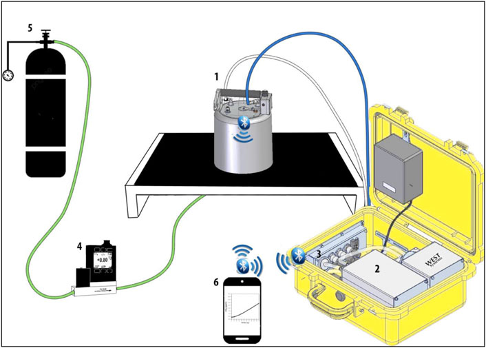
FIGURE 1. Instrumental set-up: 1) a steel/aluminium cylindrical accumulation chamber with known volume and base surface, equipped with a pressure compensation device to maintain pressure equilibrium between inside and outside the chamber, and a fan with a speed of 80 rpm to avoid errors due to air stratification and to ensure efficient headspace mixing during the measurement; 2) the IRGA analyser for CO₂ measurements; 3) a pneumatic system comprising a membrane pump (2.5 l/min) and pipes to transport the gas from the chamber to the gas detectors and back to the chamber; 4) mass flow controller (MFC); 5) gas cylinder with known CO₂ concentration; 6) a palmtop computer connected to the instrument through the Bluetooth wireless standard. All these “devices” are connected to each other.

The tests were conducted using two Non-Dispersive InfraRed (NDIR) gas analyzers having different accuracy and Root Mean Square (RMS) noise:

i) A gas analyzer, named L in the following, with measurement range 0–20,000 ppmv, accuracy higher than 1.5%, RMS noise at 370 ppmv less than 1 ppmv (LI-COR 840; LI-COR Inc.);

ii) A gas analyzer, named V in the following, with measurement range 0–20,000 ppmv, accuracy about 2%, RMS noise at 370 ppmv of 3 ppmv (GMP 343, Vaisala).

The measurements were performed using two cylindrical accumulation chambers characterized by different volume and base area:

1) Chamber A, with a volume of 2.770 10^–3 m³ and a base area of 30.8 10^–3 m²;

2) Chamber B, with a volume of 6.186 10^–3 m³ and a base area of 31.7 10–3 m².

The volume of the recirculating system provided with the sensor, V and L, was 0.284 10^–3 m³ and 0.216 10^–3 m³, respectively. Hence, the total volumes (chamber plus recirculating system) were: 3.054 10^–3, 6.470 10^–3, 2.986 10^–3, and 6.402 10^–3 m³ for the measurement system V + A, V + B, L + A and L + B, respectively.

The imposed CO₂ fluxes used for the experimental tests were 0.02, 0.1, 0.2, and 1 scc/min. For each combination of flux value, chamber type and sensor, 10 replicates were performed (for a total of M = 160 measurements).

The recording of CO₂ concentration inside the chamber started at the placement of the chamber on the CT (Figure 1) and was stopped after 120 s. The CO₂ concentration inside the chamber was recorded every second, thus providing 120 concentration values for each measurement run. Between the different measurement runs, the apparatus was purged with ambient air in order to clean it from the excess CO₂. The measurement dataset is reported in the Supplementary Material.

2.2 Models

The CO₂ fluxes were obtained from the measurements of CO₂ concentration vs. time using the interpolation models described in the Supplementary Material (SM). We tested: i) the linear model (Naganawa and Kyuma, 1991); ii) the 2^nd order polynomial model (Wagner et al., 1997); iii) the asymptotic model (Levy et al., 2011); iv) the intercept model; v) the HM model (Hutchinson and Mosier, 1981); vi) the Theil-Sen (T-S) method (Hollander and Wolfe, 1999); vii) the HMR model (Pedersen et al., 2010). The models (i) to (vi) provide an estimate of the concentration derivative (dC/dt) at time t = 0 (∂_t=0), while the outcome of the model (vii) is the direct flux estimation.

The HM model, in particular, is based on Eq. 2 (further details in the SM):

${\mathfrak{f}}_0=\frac{V}{A}\left(\frac{1}{t_1}\frac{{\left(C_1-C_2\right)}^2}{2C_1-C_2-C_0}\mathit{Ln}\left[\frac{C_1-C_0}{C_2-C_1}\right]\right)\to {\mathfrak{f}}_0=\frac{V}{A}C(2)$

where C represents the constant of proportionality between the flux and the V/A ratio that should be determined empirically, C₀ the gas concentration at time t = 0, C₁ the gas concentration at time t₁, and C₂ the gas concentration at time t₂.

2.3 Data processing

The experimental workflow is shown in Figure 2. First, the different calculation models were compared in the whole 120 s acquisition interval (Section 3.1), for each of the M = 160 measurements (4 chamber + sensor combinations, four set fluxes, 10 replicates for each chamber + sensor combination and imposed flux). Second, the parametric [i.e., (i–iii)] and non-parametric [i.e, (iv) and (vi)] models, which may depend on the number of experimental data, were applied to subsets of measurements with size N, N-1, … to N-N/2, where N = 120 is the total number of CO₂ concentration values acquired during each measurement (Sec. 3.2). These subsets were built by taking the first, second, third, … to N/2–1 acquired data as a starting point for the interpolation. For each of the M = 160 measurements we obtained 60 subsets of different length, for a total of 9,600 subsets. Third, for the parametric models (linear, 2nd order polynomial and asymptotic regressions), we also assessed the variability of the estimated mean derivative of the CO₂ concentration by considering different temporal intervals. Once we tested the variability obtained by choosing different starting points, as explained above, the best ending point has been identified. To this end, we estimated the mean derivative starting from an interval of 30 s and then adding one second at each step. This was repeated for each of the M = 160 measurements.

FIGURE 2

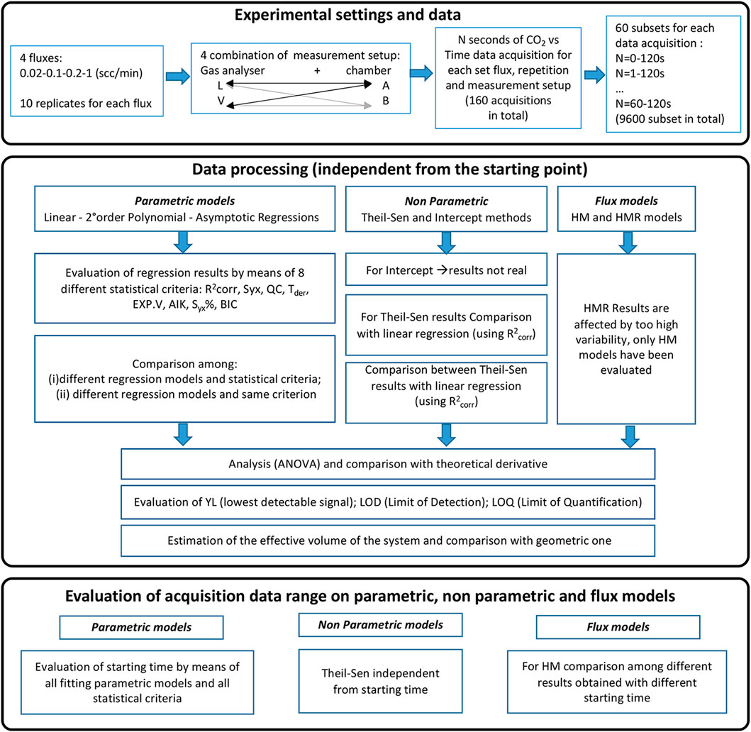
FIGURE 2. Schematic diagram of the workflow.

2.4 Statistical criteria

The models were evaluated by the statistical criteria reported in Table 1. The main statistical parameters (mean, median, 1st and 3^rd quartile, maximum and minimum value) are shown by means of box-whiskers diagrams. The Interquartile Ranges (IQR) have been used for comparing the derivatives obtained by the different models. Median values obtained from the parametric models were compared using the Two Sample Hypothesis Testing by Wilcoxon-Mann-Whitney (WMW) (Bain and Engelhardt, 1992). After verifying normality using QQ-plots, the presence of outliers was identified by means of the Grubbs test (Grubbs and Beck, 1972; Massart et al., 1997). A t-test (Crow et al., 1960) was used to investigate whether the observed differences between the slopes of the calibration curves provided by the different models were due to random measurement errors or to systematic effects.

TABLE 1

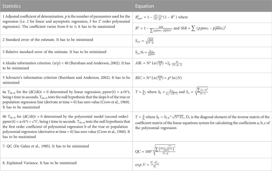
TABLE 1. Statistical criteria used to evaluate models.

The proportionality between the derivative values and the imposed fluxes was verified by means of Pearson’s linear correlation coefficient (R) to test the null hypothesis R = 0 (equal-tail test) at 0.05 significance level. When R was significantly different from 0, the linear regression between the derivative (dependent variable) and the imposed flux (independent variable) was constructed using the least squares method. The lack of fit of the regression curve was tested by analyzing the residues with ANOVA and evaluating the ratio F between the lack of fit and the pure error (F-test, Draper and Smith, 1981). The lowest detectable signal (YL), the LOD (Limit Of Detection) and LOQ (Limit Of Quantification) of the system used for flux measurement were determined using the method reported by Massart et al. (1997) and Meier and Zünd (2000).

Data processing was performed by the software STATISTICA 10^©.

3 Results

3.1 Model comparison

3.1.1 Parametric models

The parametric models provided different values of the median and interquartile range for ∂_t=0 (Supplementary Table S1). For the linear and asymptotic models, the interquartile intervals were equivalent, whatever statistical criteria were used for fitting model parameters (Table 1). For the polynomial model, in contrast, the interquartile intervals varied greatly with the adopted criterion. Regardless of the type of sensor, accumulation chamber and statistical criterion used, the estimated ∂_t=0 was in general lower than the imposed flux value for all parametric models (Supplementary Figures S1A, B; S2). The two sensors, even if coupled to the same chamber, produced significant differences in the ∂_t=0 values.

Figure 3 shows the ∂_t=0 values versus the imposed fluxes for the different measurement systems. The calibration curves obtained for the same measurement system showed different slopes, depending on the model used for estimating the derivative. The correlation coefficients of the calibration curves, excluding outliers, revealed that all linear correlations between the estimated derivatives and the imposed fluxes were significantly different from 0 (according to Pearson’s linear correlation coefficient).

FIGURE 3

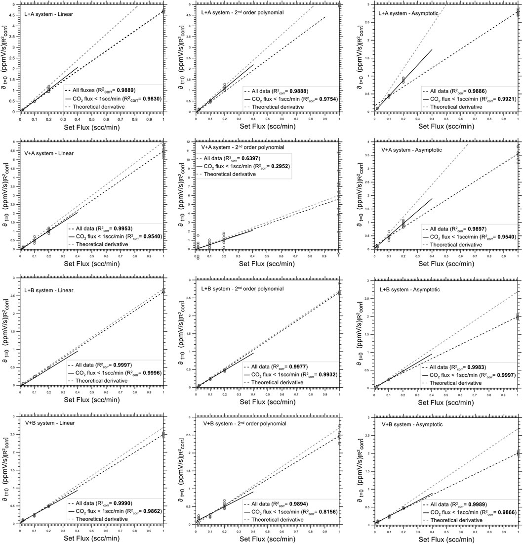
FIGURE 3. Set flux values versus ∂t=0 for the different measurement setups (chamber+sensor) and for different parametric regression models. The black dotted line refers to all data; the black solid line is obtained using only the fluxes lower than 1scc/m; the dotted grey line represents the theoretical derivative. The R²corr values are also reported.

A t-test was used to investigate whether the observed differences between the slopes of the calibration curves provided by the three different parametric models were due to random measurement errors or to systematic effects. The t-test results for fluxes lower than 1 scc/min are reported in Table 2. Statistically significant differences between the slopes estimated using the linear, second order polynomial, and asymptotic models are shown in bold. No significant differences (t-test, 0.05 significance level) were detected using the A chamber and the V sensor.

TABLE 2

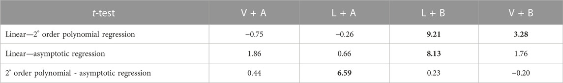
TABLE 2. The t-test results to verify the null hypothesis H0: the differences between the slopes of the calibration curves are equal to 0. Flux < 1scc/min. Bold values denote statistically significant ones.

Analysis of variance (ANOVA) was then applied to test whether the parametric models used to construct the calibration curves were affected by lack of fit. The results of the ANOVA on all data, excluding outliers and the highest flux (1 scc/min), are reported in Table 3. When we used all the imposed fluxes, the linear relationship between flux and derivative estimated using the asymptotic model always showed a lack of fit (Lof) for all systems. In contrast, the ANOVA indicated that, using fluxes <1 scc/min, the calibration curves for the L + B and V + A systems showed no Lof whatever method was used, whereas for the V + B system they showed a Lof for all three models. When the calibration curves were constructed using only fluxes lower than 1 scc/min, the intercept was not significantly different from 0 (at 0.05 significance level) only for the L + B system using the linear model, and for the V + B system using all fitting models.

TABLE 3

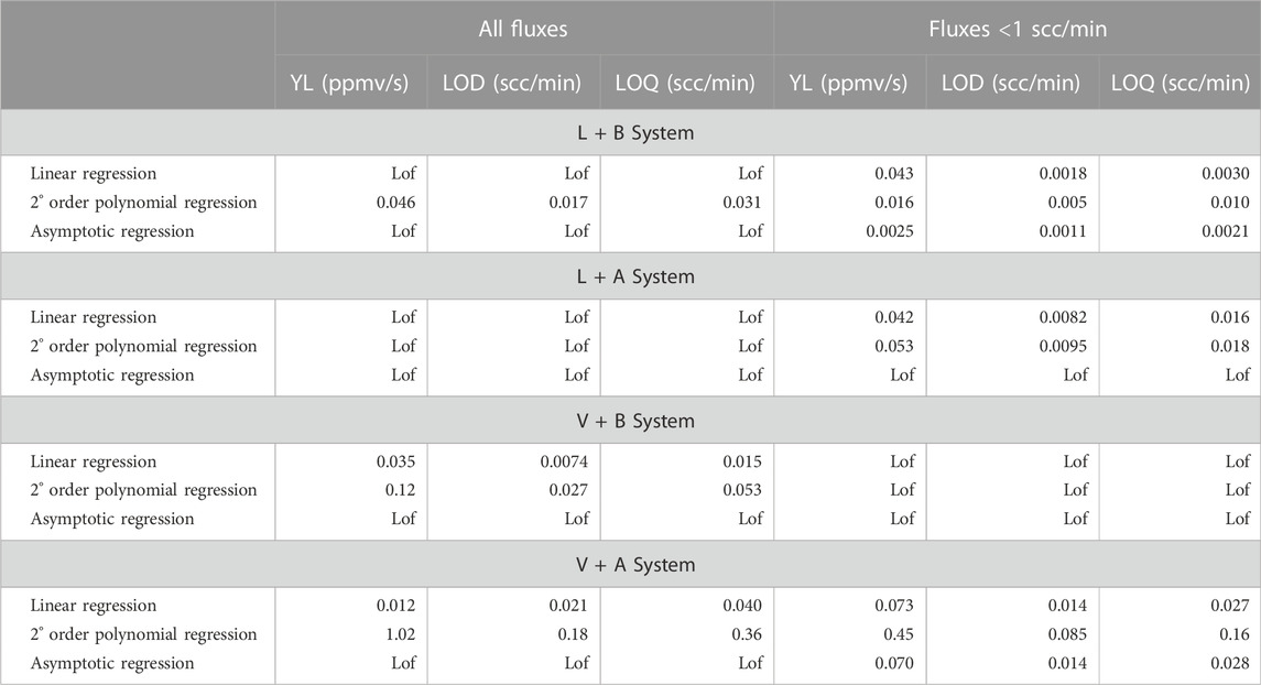
TABLE 3. Lowest detectable signal (YL), limit of detection (LOD), and limit of quantification (LOQ), values for the three types of regression and for different instrument combinations. Lof = Lack of fit.

Table 3 shows that the V sensor always had higher detection limits than the L sensor, for the same accumulation chamber. The A chamber always showed a higher detection limit than the B chamber. In general, the detection limit was lower when using the value of ∂_t=0 obtained from linear regression. The YL, LOD and LOQ limits obtained by calibration curve including fluxes lower than 1 scc/min were smaller than those calculated by calibration curve with all imposed fluxes. The detection limits obtained with linear and asymptotic regression were comparable and lower than those obtained by polynomial regression.

Finally, in order to estimate the difference between V_ch and V_e and how this difference depends on the parametric model and/or on the chosen criterion, we compared the volumes obtained after removing the outliers by the median values of ∂_t=0 calculated for each of the 10 measurements for a given flux. The asymptotic regression provided the highest V_e median values, whatever the statistical criterion used. The different behavior of sensor V compared to sensor L must be noted, especially when the ∂_t=0 values were estimated using the 2nd order polynomial regression (see Supplementary Table S2).

3.1.2 Non-parametric models

In many cases, ∂_t=0 values statistically compatible with zero were obtained using the intercept model, especially for low fluxes and the V sensor. Consequently, the linear relationship between the logarithm of the derivative and time (see SM Eq. 2) cannot be used.

The T-S model applied to ∂_t=0 provided results that were comparable with those obtained by linear regression, using $R_{corr}^2$ as a statistical criterion (Figure 4). However, deviations were detected in case of high fluxes using the V + A system, for which the derivative values obtained by linear regression were larger than those obtained using the T-S method. Figure 5 shows that the correlation between the derivatives and the imposed fluxes, either including or excluding 1 scc/min fluxes, was always larger than zero, regardless of the instrument used. For fluxes lower than 1scc/min, the $R_{corr}^2$ values were always larger than 0.977 for the L + A, L + B and V + B systems, and $R_{corr}^2=0.94$ for the V + A system.

FIGURE 4

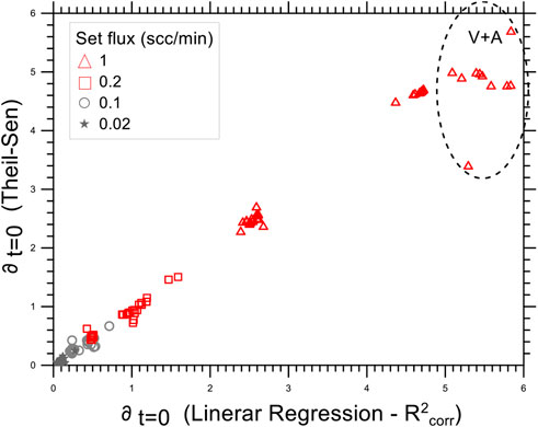
FIGURE 4. Binary diagrams comparing the ∂t=0 by the T-S method and those obtained by linear regression (maximizing R²corr). Point types correspond to different set fluxes. All replicates obtained for each set flux value and all measurement setup combinations (chamber+sensor) were used.

FIGURE 5

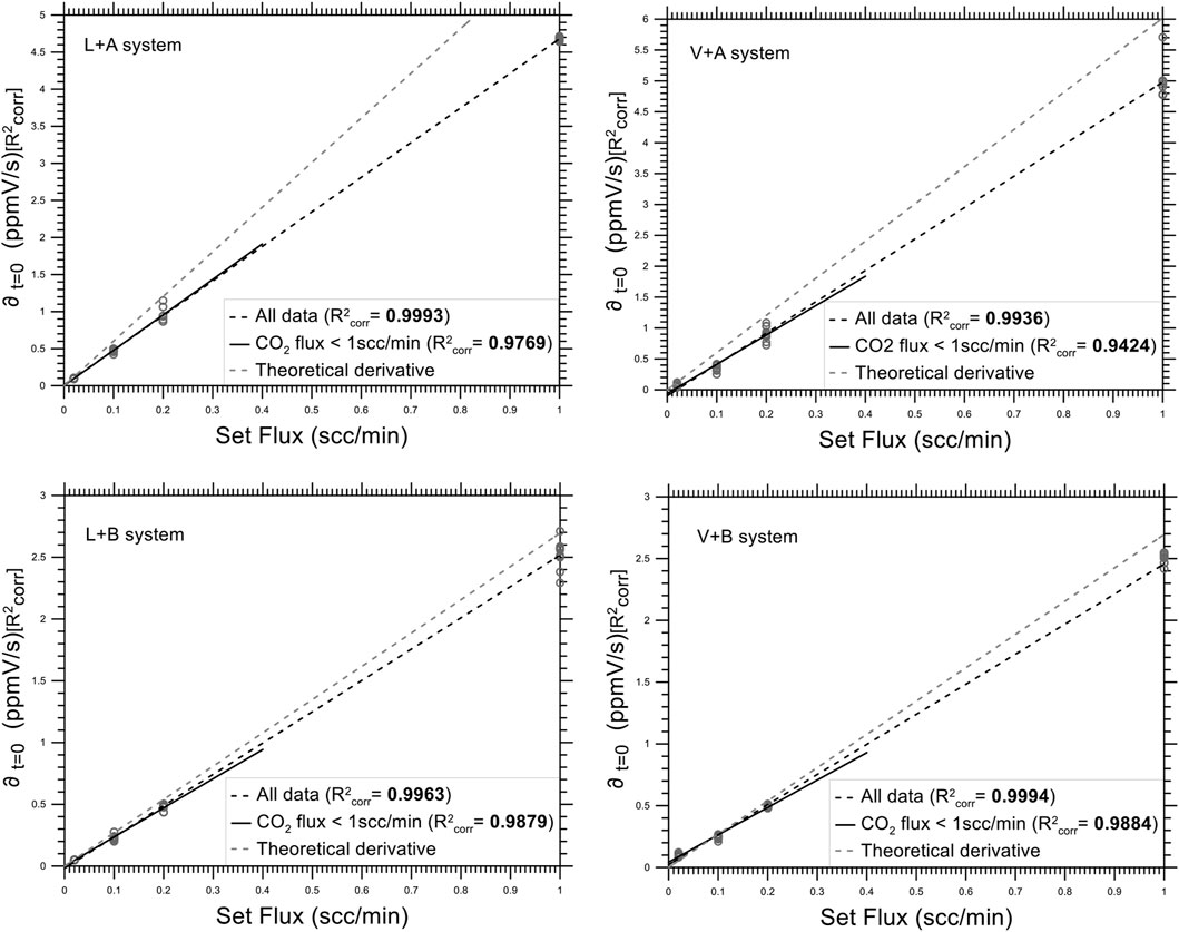
FIGURE 5. Set fluxes values versus ∂t=0 calculated with the TS method for the different measurement setups systems (chamber+sensor). The black dotted line refers to all data; the black solid line is obtained using only the fluxes lower than 1scc/m; the dotted grey line represents the theoretical derivative. The R²corr values are also reported.

The results of the ANOVA analysis (Table 4) indicated that the L + A and L + B systems had no lack of fit, while the V + B system had lack of fit whatever flux range was considered, and the V + A system had no lack of fit only for the range of fluxes that include 1 scc/min. All the regression lines that were not affected by lack of fit had the intercept compatible with 0 (at 0.05 significance level). Table 4 shows that the limit values YL, LOD and LOQ for the L + B system are lower for flux values below 1 scc/min with respect to the ones obtained for higher flux values.

TABLE 4

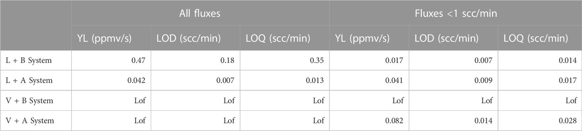
TABLE 4. YL, LOD, and LOQ values for the different types of measurement system calculated using TS model.

The difference between V_ch and V_e was evaluated also in this case. The median values of the effective volumes based on the experimental derivatives, calculated using the T-S method, were comparable with those determined using the parametric models and they were all higher than V_ch (Supplementary Table S2).

3.1.3 Flux models

In the HM model, the value of the constant of proportionality between the flux and the V/A ratio, C, was obtained by considering the median of all values in the subsets, and it can be directly compared to the value of the derivative obtained by the parametric models. The value of C showed significant variation (using the WMW test) in all systems for all the different imposed flux values (T median values of the Supplementary Table S2). In general, the median values of C were comparable with the ∂_t=0 medians estimated using the 2^nd order polynomial and linear regression models, but the interquartile intervals of the C values were significantly larger than the values of the derivatives calculated using the parametric models. The correlation $R_{corr}^2$ between flux values and the C terms are shown in Figure 6. The values of $R_{corr}^2$ are all significantly different from zero, so it was correct to build calibration straight lines using the least squares technique.

FIGURE 6

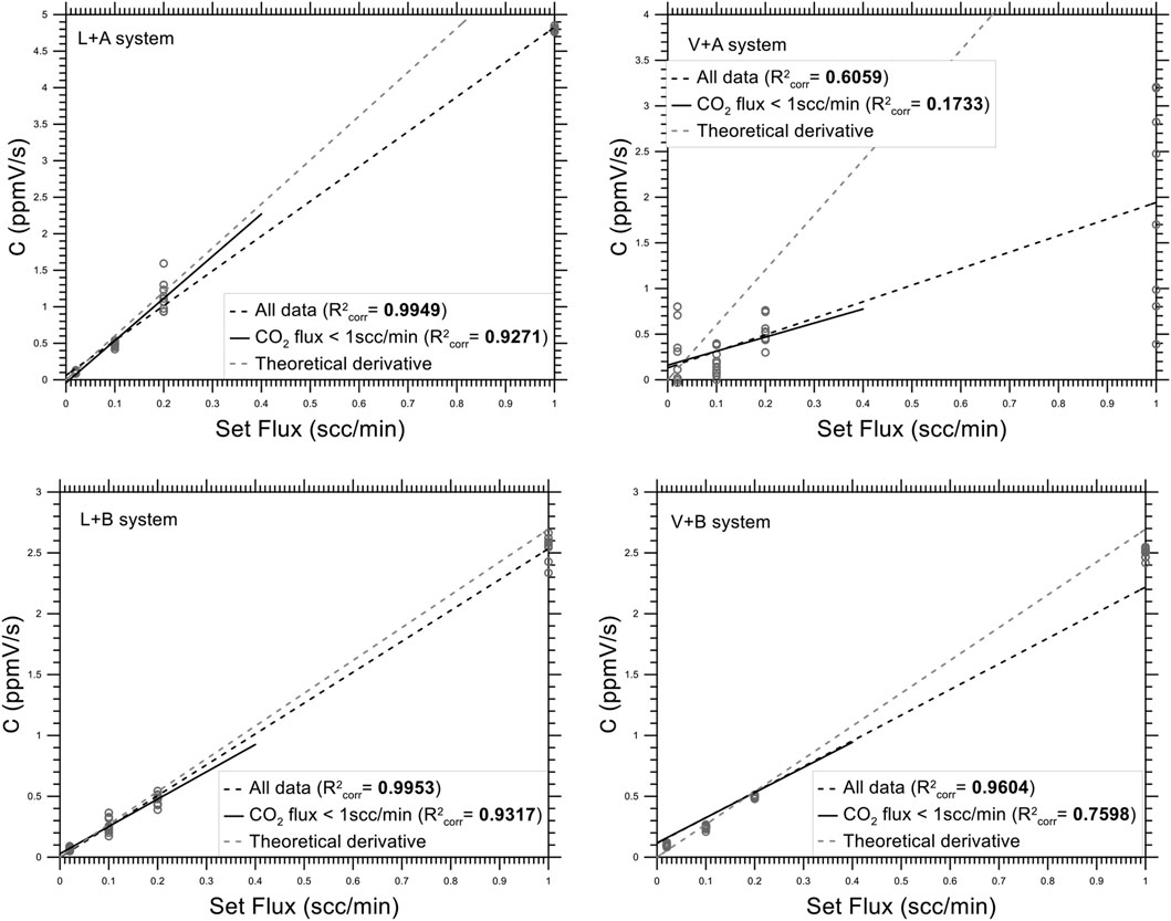
FIGURE 6. Set fluxes values versus term C calculated with the HM models (Eq. S3) for the different measurement setups (chamber+sensor). The black dotted line refers to all data; the black solid line is obtained using only the fluxes lower than 1scc/m; the dotted grey line represents the theoretical derivative. The R²corr values are also reported.

The ANOVA analysis results (Table 5) indicated that the calibration curves calculated using all fluxes showed lack of fit for the L + A and L + B systems; this was not the case when considering only fluxes <1 scc/min. The intercepts of the calibration curves were significantly different from zero for the L + A, L + B and V + A systems, but not for the V + B system. As illustrated in Table 5, the L + A and L + B systems had the same LOQ. Also, Ve is larger than Vch for both chambers (Supplementary Table S2).

TABLE 5

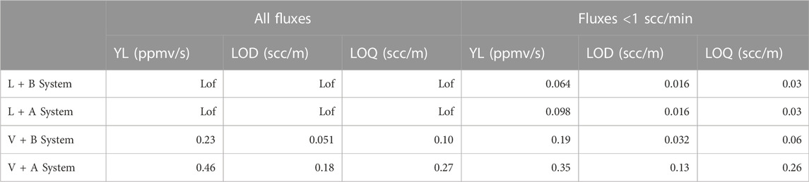
TABLE 5. YL, LOD, and LOQ values for the different types of measurement system calculated by HM model.

The HMR model gives directly the flux values by using the concentration values at time t, c_(t), which depends on f, k and Ø₀ (see SM Eq. 4). These parameters were computed using a non-linear system of equations and their convergence values varied greatly with the initial tentative solutions, especially in the case of low fluxes. This large variability indicates that this method is not robust for our purposes.

3.2 Influence of the interpolation time range

First, we consider the lower limit, that is quite critical. Figure 7 and Supplementary Figure S3 show examples of how the derivative value changes as a function of the chosen lower limit of the estimation time range, keeping the upper limit at 120 s. By using the 2^nd order polynomial regression, the value of the derivative varied greatly with the variation of the lower limit, while this issue did not emerge using the linear regression.

FIGURE 7

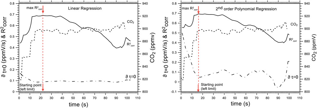
FIGURE 7. Trend of the ∂t=0 calculated using linear (left) and 2° order polynomial (right) regressions as a function of the choice of the left limit (best approximating t=0). The value of R²corr is also reported, as well as the identified starting points and the measured CO₂ concentration versus time.

The T-S model will not be discussed here, as it is independent of the choice of the lower interpolation limit.

For the HM model, derivative estimates varied greatly with the value of the lower limit. Figure 8 reports the maximum and minimum values, the median and the interquartile interval of all the estimates for each selected range, obtained by varying the time t₀ (lower limit) and therefore C₀. It should be noticed that when t₀ was between 13 and 25 s after the start of measurements, the values of the median of the C term were close to the theoretical derivative. Hence, considering all results, we obtained different estimates and there was no definite statistical criterion for the choice of the optimal lower limit of the interpolation range.

FIGURE 8

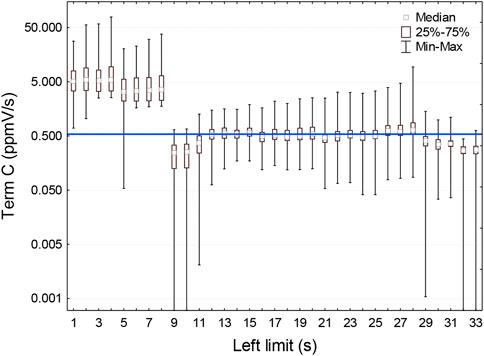
FIGURE 8. Calculation of ∂t=0 for each subset obtained by using the HM method and changing the upper limit of the interpolation interval. The median, interquartile, minimum and maximum values for each replicate and for a given set flux are reported. The X-axis shows, for each subset, the value of the left limit (approximating t=0) that characterizes the subset. The blue line represents the theoretical derivative.

A further point concerns the value of the upper limit to the interpolation range, using the same lower limit. Here we consider: a) An upper limit for which the value of $R_{corr}^2$ is maximum, and b) an upper limit coincident with the final experimental acquisition time (Supplementary Table S3). The comparison showed that for the L + A system there were no significant differences between the results for all types of regression used. For the L + B system, there were no significant differences using the linear regression, while using the 2nd order polynomial regression the derivative estimates obtained using the final acquisition time as upper limit were always larger than those obtained using the upper time limit that maximizes $R_{corr}^2$. For the V + A system, the mean values of the derivatives estimated with the linear and asymptotic regression were comparable for flux values larger than 0.02 scc/min. When using the 2^nd order polynomial regression with flux values <1 scc/min, the derivatives estimated by maximizing $R_{corr}^2$ were always lower than those obtained using the upper limit equal to the final acquisition time. For the V + B system, the two estimation procedures led to different results only in the case of fluxes of 0.02 scc/min, regardless of the type of regression used. In several cases, however, the value of the standard deviation on the estimated derivative can be so large that it is not possible to discard the null hypothesis that the mean values are equal (at 0.05 significance level).

4 Discussion

4.1 Measurement reproducibility

The reproducibility of the ∂_t=0 values varied depending on the interpolation model adopted and the measurement system used.

The 2nd order polynomial regression showed the most marked variability of ∂_t=0 values, while the asymptotic or linear regressions displayed smaller variability. For each measurement system, the largest variability in the estimates of the derivatives was observed for the highest values of the imposed flux, at 1 scc/min. Comparing the various instrumental setups, the main differences in the Interquartile Range were observed for fluxes of 0.02 scc/min. The results obtained by using different statistical criteria, as reported in Table 1, indicate that the variations of the median values of the derivative estimated using the 2nd order polynomial regression were larger than those obtained by the asymptotic and linear regression. For the linear regression, the percentage of IQR with respect to the median value was close to 10% when using the V sensor and an imposed flux of 0.02 scc/min; in all the other cases it was always less than 5%, with values for the L sensor lower than those for the V sensor. Using the 2nd order polynomial regression for data acquired with the V sensor led to variations that can be larger than 100% when the flux is 0.02 scc/min. For higher fluxes, the variations remained larger than 30% (the largest variations always occurred when using chamber A).

The L and V sensors showed different behaviour also using non-parametric models (T-S model) and the flux model (HM). In general, the IQR of the derivatives estimated using the HM model were larger than those determined by linear regression. The derivatives estimated on data acquired with the V sensor were more variable than those obtained when using the L sensor. This can be attributed to the different RMS of the two sensors.

The volume of the accumulation chamber played a relevant role in determining the reproducibility of the measurements. The reproducibility of the derivative calculation, and consequently of the flux value, is evaluated through 10 replicates of the same measure. Supplementary Table S3 shows that the chamber with smaller volume is characterized by standard deviation and IQR values of the derivative that are higher than those obtained for the chamber with larger volume, considering the same sensor and the same model for derivative calculation.

The reproducibility of the measurements obtained by using two different sensors and accumulation chamber volumes can be estimated by the number of measurements to be taken in order to have the same 95% confidence interval for the mean value of the flux. For the case of ∂t = 0 estimated by linear regression and fluxes of 0.02 scc/min, 178 repetitions were necessary for the V + B system to obtain the same confidence interval as that obtained with 10 replicates using the L + B system. For the V + A system, it would take 70 repetitions to have the same confidence interval obtained from 10 measurements using the L + A system. Considering the L + A system and asymptotic regression, a similar number of replicates was needed to have the same 95% confidence interval obtained with 10 replicates and linear regression, whereas using 2nd order polynomial regression about 100 replicates were required.

Comparing the T-S method with linear regression for the same instrumental setup, the number of replicates needed to obtain the same confidence interval was found to be similar; whereas in the case of the HM method it was generally necessary to have a number of measurements from 2 to 10 times larger than the amount needed for the linear method.

In light of these results, linear regression shows the lowest variability compared to all other methods, regardless of the sensor used and the chamber volume.

4.2 Bias

The measurements carried out with the four measurement setups confirmed that the gas fluxes determined using Eq. 1 and the volume of the accumulation chamber V_ch were systematically lower than the imposed ones. Literature studies, carried out for soils with different porosity, showed an underestimation of the fluxes ranging from 12 to 30% (Nay et al., 1994; Evans et al., 2001; Pumpanen et al., 2004). Butnor and Johnsen (2004) found an underestimation <5% for CO₂ fluxes in soils with low porosity and diffusivity, but underestimations of 10%–15% for sands and up to 25% for gravel. In all such works, the ∂_t=0 calculation was made using linear regression and R² as a statistical criterion. In particular, our experimentation confirms what was found in experiments conducted under controlled conditions with known diffusive fluxes generated by appropriately designed calibration systems, that reproduce the interaction between the instrument and a well characterized porous medium. As detailed in this paragraph, the influence of using the chamber volume (V_ch) in the Eq. 1 produced differences between the calculated gas fluxes and the imposed ones.

The median percentage differences between the estimated and imposed flux, using linear regression, ranged between 3% and 20%, with the highest values in case of low fluxes. Using the asymptotic regression, the estimated fluxes were larger than the imposed ones, with a percentage difference varying between 12 and 54%. In the case of 2nd order polynomial regression and fluxes of 0.02 scc/min, the imposed flux values were overestimated by 200%, about 100%, 2%, and 12% using the V + B, V + A, L + B and L + A systems respectively. For fluxes larger than 0.02 scc/min, the estimated fluxes were lower than the imposed ones, except in the case of the V + A system, where an overestimation of about 3% was obtained. However, in about 70% of the cases, the flux values calculated by the 2nd order polynomial regression were higher than those determined by linear regression and in general closer to the imposed flux values.

The difference between estimated and imposed fluxes may also be caused by the uncertainties in the effective volume of the system. Even if the total system volume is used for the calculation of the theoretical derivative, a flux underestimation of about 10% remains in the 75% of cases. Therefore, it is necessary to introduce an additional volume correction coefficient in order to have a close correspondence between the imposed and measured fluxes. The use of V_e for the flux calculation has been proposed by several authors (Goulden and Crill, 1997; Drewitt et al., 2002; Jassal et al., 2012), who determined its value by calibrating the system with a single flux value. However, the experimental relation between flux and estimated derivative is not a simple proportionality, as expected from Eq. 1. The effective volume strongly depends on the model used to calculate the ∂_t=0 values, and it summarizes the corrections generated by all deviations from the ideal behavior of the measurement system, such as the absence of proper mixing, presence of leaks, gas absorption on the walls of the chamber and the other volumes etc., including the accuracy of the sensor. Therefore, the best way to circumvent the problem of instrumental bias correction is to build an experimental calibration curve between imposed fluxes and estimated derivatives for each setup (chamber + sensor), once an interpolation model has been selected.

4.3 Calibration curve

A linear calibration curve is the fitting line obtained from reporting the estimate of ∂t = 0 versus the corresponding imposed flux (see Figure 3). The measured flux, in this way, is estimated via the equation of the fitting line in the range of the imposed flux. Considering the calibration curves built with an imposed CO₂ flux from 0.02 to 1 scc/min, the differences between the theoretical value of the concentration derivative and the value estimated for 0.02 scc/min are between +30% and +50% (percentage with respect to the median value), with positive (negative) values representing estimated values larger (lower) than theoretical values of the flux. When the calibration curve is built on flux values up to 0.2 scc/min, the difference between the estimated derivative and the theoretical one is −2% for V + A, −8% for L + A and +13% for the L + B systems. Therefore, the linear calibration curve built on the whole range of imposed fluxes, in which the highest value is two orders of magnitude larger than the lowest one, is not suitable for reconstructing the derivative value for low fluxes.

The minimum flux value that can be safely estimated using a given instrument must be quantitatively determined. Some authors (Nickerson, 2016; Courtois et al., 2019) used the minimum detectable flux (MDF) method, which estimates this limit from the number of moles contained in the accumulation chamber. On the other hand, a calibration curve allows one to calculate the LOD directly from the derivative data and from the measured flux values. The LOD, determined by the calibration curve, has the advantage to account for all the uncertainties of the measurement and not only those due to the RMS noise value of the instrument.

4.4 Choice of interpolation time range

The determination of the optimal range where to estimate the derivative value is often an operator-dependent decision, as in most cases the concentration derivative is not constant in time. It is not straightforward to identify the most appropriate lower temporal limit for the interpolation of the CO₂ concentration curve, especially when the goal is to estimate the gas flux in undisturbed (natural) conditions. Typically, field measurements show that the CO₂ concentration has an initial “dead band” (Acosta et al., 2018) that depends on the experimental conditions. In practice, the acquired dataset is composed of two segments: the first is a disturbed phase corresponding to the initial placement of the chamber (Davidson et al., 2002; Alm et al., 2007) and the second represents the increase in concentration due to the natural gas flux. The starting point of the second phase should be identified, searching for a break-point between the two regimes. A commonly accepted idea is to define an initial “dead band” of about 20 s (Brændholt et al., 2017).

Even taking different lower limits of the interpolation range, the derivative values obtained using the linear regression or the polynomial regression were similar (Figure 7 Supplementary Figure S3). However, the values obtained from the polynomial regression were always larger than the imposed flux value and those calculated using the linear regression were always lower. The results obtained using the polynomial regression showed a larger variability than those obtained using linear regression, for any values of the imposed flux.

The procedure for the choice of the interpolation time range adopted in this paper is similar to that used by Hoffman et al. (2015), where the break point corresponds to the lower temporal limit for which the least squares linear regression gives the highest value of $R_{corr}^2$. The difference between the values of the derivatives estimated using the linear or the 2nd order polynomial regression is smaller than the difference between the highest and the lowest derivative estimates obtained by considering different lower limits to the interpolation range. The derivatives estimated using the 2nd order polynomial regression are higher and therefore closer to the theoretical value and more accurate than those estimated by linear regression.

These results suggest that, at least for the flux values considered here, the choice should be between the linear regression, which has a larger bias but less dispersion, and the 2nd order polynomial regression, which has a smaller bias but a larger dispersion of estimated values.

The HM method provided large measurement-to-measurement variability of the derivative estimates.

Derivatives estimated using the T-S method on datasets without “dead band” had less variability than those estimated from the entire set of CO₂ concentration measurements. In these cases, the values obtained were close to those estimated using the linear regression and the variability of the derivative values decreased.

The choice of the upper limit of the interpolation time interval was found to be less critical than the choice of the lower limit. By varying the upper limit between 60 s and 120 s, the derivative estimates did not change significantly in the case of linear or asymptotic regression (Supplementary Figure S3). On the other hand, the variability of the derivative estimate could be stronger when considering an upper limit that is less than 60 s, especially in the case of 2nd order polynomial regression.

5 Conclusion

The laboratory tests discussed in this work showed that calibration of the measurement apparatus before field surveys is mandatory to reduce the uncertainty of CO₂ flux estimates obtained by a non-steady-state closed dynamic chamber.

The calibration curve allows: 1) To estimate the LOD and LOQ; 2) to quantify the correction coefficient that summarizes the corrections associated with all the deviations from the ideal behavior of the measurement system (absence of proper mixing, presence of leaks, gas absorption on the walls of the chamber, effective volume, etc.), including sensor accuracy and the bias due to the models used for derivative or flux estimate.

Hence, laboratory calibration becomes an essential part of the CO₂ flux survey procedure and the optimal calibration curve should take into account the range of fluxes expected in the field. This is crucial in case of low to very low fluxes (i.e., <1 scc/min, typical of natural soil/ecosystem emissions for example in high mountains or in the Arctic tundra). An important outcome is also that the range of flux values to be used for building the calibration curve should be lower than two orders of magnitude. Replicates of the measurements for the same imposed fluxes are also necessary to test and evaluate the reproducibility of the measurements.

The results reported here also indicated that the best procedure to identify detectable data is calculating the LOQ by the calibration curve. Unreliable data that have to be reported as < LOQ.

Results obtained by means of statistical simulation underlined that the lower limit for the interpolation of the concentration curve should be determined before the flux calculation, using the least squares linear regression that gives the highest value of $R_{corr}^2$. The choice of the upper limit is less critical than the choice of the lower limit; we found that when varying the upper limit between 60 s and 120 s, the derivative estimates do not change significantly for fluxes larger than 0.02 scc/min when using both the linear and asymptotic regression methods.

Even though the best fitting model should be selected using $R_{corr}^2$ values, as suggested by Silva et al. (2015), our results underlined that the reproducibility of derivatives estimated by linear regression is larger than that determined by all other models, regardless of the imposed flux, sensor and accumulation chamber type. Therefore, in order to reduce the variability of derivative estimates due to instrumental noise, we suggest using linear regression. The bias introduced by the use of this model can be corrected using a calibration curve.

This work confirms the importance of obtaining a reliable calibration curve for diffuse degassing measurements. Further studies aimed at the definition of shared standard protocols would allow for a direct data comparison even in case of datasets obtained using different instrumental configurations.

Data availability statement

The original contributions presented in the study are included in the article/Supplementary Material, further inquiries can be directed to the corresponding authors.

Author contributions

IB: conceptualization, formal analysis, methodology, validation, writing—original draft and editing. BR: conceptualization, formal analysis, methodology, validation, writing—original draft and editing. MG: conceptualization, methodology, validation and writing—original draft. MM: writing-review and editing. MSG: writing-review. ML: validation and writing-review. PM: writing-review. AP: validation and writing-review. LC: instrumental design. All authors have read and agreed to the published version of the manuscript.

Conflict of interest

Author LC. is employed by West Systems.

The remaining authors declare that the research was conducted in the absence of any commercial or financial relationships that could be construed as a potential conflict of interest.

Publisher’s note

All claims expressed in this article are solely those of the authors and do not necessarily represent those of their affiliated organizations, or those of the publisher, the editors and the reviewers. Any product that may be evaluated in this article, or claim that may be made by its manufacturer, is not guaranteed or endorsed by the publisher.

Supplementary material

The Supplementary Material for this article can be found online at: https://www.frontiersin.org/articles/10.3389/fenvs.2022.1048948/full#supplementary-material

References

Acosta, M., Darenova, E., Krupkova, L., and Pavelka, M. (2018). Seasonal and inter-annual variability of soil CO₂ efflux in a Norway spruce forest over an eight-year study. Agric. For. Meteorology 256-257, 93–103. doi:10.1016/j.agrformet.2018.03.005

CrossRef Full Text | Google Scholar

Alm, J., Shurpali, N. J., Tuittila, E. S., Laurila, T., Maljanen, M., Saarnio, S., et al. (2007). Methods for determining emission factors for the use of peat and peatlands – flux measurements and modelling. Boreal Environ. Res. Boreal Environ. Res. 12, 85–100.

Google Scholar

Bain, L. J., and Engelhardt, M. (1992). Introduction to probability and mathematical statistics. Second Edition. California: Duxbury Press.

Google Scholar

Beetz, S., Liebersbach, H., Glatzel, S., Jurasinski, G., Buczko, U., and Höper, H. (2013). Effects of land use intensity on the full greenhouse gas balance in an Atlantic peat bog. Biogeosciences 10, 1067–1082. doi:10.5194/bg-10-1067-2013

CrossRef Full Text | Google Scholar

Brændholt, A., Steenberg Larsen, K., Ibrom, A., and Pilegaard, K. (2017). Overestimation of closed-chamber soil CO₂ effluxes at low atmospheric turbulence. Biogeosciences 14, 1603–1616. doi:10.5194/bg-14-1603-2017

CrossRef Full Text | Google Scholar

Butnor, J. R., and Johnsen, K. H. (2004). Calibrating soil respiration measures with a dynamic flux apparatus using artificial soil media of varying porosity. Eur. J. Soil Sci. 55, 639–647. doi:10.1111/j.1365-2389.2004.00642.x

CrossRef Full Text | Google Scholar

Burnham, K. P., and Anderson, D. R. (2002). Model selection and multimodel inference: a practical information-theoretic approach. 2nd Edn. New York, Ny: Springer.

Google Scholar

Courtois, E. A., Stahl, C., Burban, B., Van den Berge, J., Berveiller, D., Bréchet, L., et al. (2019). Automatic high-frequency measurements of full soil greenhouse gas fluxes in a tropical forest. Biogeosciences 16, 785–796. doi:10.5194/bg-16-785-2019

CrossRef Full Text | Google Scholar

Crow, E. L., Davis, F. A., and Maxfield, M. W. (1960). Statistics manual. New York: Dover Publication, INC.

Google Scholar

Davidson, E. A., Savage, K., Verchot, L. V., and Navarro, R. (2002). Minimizing artifacts and biases in chamber-based measurements of soil respiration. Agric. For. Meteorology 113, 21–37. doi:10.1016/S0168-1923(02)00100-4

CrossRef Full Text | Google Scholar

De Jong, E., and Schappert, H. J. V. (1972). Calculation of soil respiration and activity from CO₂ profiles in the soil. Soil Sci. 113, 328–333. doi:10.1097/00010694-197205000-00006

CrossRef Full Text | Google Scholar

De Galan, L., Van Dalen, H. P. J., and Kornblum, G. R. (1985). Determination of strongly curved calibration graphs in flame atomic-abortion spectrometry: comparison of manually drawn and computer-calculated graphs. Analyst 110, 323–329.

CrossRef Full Text | Google Scholar

Draper, N., and Smith, H. (1981). Applied regression analysis. second edition. John Wiley & Sons.

Google Scholar

Drewitt, G. B., Black, T. A., Nesic, Z., Humphreys, E. R., Jork, E. M., Swanson, R., et al. (2002). Measuring forest floor CO₂ fluxes in a Douglas-fir forest. Agric. For. Meteorology 110, 299–317. doi:10.1016/S0168-1923(01)00294-5

CrossRef Full Text | Google Scholar

Evans, W. C., Sorey, M. L., Kennedy, B. M., Stonestrom, D. A., Rogie, J. D., and Shuster, D. L. (2001). High CO₂ emissions through porous media: Transport mechanism and implications for flux measurement and fractionation. Chem. Geol. 177, 15–29. doi:10.1016/S0009-2541(00)00379-X

CrossRef Full Text | Google Scholar

Gao, F., and Yates, S. R. (1998). Laboratory study of closed and dynamic flux chambers Experimental results and implications for field application. J. Geophys. Res. 103, 26115–26125. doi:10.1029/98jd01346

CrossRef Full Text | Google Scholar

Goulden, M. L., and Crill, P. M. (1997). Automated measurements of CO₂ exchange at the moss surface of a black spruce forest. Tree Physiol. 17, 537–542. doi:10.1093/treephys/17.8-9.537

PubMed Abstract | CrossRef Full Text | Google Scholar

Grubbs, F. E., and Beck, G. (1972). Extension of sample sizes and percentage points for significance tests of outlying observations. Technometrics 14, 847–854. doi:10.1080/00401706.1972.10488981

CrossRef Full Text | Google Scholar

Healy, R. W., Striegl, R. G., Russell, T. F., Hutchinson, G. L., and Livingston, G. P. (1996). Numerical evaluation of static-chamber measurements of soil-atmosphere gas exchange: Identification of physical processes. Soil Sci. Soc. Am. J. 60, 740–747. doi:10.2136/sssaj1996.03615995006000030009x

CrossRef Full Text | Google Scholar

Heinemeyer, A., and McNamara, N. P. (2011). Comparing the closed static versus the closed dynamic chamber flux methodology: Implications for soil respiration studies. Plant Soil 346, 145–151. doi:10.1007/s11104-011-0804-0

CrossRef Full Text | Google Scholar

Hoffmann, M., Jurisch, N., Albiac Borraz, E., Hagemann, U., Drösler, M., Sommer, M., et al. (2015). Automated modeling of ecosystem CO₂ fluxes base on periodic closed chamber measurements: A standardized conceptual and practical approach. Agric. For. Meteorology 200, 30–45. doi:10.1016/j.agrformet.2014.09.005

CrossRef Full Text | Google Scholar

Hollander, M., and Wolfe, D. A. (1999). Nonparametric statistical methods. 2^nd Edition. New York: John Wiley & Sons.

Google Scholar

Hutchinson, G. L., and Mosier, A. R. (1981). Improved soil cover method for field measurement of nitrous oxide fluxes. Soil Sci. Soc. Am. J. 45, 311–316. doi:10.2136/sssaj1981.03615995004500020017x

CrossRef Full Text | Google Scholar

Jassal, R. S., Black, T. A., Nesic, Z., and Gaumont-Guay, D. (2012). Using automated non-steady-state chamber systems for making continuous long-term measurements of soil CO₂ efflux in forest ecosystems. Agric. For. Meteorology 161, 57–65. doi:10.1016/j.agrformet.2012.03.009

CrossRef Full Text | Google Scholar

Kanemasu, E. T., Power, W. L., and Sij, J. W. (1974). Field chamber measurements of CO₂ flux from soil surface. Soil Sci. 118, 233–237. doi:10.1097/00010694-197410000-00001

CrossRef Full Text | Google Scholar

Kroon, P. S., Hensen, A., van den Bulk, W. C. M., Jongejan, P. A. C., and Vermeulen, A. T. (2008). The importance of reducing the systematic error due to non-linearity in N₂O flux measurements by static chambers. Nutr. Cycl. Agroecosyst. 82, 175–186. doi:10.1007/s10705-008-9179-x

CrossRef Full Text | Google Scholar

Kucera, C., and Kirkham, D. R. (1971). Soil respiration studies in tall grass Prairie in Missouri. Ecology 52, 912–915. doi:10.2307/1936043

CrossRef Full Text | Google Scholar

Kutzbach, L., Schneider, J., Sachs, T., Giebels, M., Nykanen, H., Shurpali, N. J., et al. (2007). CO₂ flux determination by closed-chamber methods can be seriously biased by inappropriate application of linear regression. Biogeosciences 4, 1005–1025. doi:10.5194/bg-4-1005-2007

CrossRef Full Text | Google Scholar

Leiber-Sauheitl, K., Fuß, R., Voigt, C., and Freibauer, A. (2013). High greenhouse gas fluxes from grassland on histic gleysol along soil C and drainage gradients. Biogeosci. Discuss. Biogeosciences Discuss. 10, 11283–11317. doi:10.5194/bg-11-749-2014

CrossRef Full Text | Google Scholar

Levy, P. E., Gray, A., Leeson, S. R., Gaiawyn, J., Kelly, M. P. C., Cooper, M. D. A., et al. (2011). Quantification of uncertainty in trace gas fluxes measured by the static chamber method. Eur. J. Soil Sci. 62, 811–821. doi:10.1111/j.1365-2389.2011.01403.x

CrossRef Full Text | Google Scholar

Lieth, H., and Ouellette, R. (1962). Studies on the vegetation of the gaspé peninsula: Ii. The soil respiration of some plant communities. Can. J. Bot. 40, 127–140. doi:10.1139/b62-014

CrossRef Full Text | Google Scholar

Liu, G., and Si, B. C. (2009). Multi-layer diffusion model and error analysis applied to chamber-based gas fluxes measurements. Agric. For. Meteorology 214, 125–132. doi:10.1016/j.agrformet.2008.07.012

CrossRef Full Text | Google Scholar

Livingston, G. P., and Hutchinson, G. L. (1995). “Enclosure-based measurement of trace gas exchange: Applications and sources of error,” in Biogenic trace gases: Measuring emissions from soil and water. Editors P. A. Matson, and R. C. Harriss (Oxford, UK: Blackwell Science Ltd), 15–51.

Google Scholar

Livingston, G. P., Hutchinson, G. L., and Spartalian, K. (2006). Trace gas emission in chambers: A non-steady-state diffusion model. Soil Sci. Soc. Am. J. 70, 1459–1469. doi:10.2136/sssaj2005.0322

CrossRef Full Text | Google Scholar

Luo, Y., and Zhou, X. (2006). Soil respiration and the environment. Academic Press.

Google Scholar

Massart, D. L., Vandeginste, B. G. M., Buydens, L. M. C., DeJong, S., Lewi, P. J., and Smeyers-Verbeke, J. (1997). Handbook of chemometrics and qualimetrics: Part A.

Google Scholar

Meier, P. C., and Zünd, R. F. (2000). Statistical methods in analytical chemistry. 2^nd Edition. New York: Wiley-Interscience.

Google Scholar

Moffat, A. M., and Brummer, C. (2017). Improved parameterization of the commonly used exponential equation for calculating soil-atmosphere exchange fluxes from closed-chamber measurements. Agric. For. meteorology 240-241, 18–25. doi:10.1016/j.agrformet.2017.03.005

CrossRef Full Text | Google Scholar

Naganawa, T., and Kyuma, K. (1991). Concentration dependence of CO₂ evolution from soil in chamber with low CO₂ concentration (< 2, 000 ppm), and CO₂ diffusion/sorption model in soil. Soil Sci. Plant Nutr. 37, 381–386. doi:10.1080/00380768.1991.10415050

CrossRef Full Text | Google Scholar

Nay, S. M., Mattson, K. G., and Bormann, B. T. (1994). Biases of chamber methods for measuring soil CO₂ efflux demonstrated with a laboratory apparatus. Ecology 75, 2460–2463. doi:10.2307/1940900

CrossRef Full Text | Google Scholar

Nickerson, N. R. (2016). Evaluating gas emission measurements using minimum detectable flux (MDF) technical report eosense Inc. doi:10.13140/RG.2.1.4149.2089

CrossRef Full Text | Google Scholar

Nomura, K., Yamasaki, Y., Takada, A., Sago, Y., Yasutake, D., and Kitano, M. (2019). A new method of evaluating gas fluxes in a closed chamber system with theoretical consideration for dynamic characteristics of a concentration sensor. Environ. Control Biol. 57, 53–59. doi:10.2525/ecb.57.53

CrossRef Full Text | Google Scholar

Norman, J. M., Garcia, R., and Verna, S. B. (1992). Soil surface CO₂ fluxes and carbon budget of a grassland. J. Geophys. Res. 97, 18845–18853. doi:10.1029/92jd01348

CrossRef Full Text | Google Scholar

Parkinson, K. J. (1981). An improved method for measuring soil respiration in the field. J. Appl. Ecol. 18, 221–228. doi:10.2307/2402491

CrossRef Full Text | Google Scholar

Pavelka, M., Acosta, M., Kiese, R., Altimir, N., Brümme, C., Crill, P., et al. (2018). Standardisation of chamber technique for CO₂, N₂O and CH₄ fluxes measurements from terrestrial ecosystems. Int. Agrophysics 32, 569–587. doi:10.1515/intag-2017-0045

CrossRef Full Text | Google Scholar

Pedersen, A. R., Petersen, S. O., and Schelde, K. (2010). A comprehensive approach to soil-atmosphere trace-gas flux estimation with static chambers. Eur. J. Soil Sci. 61, 888–902. doi:10.1111/j.1365-2389.2010.01291.x

CrossRef Full Text | Google Scholar

Pumpanen, J., Kolari, I., lvesniemi, H., Minkkinen, K., Vesala, T., Niinistö, S., et al. (2004). Comparison of different chamber techniques for measuring soil CO₂ efflux. Agric. For. Meteorology 123, 159–176. doi:10.1016/j.agrformet.2003.12.001

CrossRef Full Text | Google Scholar

Reiners, W. A. (1968). Carbon dioxide evolution from the floor of three Minnesota forests. Ecology 49, 471–483. doi:10.2307/1934114

CrossRef Full Text | Google Scholar

Reinhart, D. R., Cooper, D. C., and Walker, B. L. (1992). Flux chamber design and operation for the measurement of municipal solid waste landfill gas emission rates. J. Air & Waste Manag. Assoc. 42, 1067–1070. doi:10.1080/10473289.1992.10467053

CrossRef Full Text | Google Scholar

Silva, J. P., Lasso, A., Lubberding, H. J., Peña, M. R., and Gijzen, H. J. (2015). Biases in greenhouse gases static chambers measurements in stabilization ponds: Comparison of flux estimation using linear and non-linear models. Atmos. Environ. 109, 130–138. doi:10.1016/j.atmosenv.2015.02.068

CrossRef Full Text | Google Scholar

Savage, K., Davidson, E. A., and Richardson, A. D. (2008). A conceptual and practical approach to data quality and analysis procedures for high-frequency soil respiration measurements. Funct. Ecol. 22, 1000–1007. doi:10.1111/j.1365-2435.2008.01414.x

CrossRef Full Text | Google Scholar

Tonani, F., and Miele, G. (1991). “Methods for measuring flow of carbon dioxide through soils in volcanic setting”. in International Conference on Active Volcanoes and Risk Mitigation. Napoli, 27 August-1 September.

Google Scholar

Venterea, R. T., Parkin, T. B., Cardenas, L., Petersen, S. O., and Pedersen, A. R. (2015). in Data analysis consideration in nitrous oxide chamber methodology guidelines. Editors C. A. M. de Klein, and M. J. Harvey, 98–121.

Google Scholar

Venterea, R. T. (2010). Simplified method for quantifying theoretical underestimation of chamber-based trace gas fluxes. J. Environ. Qual. 39, 126–135. doi:10.2134/jeq2009.0231

PubMed Abstract | CrossRef Full Text | Google Scholar

Wagner, S. W., Reicosky, D. C., and Alessi, R. S. (1997). Regression models for calculating gas fluxes measured with a closed chamber. Agronomy J. 84, 731–738. doi:10.2134/agronj1997.00021962008900020021x

PubMed Abstract | CrossRef Full Text | Google Scholar