 Hao Deng
 Zhenming Ji
 Xian Zhu
 Wenjie Dong1,2,3
- 1School of Atmospheric Sciences, Sun Yat-Sen University, Zhuhai, China
- 2Key Laboratory of Tropical Atmosphere-Ocean System, Ministry of Education, Zhuhai, China
- 3Southern Marine Science and Engineering Guangdong Laboratory, Zhuhai, China
This study evaluates changes to the number, intensity and path of tropical cyclones (TC) in the 21st century under the 1.5°C “never-exceed” (NE), 1.5°C overshoot (OS), and 2.0°C “never-exceed” (NE) limited warming scenarios, compared to the historical experiments of the Community Earth System Model Large Ensemble Project (CESM-LE). The large amount of data generated by the model makes it impossible to manually extract TC activity. A tracking algorithm was developed to detect and track TC activity. The results show that the algorithm has good stability and high accuracy, and it is suitable for grid data with spatial resolutions finer than 2.0° × 2.0°. The analysis shows that changes of sea surface temperature and wind shear are responsible for the increment in the TC mean intensity under warmer scenarios. Under the 1.5°C OS scenario, the annual mean number of TCs and mean TC energy increase the most. The power dissipation index (PDI) of TCs under three scenarios were projected significantly increased. Under the 1.5degNE and 2.0degNE scenarios, more TCs move to the northeast part of China over time. Under the 1.5degOS scenario, more TCs will land in Southeast China in the end of this century. The coastal areas of northern China may gradually become another area of dense TC landing.
1 Introduction
The coast of Northwest Pacific is the most densely populated area in the world. The social and economic development can be significantly affected by climate change and meteorological disasters. Projection of the future changes in tropical cyclones can provide a scientific basis for policy-makers to formulate strategies for climate change adaption and mitigation.
Previous studies have indicated the presence of a connection between global warming and altered tropical cyclone (TC) activities (Chan and Liu 2004; Webster et al., 2005; Knutson et al., 2008; Zhang et al., 2011; Li et al., 2013). Many studies of TCs in the climate change scenarios were based on global climate models (GCMs) (Chauvin et al., 2006; Ying et al., 2012). The early version of GCMs have resolutions usually between 100 and 400 km, which are too coarse to simulate the intensity and frequency of TCs reasonably. With the development of high performance computer (HPC), GCMs with an finer resolution [such as HighResMIP (Haarsma et al., 2016)] could reach the requirement (Zhao et al., 2012). The other studies of TCs have used regional climate models (RCMs), which have finer spatial and temporal resolution compared to GCMs (Wu et al., 2022). Studies of TCs in climate change scenarios mainly use the two approaches of RCM or GCM.
In the RCM approach, several features of TCs such as route, intensity and frequency have been well-simulated with a relatively high resolution. For example, Nguyen and Walsh (2001) used a RCM to downscale the impact of global warming on TCs for interannual and decadal timescales. Gao et al. (2003) used the nested global ocean-atmosphere coupled model, Regional Climate Model version 2 (RegCM2) to investigate changes of TCs under the scenario of doubling carbon dioxide, and found that the frequency of TCs landing in China would increase and the TC routes would move northwards. Although several studies based on RCMs found similar results (Su et al., 2010; Wu and Yu 2011), the limited high-performance computing resources restricted simulation domains, durations, resolutions and number of scenarios that could be studied.
The GCM method focused on assessing the large-scale atmospheric background impellent for the generation and activity of TCs. Many studies have indicated that atmospheric conditions over the Northwest Pacific Ocean affect the frequency, intensity and route of tropical cyclones (Wang et al., 2006; Wang et al., 2007). The changes of large-scale meteorological fields in the climate change scenarios were used as proxies for changes of TC activity (Chan et al., 2001; Wang et al., 2006; Fan 2007; Lang and Wang 2008). For example, Vecchi and Soden (2007) analyzed 18 coupled models from the A1B scenario of Coupled Model Intercomparison Project Phase three (CMIP3) and found that increased vertical shear of zonal wind would restrain TC activities. However, Zhang and Wang (2010) found that changes of meteorological elements under global warming could induce more TC activities, based on the analysis of sea surface temperature (SST), precipitation and vertical shear of zonal wind from 18 GCMs in CMIP3. A recent study (Knutson et al., 2020) based on CMIP6 model showed that under the 2°C anthropogenic global warming, TC frequency at global scale will decrease, while mean intensity and rain rate will increase. Most studies based on GCM ensembles involved uncertainties in the consistency of the results between different models. It was difficult to obtain quantitatively comprehensive information about the frequency, intensity and route of TCs using this indirect method.
There were some approaches used in previous studies for tracking TCs. The classic one, which was called “the standard approach” (Blender et al., 1997), used pressure field in a certain height level or geopotential-height field at certain pressure level, with a threshold of minimum geopotential-height gradient (Bell and Bosart 1989; Blender et al., 1997; Blender and Schubert 2000). Some studies involved more elements, for example, Camargo and Zebiak (2002) used relative vorticity, the maximum surface wind speed, sea level pressure and temperature anomaly threshold to find the vortex. Tory et al. (2013) introduced a new quantity based on Okubo-Weiss parameter called Okubo-Weiss-Zeta (OWZ). Their approach can be adapted to data at different resolutions. They applied it to ERA-interim and reached 85% hit rate. Several recent studies (Bell et al., 2018; Bell et al., 2019b) used this approach to track TCs in reanalysis and model outputs.
The approaches described above have their shortcomings. Blender et al. (1997) only applied their method to T106 resolution data, and their method requires TCs covering 3 × 3 grid points, which brings too strict resolution constraints on the input data. The paper does not give clear test results of the tracking performance, either. Camargo and Zebiak (2002)’s method used different thresholds for different kinds of input data. This gives an impression that the method does not have broad applicability. In addition, the method does not perform well in WNP. Tory et al. (2013)’s method performs well after fine-tuning the threshold, but they only fine-tuned for ERA-Interim reanalysis and no other reanalysis was tested. The false alarm rate of their method is also relatively high, which reached nearly 50% if hit rate is 85%.
In this study, we have developed a TC detection and tracking algorithm over the Northwest Pacific Ocean, which has been successfully used to identify and track TCs. This new method was expected to performed more effective and accurate compared with the previous. Then, the method was applied to calculate changes of TC in the low warming scenario from a set of climate projections produced by a high resolution GCM.
The paper was organized as follows: In Section 2, the dataset and methods were introduced. In Section 3, the model performance was evaluated through a comparison of historical simulations with observations. Future changes in the atmospheric background and TCs under the 1.5°C and 2°C warming targets were discussed in Section 3. We summarized our results and made conclusions in Section 4.
2 Data and methodology
2.1 Data and method
We used data from the Community Earth System Model Large Ensemble Project (CESM-LE: Kay et al., 2015) and limited warming simulations (Sanderson et al., 2017) to assess climate changes in scenarios with different end-of-century warming. The following data was used: Firstly, 30 ensemble members from the CESM-LE historical experiment with well-mixed greenhouse gases (GHGs), short-lived gases, aerosols and ozone; 5 ensemble members from the “never-exceed” 1.5°C warming from pre-industrial scenario (1.5degNE); 5 ensemble members from the “overshoot” 1.5°C warming scenario (1.5degOS) and 5 ensemble members from the “never-exceed” 2.0°C warming scenario (2.0degNE).
Carbon emissions in the 1.5degNE scenario follow emissions from the Representative Concentration Pathway (RCP) with 8.5 Wm−2 end-of-century radiative forcing (RCP8.5) until 2017, then decrease over 10 years to 50% of the level in 2017. The emissions continue to decrease, and carbon neutral is reached at 2038. In this scenario, the rise in global surface temperature anomaly will slow in the last 10 years of this century and slowly approach 1.5°C.
Carbon emissions in the 1.5degOS scenario also follow emissions from RCP8.5 until 2017, but their subsequent decline is slower than that in 1.5degNE, decreasing over 15 years to 50% of the level in 2017. Carbon neutrality is reached at 2046. In this scenario, the rise in global surface temperature anomaly will exceed 1.5°C in 2030, reach a peak in 2050, then slowly decline back to the 1.5°C goal.
In the 2.0degNE scenario, the decline in carbon emissions is the slowest. After 2017, emissions decreasing over 25 years to 50% of the level in 2017. Carbon neutrality is reached at 2078. The rise in global surface temperature anomaly will reach 2.0°C in 2075 and remain stable until the end of the century.
In these low-emission scenarios, only well-mixed greenhouse gas concentrations were different between scenarios, while all other forcings followed Kay et al. (2015) from 2006 to 2100. The horizontal resolution of CESM-LE is 1.25° × 0.94°. The research domain was the Northwest Pacific (−5°S—45°N, 90°E—160°W). The historical period was defined to be 1976–2005 and climate change scenario 2006–2100.
We used Japan Meteorological Agency (JMA) TC best track data as the standard for historical TCs, which contains detailed TC track and intensity information. The credibility of this dataset has greatly improved over the past 30 years, due to improvements in observation methods.
We used the Japanese 55-year Reanalysis (JRA55, special resolution: 1.25°×1.25°) (Kobayashi et al., 2015) full-layer wind field, sea-level pressure field, and full-layer temperature field during the period of 1979–2018 to further obtain detailed information about background fields and TCs. In addition, we used this data together with the best track data to verify the accuracy of the tracking algorithm.
We used the European Center for Medium-Range Weather Forecast (ECMWF) Reanalysis version 5 (ERA5) (Hersbach et al., 2020) 850-hPa wind field reanalysis data during the period of 1979–2018 to verify the stability of the tracking algorithm for different spatial resolution data. The data time period was the same as that used from the JRA55, and various resolutions (0.25°, 0.5°, 0.75°, 1.0°, 1.25°, 1.5°, 1.75°, and 2.0°) were used.
2.2 Methods of identifying TCs
2.2.1 Discussion on the feasibility of using a single variable for identification
The methods in previous studies used at least two variables for vortex identification. In this section, we discussed if it was feasible to use only one variable for TC tracking.
In low-resolution model outputs or reanalysis data, the most obvious feature of TCs that distinguishes them from the other synoptic systems is their large relative vorticity. The size of TCs varies greatly from one individual to another, but even the largest tropical cyclone is too small for its structure to be clearly shown in the low-resolution data. The warm-core of cyclones cannot be clearly seen in most cases. In addition, low pressure or strong cyclonic wind cannot be regarded as a typical characteristic of a cyclone. It can be generally observed in the research data that the wind speed of the low-level jet is comparable to, or even larger than the maximum wind speed of the cyclone in the same layer, which will interfere with TC identification. The pressure of some common precipitation systems can be lower than the pressure at the center of a weak cyclone. Extratropical cyclones which also have large relative vorticity can be eliminated with simple methods (Section 2.3). The large relative vorticity can also be detected in the peripheral circulation field of the cyclone. Therefore, regardless of the strength of a cyclone, the surrounding circulation field can be used to indicate the location of the cyclone. In all, the temperature, wind and pressure field characteristics of TCs are not unique enough to differentiate TCs from low-level jets or precipitation systems. The relative vorticity field is a much better choice, because almost no other type of synoptic system has relative vorticity as strong as TCs. Blender et al. (1997) pointed out the relative vorticity field in a high-resolution dataset was too detailed and noisy. It was confirmed that when a TC develops vigorously, the areas with the high relative vorticity showed a spiral structure, as well as had long tails. In addition, the areas with the large relative vorticity over the continents and oceans in the high latitudes showed a banded structure. The interpolation could effectively eliminate the most of the banded area of large relative vorticity. We involved the interpolation function in the algorithm to handle the data in different resolutions.
2.2.2 Relative vorticity calculation method
The relative vorticity is calculated using the central finite difference method, which was developed by Bluestein (Bluestein 1992):
where
2.2.3 Interpolation method
Before identifying vortexes in 2D vorticity field, the corresponding u and v field was regridded to 1.25° × 1.25° using the bilinear interpolation. It should be noted that directly interpolating the original relative vorticity field could not eliminate the noise mentioned in Section 2.2.1.
2.2.4 TC positions calculation method
The Dvorak technique is widely used in diagnosing TC intensity. The approach uses satellite images to fix the center of a TC from the location of the lowest sea level pressure. However, the TC center cannot be directly determined in this method with the data in a low spatial resolution because this way would not produce smooth tracking path. Here, we used the mean position of all grid points within the range of a TC to represent the center.
2.2.5 Track to track comparison method
Blender and Schubert (2000) developed a track to track comparison method which could match the TCs in the real world and the “TCs” identified by the algorithm. They defined a new variable of distance “
So we developed a new track to track comparison method, which included two tracks
Finally, we calculated all
The distance threshold was 388.5 km (3.5° of latitude) (Bell et al., 2018). This method well performed in identifying different TC tracks.
2.3 Description of tropical cyclone identification algorithm
A TC identification algorithm has been developed, which can directly read reanalysis or model outputs in the different spatial and temporal resolutions. The algorithm follows the following principle:
The vertical structure of the TC is not considered. The program uses only data from one vertical height to reduce the computation expense. The relative vorticity field at 850 hPa is used by default.
The threshold parameters considered by the algorithm are:
No. 1 TMTN (Today_Max_TC_Number), the maximum number of TCs that algorithm detects in a day;
No. 2 RMR (Recursion_Min_Relative_vorticity: this variable is used in a recursive function), the relative vorticity at the boundary of TC, at 850 hPa;
No. 3 LTMD (Link_TC_Max_Dist) (unit: kilometers), the longest distance that a TC may move in 1 hour.
TMTN and LTMD are determined by experience and actual situation. For example, no more than 4 typhoons exist at the same time in NWP according to the best track data. In order to decrease noise in the algorithm, we assign TMTN as an integer between 4 and 8.
RMR is calculated in the following method: The shape of histogram in terms of the relative vorticity looks like a normal distribution curve with the positive skewness. We assume that the histogram is approximately symmetric if TC and extratropical cyclone (and some other noises) do not exist. Based on this assumption, the minimum values of 2D relative vorticity field in each time step are marked as
The whole tracking process is followed by four steps:
1 Prepossessing: interpolate original data which was described in Section 2.2.3.
2 Identify all the vortexes in each 2D relative vorticity fields with the threshold TMTN. Each vortex is represented as a “clump” of grid points (Tory et al., 2013). The grid points in one clump is found by recursive function. With one grid point as input, the recursive function searches adjacent grid points and outputs the points which reach threshold RMR.
3 Construct TC tracks by nearest-neighbor-search which was used in many studies (Blender et al., 1997; Blender and Schubert 2000; Tory et al., 2013).
4 Remove noise: remove the tracks that obviously do not have the characteristics of TC activity. 1) The tracks which start on land; 2) The tracks which start in non-tropical regions; 3) The tracks with an average latitude less than 5°N; 4) The tracks whose lifetime is less than 2 days; 5) The tracks which always move eastward (extratropical cyclone).
2.4 Calculation of the intensity of TC
Emanuel (2005) defined the power dissipation index (PDI) to represent the intensity of damage induced by a TC. It is defined as the time integral of the maximum wind speed cubed of the cyclone over its lifespan:
where
3 Evaluation of model performance
3.1 Evaluation of TC climatology in the western Pacific Ocean
The South China Sea and the low-latitude seas east of the Philippines have warm SSTs (Figures 1A,B). The equatorial central and eastern Pacific Ocean has slightly lower SSTs due to cold currents, which can be clearly seen in JRA-55 and CESM data. The bulge northward of the isotherm at the western boundary of the ocean in CESM is probably due to the Kuroshio (Zhang et al., 2017). The area where SST is greater than 28°C in JRA-55 is slightly larger than that in CESM, extending to near 27°N. The area where SST is greater than 29°C is smaller in CESM, hence the number and intensity of TCs produced by CESM are relatively smaller in 1979–2005.
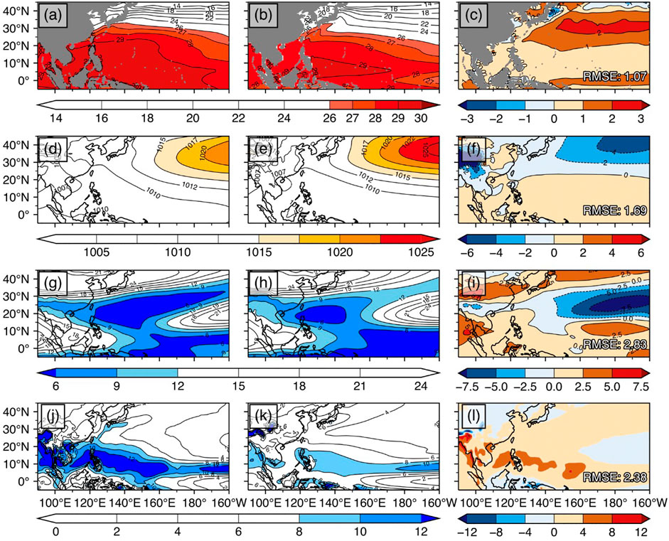
FIGURE 1. June-to-October mean sea surface temperature (°C) for the period of 1979–2005, derived from (A) JRA-55 and (B) CESM. (C) is the difference between (A) and (B). (D–F), (G–I), (J–L) show means of the same period but for sea level pressure (hPa), zonal wind shear (m/s), and total precipitation rate (mm/day), respectively.
Pressure is high over the central part of the North Pacific (Figures 1D,E), while pressure on the Asian continent and low-latitude ocean surface is relatively low. There is higher pressure over central Pacific in CESM, with the 1,015 hPa isobaric line extending to 150°E. Nonetheless, the pressure patterns are very similar between the two datasets.
There are two minima in the wind shear (defined as the absolute value of the difference between zonal winds at 200 hPa and 850 hPa) field over the Northwest Pacific (Figures 1G,H); one is a band over the low-latitudes of central and western Pacific, while the other is an area east of Taiwan and the Philippines. The area of minimum wind shear is larger in JRA-55, with 6 m s−1 contour extending to the central Pacific. Appropriate wind shear has an important effect on the generation and rapid intensification of TCs. The biases were potentially suggested that the total number and intensity of TCs from the model were underestimated compared to the reanalysis results.
The location and shape of the precipitation belts are relatively similar between the two datasets (Figures 1J,K), but the precipitation intensity is very different. Precipitation did not exceed 12 mm day−1 over the sea in CESM, and near-equatorial precipitation is less than 8 mm day−1 from 115 °E to 120 °E. Both features indicate that the water vapor in CESM is lower than the reality. The root mean square error (RMSE) (Anthes 1983; Lo et al., 2008) is often used to calculate the difference between model simulation and reality (the third column of Figure 1). The results showed that there are high consistencies between model results and reanalysis in terms of SST and SLP.
In summary, JRA-55 and CESM were compared during the same time period. Although CESM has lower SST and stronger wind shear compared to JRA-55, the shape of the Pacific Warm Pool, the locations of high pressure, and the locations of the minimum wind shear are in good agreement with JRA-55; CESM simulated credible climatological conditions (Figures 1C,F,I,L).
After extensive testing, we found that the combination of TMTN = 5 and LTMD = 56.67 km/h produced good accuracy in identifying TCs. Table 1 shows the comparison result between best track data and the results obtained by using the algorithm on JRA-55 and ERA5 in the various spatial resolutions. Most of the sensitivity [Hit/(Hit + Miss)] is over 80%, most of the false alarm rate [False Alarm/(False Alarm + Hit)] is below 25% and all tracking results have significant correlation coefficients, indicating good performance of the tracking algorithm when the spatial resolution is finer than 2.0° × 2.0°.
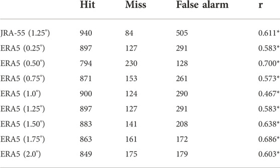
TABLE 1. Comparison between tracking result and JMA best track data. First three columns of data represent hit, miss and false alarm number of TCs. The last column of data is the correlation coefficient. An asterisk indicates that the data is significant with a significance level of 95%.
It was noted that a relatively high false rate induced by is the algorithm in the high resolution was related to the low correlation coefficient. The high false rate was indicated that there were many vortexes which were not real TCs in the recognition results. It was probably due to the interpolation method does not eliminate all the high frequency signals, and some non-TC systems with high relative vorticity were still left in the interpolated data. As a result, some of them were identified as TCs by the tracking algorithm.
3.2 Projection of west Pacific TC
3.2.1 Changes of background field
To understand TC changes in the 21st century, we will compare the background fields between the end (2091–2100) and the start (2011–2020) of this century. Figure 2 shows the difference in the background fields between the end and the beginning of the 21st century. SSTs increase by more than 0.8°C in the equatorial and low-latitude Pacific regions under the 2.0degNE scenario. Warm SSTs are conducive to the generation and development of TCs, and the main area of TC generation and development is located in the 30°C Pacific Warm Pool, hence the mean TC intensity under the 2.0degNE scenario may be higher than under other scenarios.
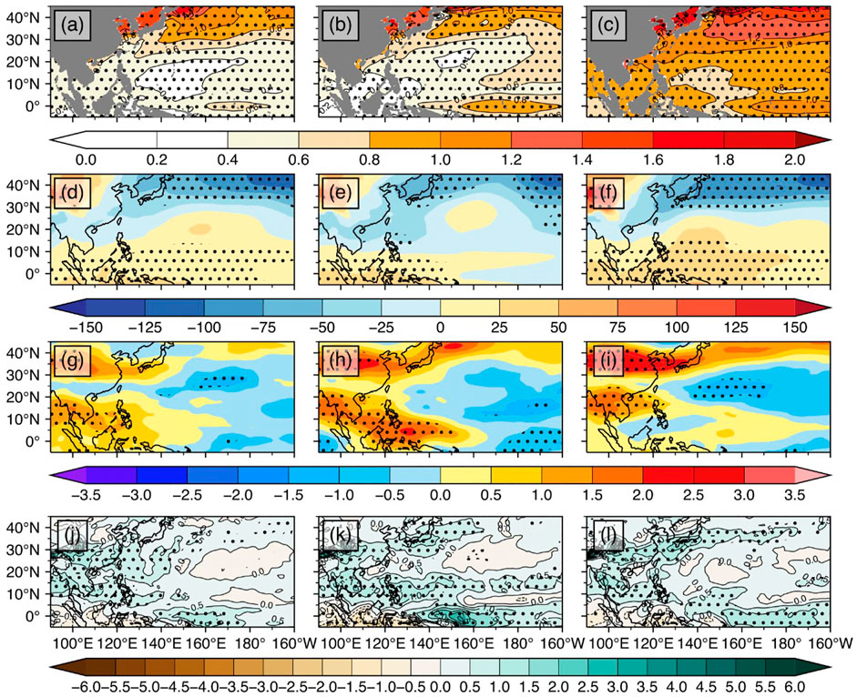
FIGURE 2. Changes of June-to-October monthly mean sea surface temperature (°C) in the end of 21st century, defined as the 2011–2020 mean subtracted from the 2091–2100 mean, under the (A) 1.5degNE, (B) 1.5degOS, and (C) 2.0degNE scenarios. (D–F), (G–I), (J–L) show similar calculations but for sea level pressure (hPa), zonal wind shear (m/s), and total precipitation rate (mm/day), respectively. The area covered by the points passed the 95% significance test.
As the magnitude of global warming increases, the range and amplitude of high sea level pressure regions over northwest China and the low latitudes increases, while the low SLP regions over the mid-latitudes gradually extend to Japan and the coastal areas of China. This shows that global warming may strengthen the high- and low-pressure systems. The low SLP field along the coast may promote TC intensification before landfall.
The reductions in range and magnitude of wind shear over the midwestern North Pacific are greater under the 1.5degOS and 2.0degNE scenarios. As the magnitude of global warming increases, the areas of dense TC generation and rapid intensification may move more eastward, hence TCs have more time to develop before landfall and the mean TC intensity at landfall increases.
Changes in precipitation rate show a trend consistent with global warming. Under the 2.0degNE scenario, the mid-latitude rain belt extends to the central North Pacific, while the drier area in the subtropical zone shrinks. Hence more places experience increase than decrease of precipitation.
3.2.2 Changes of the numbers of TC and PDI
We performed linear regression on data from different ensemble members and plotted the 9-year moving mean of the number of TCs. The result is shown in Figures 3, 4. Due to the coarse spatial resolution of the model, the absolute numbers of TCs are not comparable with reality. The interannual fluctuations of TCs under different scenarios are very large. Regression analysis shows that the number of TCs under each scenario increases with time, and the number of TCs in the 1.5degNE, 1.5degOS and 2.0degNE increased by 0.43, 0.59, 0.19 in 95 years, respectively. The mean number of TCs over 95 years is about 0.1 higher under the 1.5degNE and 1.5degOS scenarios compared to the 2.0degNE scenario. It is noted that the results of 1.5degOS scenario passed the 95% significance test.
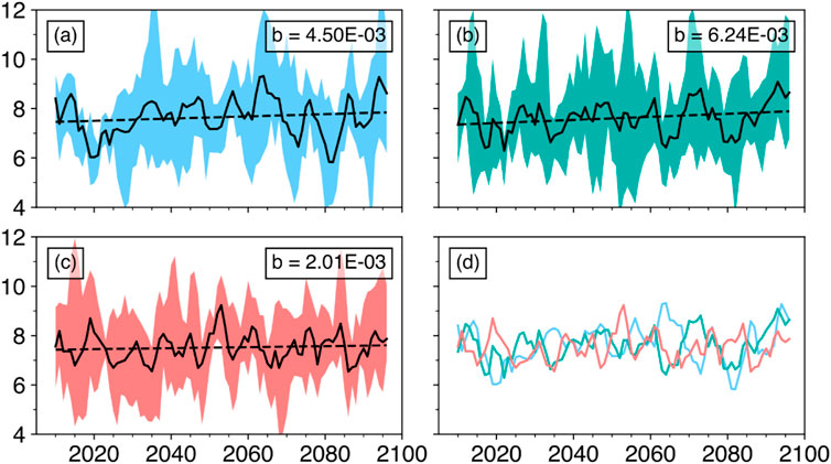
FIGURE 3. Annual numbers of tropical cyclones identified by the algorithm from simulations under the (A) 1.5degNE, (B) 1.5degOS, and (C) 2.0degNE scenarios. 9-Year moving means are taken from 2006 to 2100. The shaded area represents the ensemble range, the black solid line the ensemble mean, and the black dotted line result of linear regression. (D) Ensemble means of the annual number of tropical cyclones from averaged values in the 1.5degNE (blue), 1.5degOS (green), and 2.0degNE (red) scenarios.
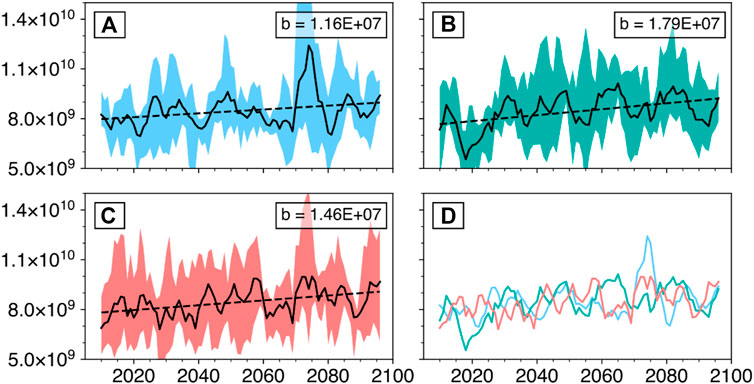
FIGURE 4. The annual mean Power Dissipation Index (PDI) of tropical cyclones from 2006 to 2100, calculated from simulations under (A) 1.5degNE, (B) 1.5degOS, (C) 2.0degNE scenarios. The shaded area represents the ensemble range, the black solid line the ensemble mean, and the black dotted line the result of linear regression. (D) Ensemble means of the annual mean (PDI) in the 1.5degNE (blue), 1.5degOS (green), 2.0degNE (red) scenarios.
The power dissipation index (PDI) increases under the three scenarios (Figure 4), the maximum is under the 1.5degOS scenario. The increase in 2.0degNE scenario is slightly less than that of the1.5degOS. At the end of the 21st century, the maximum averaged PDI is under the 2.0degNE scenario and the minimum is under the 1.5degOS scenario. The results in all scenarios passed the 95% significance test.
It is concluded that the annual number of TCs may not have a significant growth under the 1.5degNE and 2.0degNE scenarios, however, the mean energy of a single TC will increase significantly, and the potentially destructive impact of each TC may be greater.
3.2.3 Changes of TC paths
We use a TC activity frequency chart to evaluate the changes to TC paths over time. Due to the limited and discrete cyclone location points in TC path data, we consider the entire area covered by each TC. This is a clump of grid-points near the path grid-point, and is extracted by our algorithm. The frequency of TC activity at these grid-points is calculated as follows:
Assuming that the discretized center of a TC is located at a certain time on the grid-point with indices (m, n), then the activity frequency at this grid point is defined to be 1, the activity frequency at the 4 grid-points directly adjacent to (m, n) is defined to be 1/2, the activity frequency at the 4 grid-points diagonally adjacent to (m, n) is defined to be
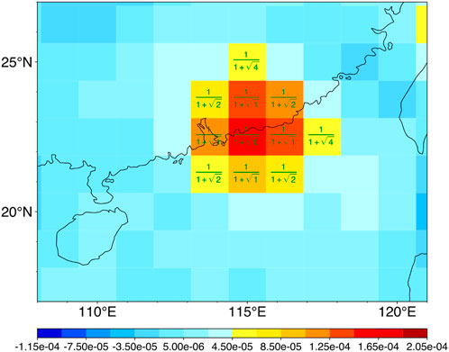
FIGURE 5. Relative vorticity field at 1979-7-29 12:00 UTC. The yellow and red grids in the center of the figure indicate the scope of the vortex. The green numbers indicate TC activity frequencies.
The TC activity frequency plot described above is totally different from the TC tracking density plot. The TC tracking density generally defined as “individual TCs entering or forming within a grid box” (Bell et al., 2019a; Bell et al., 2019b), which only considers one grid point for each typhoon in one time. The method in this study considers the size of TCs, so the plots more realistically depict the impact in different regions.
The 10-year accumulated activity at the beginning and end of the 21st century is shown in Figure 6. Regardless of the time period, the southern part of the South China Sea and the Pacific Ocean to the east of the Philippines are the areas of dense TC track. At the end of the 21st century, the frequency of TC occurrence is higher in the low latitudes closer to the equatorial Pacific Ocean than at the beginning of the 21st century. Under the 1.5degNE and the 2.0degNE scenarios, more TCs move northeast instead of moving west to make landing on the southeast China. Dense landing areas are not found in northern China or Japan in these two scenarios, but the number of TCs landing in northern China significantly increases, especially under the 2.0degNE scenario.
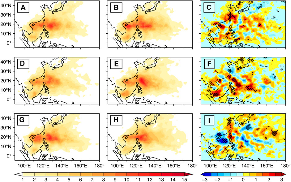
FIGURE 6. 10-year accumulated activity frequency of tropical cyclones in the 1.5degNE scenario, for the periods of (A) 2011–2020 and (B) 2091–2,100. (C) is the difference between (A) and (B). (D–F), (G–I) show the same variable for the 1.5degOS and 2.0degNE scenarios, respectively. The area that passed the 95% significance test is covered by the meshes.
4 Conclusion and discussion
CESM simulations from the Community Earth System Model Large Ensemble Project and limited warming simulations (Sanderson et al., 2017) were evaluated in terms of climatological background fields and changes to TC activity in the Northwest Pacific over the past 35 years and the next 95 years.
(1) Under the three temperature rise targets (1.5degNE, 1.5degOS, 2.0degNE), there are certain changes to the background fields. The sign of the changes is the same in theory, but under all scenarios, the increases in sea surface temperature and precipitation rate are not as high as that simulated by other GCMs.
(2) The model data shows that the number of TCs in the 21st century shows a fluctuating upward trend (0.43, 0.59, 0.19 in 95 years under 1.5degNE, 1.5degOS, and 2.0degNE, respectively). The annual number of TCs and the average PDI increases faster over time under the 1.5degOS scenario. Therefore, the total energy of TCs is greater and the impact on human society is greater.
(3) The changes to TC paths common to all three scenarios are as follows: Near 5°N in the South China Sea is an area where TCs are frequently occur; The major paths of TCs generated in the Northwest Pacific are: 1) Pass between Taiwan and the Philippines then landing on Hainan Island; 2) Landing on Taiwan Island or the Yangtze River Delta region. There are slight differences in major TC paths between different scenarios. In the 1.5degNE and 2.0degNE scenarios, TCs tend to turn to the east of Taiwan Island rather than land on mainland China.
Our TC identification algorithm shows good performance, but there are situations where it fails. This problem can be solved by changing the algorithm’s threshold parameters. Although all datasets were interpolated to the same spatial resolution, there may still be slight differences in the optimal parameters for different data.
The time spent in the data preprocessing stage (the interpolation) of our tracking algorithm accounts for a considerable part of total running time, which also requires large memory space. This problem may be solved by using artificial neural networks (ANNs) which is a kind of the machine learning model. As mentioned in Section 2.2.2, there is a clear difference between the shape of vortex (round or spiral) and the shape of noise (banded). Figure 7 shows part of the relative vorticity fields of TCs and noise captured from ERA5. ANNs may easily learn these two features and produce a better result, while significantly speeding up the tracking process and reducing the memory requirement.
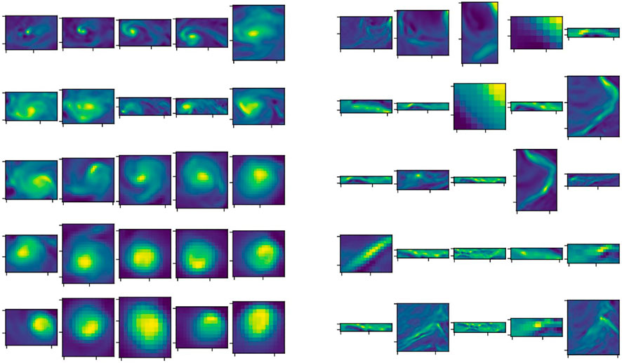
FIGURE 7. Some relative vorticity fields of TCs (left) and noise (right), which was captured during running the tracking algorithm.
This study is based on the ensemble members of a single model. The conclusion obtained will have biases, but the algorithm can be used with other model data. We believe the results obtained after using this algorithm on multiple models will be closer to reality.
Data availability statement
All the data in this study are publicly available and cited in the references. GPCP precipitation data at https://psl.noaa.gov/data/gridded/data.gpcp.html. NOAA Extended Reconstructed Sea Surface Temperature (SST) V5 at https://psl.noaa.gov/data/gridded/data.noaa.ersst.v5.html. CESM large ensemble historical experiment data set can be downloaded at http://www.cesm.ucar.edu/projects/community-projects/LENS/data-sets.html. CESM low warming simulations data set can be found at https://doi.org/10.5065/D6RV0MD6. JMA best track data can be downloaded at https://www.jma.go.jp/jma/jma-eng/jma-center/rsmc-hp-pub-eg/besttrack.html. CMA best track data at http://tcdata.typhoon.org.cn/zjljsjj_sm.html. JRA55 reanalysis can be found at https://jra.kishou.go.jp/JRA-55/index_en.html. ERA5 reanalysis can be found at https://cds.climate.copernicus.eu/#!/search?text=era5.
Author contributions
ZJ contributed to conception and design of the study. HD programmed the algorithm. HD and XZ organized the database. HD and ZJ performed the statistical analysis. ZJ and HD wrote the first draft of the manuscript. All authors contributed to manuscript revision, read, and approved the submitted version.
Funding
This study was funded by the National Natural Science Foundation of China (Grants Nos. U1811464 and U21A6001), the Guangdong Major Project of Basic and Applied Basic Research (2020B0301030004), and the Innovation Group Project of Southern Marine Science and Engineering Guangdong Laboratory (Zhuhai) (No. 311020008).
Conflict of interest
The authors declare that the research was conducted in the absence of any commercial or financial relationships that could be construed as a potential conflict of interest.
Publisher’s note
All claims expressed in this article are solely those of the authors and do not necessarily represent those of their affiliated organizations, or those of the publisher, the editors and the reviewers. Any product that may be evaluated in this article, or claim that may be made by its manufacturer, is not guaranteed or endorsed by the publisher.
Supplementary material
The Supplementary Material for this article can be found online at: https://www.frontiersin.org/articles/10.3389/fenvs.2022.1046890/full#supplementary-material
References
Anthes, R. A. (1983). Regional models of the atmosphere in middle latitudes. Mon. Weather Rev. 111, 1306–1335. doi:10.1175/1520-0493
Bell, G. D., and Bosart, L. F. (1989). A 15-year climatology of Northern Hemisphere 500 mb closed cyclone and anticyclone centers. Mon. Weather Rev. 117, 2142–2164. doi:10.1175/1520-0493
Bell, S. S., Chand, S. S., Camargo, S. J., Tory, K. J., Turville, C., and Ye, H. (2019b). Western North Pacific tropical cyclone tracks in CMIP5 models: Statistical assessment using a model-independent detection and tracking scheme. J. Clim. 32, 7191–7208. doi:10.1175/jcli-d-18-0785.1
Bell, S. S., Chand, S. S., Tory, K. J., Dowdy, A. J., Turville, C., and Ye, H. (2019). Projections of southern hemisphere tropical cyclone track density using CMIP5 models. Clim. Dyn. 52, 6065–6079. doi:10.1007/s00382-018-4497-4
Bell, S. S., Chand, S. S., Tory, K. J., and Turville, C. (2018). Statistical assessment of the OWZ tropical cyclone tracking scheme in ERA-Interim. J. Clim. 31, 2217–2232. doi:10.1175/jcli-d-17-0548.1
Blender, R., Fraedrich, K., and Lunkeit, F. (1997). Identification of cyclone-track regimes in the North Atlantic. Q. J. R. Meteorol. Soc. 123, 727–741. doi:10.1002/qj.49712353910
Blender, R., and Schubert, M. (2000). Cyclone tracking in different spatial and temporal resolutions. Mon. Weather Rev. 128, 377–384. doi:10.1175/1520-0493(2000)128<0377:ctidsa>2.0.co;2
Bluestein, H. B. (1992). Synoptic-dynamic meteorology in midlatitudes: Observations and theory of weather systems. Taylor & Francis.
Camargo, S. J., and Zebiak, S. E. (2002). Improving the detection and tracking of tropical cyclones in atmospheric general circulation models. Weather Forecast. 17, 1152–1162. doi:10.1175/1520-0434(2002)017
Chan, C. L., Johnny, S., and Sik, K. (2001). Improvements in the seasonal forecasting of tropical cyclone activity over the western North pacific. Weather Forecast. 16, 491–498. doi:10.1175/1520-0434(2001)016
Chan, J. C., and Liu, K. S. (2004). Global warming and Western North Pacific typhoon activity from an observational perspective. J. Clim. 17, 4590–4602. doi:10.1175/3240.1
Chauvin, F., Royer, J.-F., and Déqué, M. (2006). Response of hurricane-type vortices to global warming as simulated by ARPEGE-Climat at high resolution. Clim. Dyn. 27, 377–399. doi:10.1007/s00382-006-0135-7
Emanuel, K. (2005). Increasing destructiveness of tropical cyclones over the past 30 years. Nature 436, 686–688. doi:10.1038/nature03906
Fan, K. (2007). New predictor and new prediction model of typhoon frequency in the northwest pacific. Sci. CHINA Earth Sci. 37, 1260–1266. doi:10.1007/s11430-007-0105-x
Gao, X. J., Lin, Y. H., Zhao, Z. C., and Giorgi, F. (2003). Impacts of greenhouse effect on typhoon over China as simulated by a regional climate model. J. Trop. Oceanogr. 22, 77–83.
Haarsma, R. J., Roberts, M. J., Vidale, P. L., Senior, C. A., Bellucci, A., Bao, Q., et al. (2016). High resolution model Intercomparison project (HighResMIP v1.0) for CMIP6. Geosci. Model Dev. 9, 4185–4208. doi:10.5194/gmd-9-4185-2016
Hersbach, H., Bell, B., Berrisford, P., Hirahara, S., Horanyi, A., Munoz-Sabater, J., et al. (2020). The ERA5 global reanalysis. Q. J. R. Meteorol. Soc. 146, 1999–2049. doi:10.1002/qj.3803
Kay, J. E., Deser, C., Phillips, A., Mai, A., Hannay, C., Strand, G., et al. (2015). The community Earth system model (CESM) large ensemble project: A community resource for studying climate change in the presence of internal climate variability. Bull. Am. Meteorological Soc. 96, 1333–1349. doi:10.1175/bams-d-13-00255.1
Knutson, T., Camargo, S. J., Chan, J. C. L., Emanuel, K., Ho, C. H., Kossin, J., et al. (2020). Tropical cyclones and climate change assessment: Part II: Projected response to anthropogenic warming. Bull. Am. Meteorological Soc. 101, E303–E322. doi:10.1175/bams-d-18-0194.1
Knutson, T. R., Sirutis, J. J., Garner, S. T., Vecchi, G. A., and Held, I. M. (2008). Simulated reduction in Atlantic hurricane frequency under twenty-first-century warming conditions. Nat. Geosci. 1, 359–364. doi:10.1038/ngeo202
Kobayashi, S., Ota, Y., Harada, Y., Ebita, A., Moriya, M., Onoda, H., et al. (2015). The JRA-55 reanalysis: General specifications and basic characteristics. J. Meteorological Soc. Jpn. 93, 5–48. doi:10.2151/jmsj.2015-001
Lang, X., and Wang, H. (2008). Can the climate background of Western North Pacific typhoon activity be predicted by climate model? Sci. Bull. (Beijing). 53, 2392–2399. doi:10.1007/s11434-008-0266-9
Li, Q., Zhang, R., Yao, X. F., Ge, S. S., and Zou, H. W. (2013). Risk assessment and regionalization of tropical cyclone disaster over China's surrounding sea. J. Trop. Meteorology 29, 143–148.
Lo, J. C. F., Yang, Z. L., and Pielke, R. A., (2008). Assessment of three dynamical climate downscaling methods using the Weather Research and Forecasting (WRF) model. J. Geophys. Res. 113, D09112. doi:10.1029/2007jd009216
Nguyen, K., and Walsh, K. (2001). Interannual, decadal, and transient greenhouse simulation of tropical cyclone–like vortices in a regional climate model of the South Pacific. J. Clim. 14, 3043–3054. doi:10.1175/1520-0442(2001)014
Sanderson, B. M., Xu, Y., Tebaldi, C., Wehner, M., O'Neill, B., Jahn, A., et al. (2017). Community climate simulations to assess avoided impacts in 1.5 and 2 C futures. Earth Syst. Dyn. 8, 827–847. doi:10.5194/esd-8-827-2017
Su, Z. Z., Yu, J. H., Sun, C. H., Ren, F. M., Wang, Y. Q., and Liang, X. Y. (2010). The initial evaluation of tropical cyclone potentialpredictability in the northwestern pacific using the iprc regional climate model. J. Trop. Meteorology 26, 165–173.
Tory, K. J., Dare, R., Davidson, N., McBride, J., and Chand, S. (2013). The importance of low-deformation vorticity in tropical cyclone formation. Atmos. Chem. Phys. 13, 2115–2132. doi:10.5194/acp-13-2115-2013
Vecchi, G. A., and Soden, B. J. (2007). Increased tropical Atlantic wind shear in model projections of global warming. Geophys. Res. Lett. 34. doi:10.1029/2006gl028905
Wang, H. J., Fan, K., Sun, J. Q., Lang, X. M., and Lin, M. J. (2007). Some advances in the researches of the western North pacific typhoon climate variability and prediction. Chin. J. Atmos. Sci. 31, 1076–1081.
Wang, H. J., Lang, X. M., Fan, K., Sun, J. Q., and Zhou, G. Q. (2006). Real-time climate prediction experiment for the typhoon frequency in the western North pacific for 2006. Clim. Environ. Res. 11, 133–137.
Webster, P. J., Holland, G. J., Curry, J. A., and Chang, H.-R. (2005). Changes in tropical cyclone number, duration, and intensity in a warming environment. Science 309, 1844–1846. doi:10.1126/science.1116448
Wu, J., Gao, X.-J., Zhu, Y. M., Shi, Y., and Giorgi, F. (2022). Projection of the future changes in tropical cyclone activity affecting East Asia over the Western North Pacific based on multi-RegCM4 simulations. Adv. Atmos. Sci. 39 (2), 284–303. doi:10.1007/s00376-021-0286-9
Wu, W., and Yu, J. H. (2011). Scenarios of 21st century tropical cyclone activity over western North pacific as projected by GFDL_RegCM. J. Trop. Meteorology 27, 843–852.
Ying, M., Knutson, T. R., Kamahori, H., and Lee, T. C. (2012). Impacts of climate change on tropical cyclones in the western North pacific basin. Part II: Late twenty-first century projections. Trop. Cyclone Res. Rev. 1, 291–295.
Zhang, C. Y., Feng, Z. G., Zhang, X. K., and Zhang, Q. L. (2017). Analysis on research progress of Kuroshio. WORLD SCI-TECH R&D 39, 239–249.
Zhang, J. Y., Wu, L. G., and Zhang, Q. (2011). Tropical cyclone damages in China under the background of global warming. J. Trop. Meteorology 27, 442–454.
Zhang, Y., and Wang, H. J. (2010). A projection of future climate change over the western North pacific related to typhoon activities. Acta Meteorol. Sin. 68, 539–549.
Keywords: tropical cyclone, detecting and tracking, projection, climate change, algorithm
Citation: Deng H, Ji Z, Zhu X and Dong W (2022) Future changes of tropical cyclone activity over the west Pacific under the 1.5°C and 2°C limited warming scenarios using a detecting and tracking algorithm. Front. Environ. Sci. 10:1046890. doi: 10.3389/fenvs.2022.1046890
Received: 17 September 2022; Accepted: 03 November 2022;
Published: 18 November 2022.
Edited by:
Haipeng Yu, Northwest Institute of Eco-Environment and Resources (CAS), ChinaReviewed by:
Xuejie Gao, Institute of Atmospheric Physics (CAS), ChinaDaoyi Gong, Beijing Normal University, China
Jianping Tang, Nanjing University, China
Copyright © 2022 Deng, Ji, Zhu and Dong. This is an open-access article distributed under the terms of the Creative Commons Attribution License (CC BY). The use, distribution or reproduction in other forums is permitted, provided the original author(s) and the copyright owner(s) are credited and that the original publication in this journal is cited, in accordance with accepted academic practice. No use, distribution or reproduction is permitted which does not comply with these terms.
*Correspondence: Zhenming Ji, aml6aG0zQG1haWwuc3lzdS5lZHUuY24=