High-resolution 3D mapping of cold-water coral reefs using machine learning

Structure-from-Motion (SfM) photogrammetry is a time and cost-effective method for high-resolution 3D mapping of cold-water corals (CWC) reefs and deep-water environments. The accurate classification and analysis of marine habitats in 3D provide valuable information for the development of management strategies for large areas at various spatial and temporal scales. Given the amount of data derived from SfM data sources such as Remotely-Operated Vehicles (ROV), there is an increasing need to advance towards automatic and semiautomatic classification approaches. However, the lack of training data, benchmark datasets for CWC environments and processing resources are a bottleneck for the development of classification frameworks. In this study, machine learning (ML) methods and SfM-derived 3D data were combined to develop a novel multiclass classification workflow for CWC reefs in deep-water environments. The Piddington Mound area, southwest of Ireland, was selected for 3D reconstruction from high-definition video data acquired with an ROV. Six ML algorithms, namely: Support Vector Machines, Random Forests, Gradient Boosting Trees, k-Nearest Neighbours, Logistic Regression and Multilayer Perceptron, were trained in two datasets of different sizes (1,000 samples and 10,000 samples) in order to evaluate accuracy variation between approaches in relation to the number of samples. The Piddington Mound was classified into four classes: live coral framework, dead coral framework, coral rubble and sediment and dropstones. Parameter optimisation was performed with grid search and cross-validation. Run times were measured to evaluate the trade-off between processing time and accuracy. In total, eighteen variations of ML algorithms were created and tested. The results show that four algorithms yielded f1-scores >90% and were able to discern between the four classes, especially those with usually similar characteristics, e.g., coral rubble and dead coral. The accuracy variation among them was 3.6% which suggests that they can be used interchangeably depending on the classification task. Furthermore, results on sample size variations show that certain algorithms benefit more from larger datasets whilst others showed discrete accuracy variations (<5%) when trained in datasets of different sizes.

1 Introduction

Cold-water corals (CWC) play an important role in deep-sea ecosystems (Rogers 1999; Costello et al., 2005). Species such as Lophelia pertusa (synonymized to Desmophyllum pertusum (Addamo et al., 2016) and Madrepora oculata are formed by three-dimensional (3D) calcareous frameworks that can baffle bypassing sediments (Dorschel 2003; Titschack et al., 2015; Lim et al., 2020a), and given favourable environmental conditions (e.g., hydrodynamic regime, temperature and nutrient supply), they can form positive topographic features such as coral patches, mounds, reefs and giant carbonate mounds (Mortensen et al., 1995; Freiwald, 2002; Wheeler et al., 2005a; Freiwald and Roberts, 2005; Wheeler et al., 2007; Guinan et al., 2009; Roberts et al., 2009; Lim et al., 2017; 2020b). CWC reefs are associated with highly diverse faunal assemblages (Rogers 1999) being often considered “biodiversity hotspots” of deep-sea environments (Turley, Roberts, and Guinotte 2007; Lim et al., 2018a; Boolukos et al., 2019; Dorey et al., 2020) as they act as a refuge and nursery for deep-sea species, including commercial fish (Fosså, Mortensen, and Furevik 2002; Turley, Roberts, and Guinotte 2007). The association of not only live coral frameworks but also dead corals and coral rubbles is also considered key for the development of microhabitats that promote enhanced biodiversity (Luckhurst and Luckhurst 1978; Buhl-Mortensen et al., 2010; Henry and Murray Roberts 2017; Lim et al., 2020b; Clippele et al., 2021). However, these vital ecosystems are impacted by anthropogenic activities such as bottom trawling, deep sea mining and oil and gas exploration (Rogers, 1999; Wheeler et al., 2005a; Turley et al., 2007; Boolukos et al., 2019). Studies evidence the impact of fishery-related activities and climate change in CWCs, suggesting that coral health is affected by trawling and/or dredging (Rogers, 1999; Roberts et al., 2000; Wheeler et al., 2005b; Althaus et al., 2009), ocean acidification, CO₂ emission and ocean uptake leading to a decrease of ocean pH (Turley, Roberts, and Guinotte 2007) and rising temperatures (Gori et al., 2016).

As 3D structures, CWCs enhance small scale spatial variability and influence species biodiversity and nutrient cycling (Graham and Nash 2013; Pizarro et al., 2017; Lim et al., 2018b). However, the analysis of these environments often rely on planar derivatives from 1D or 2D estimates of coral reef coverage, rugosity and distribution that may disregard key variations on coral habitats, as accurate vertical and volumetric information may not be integrated into the analysis (Cocito et al., 2003; Courtney et al., 2007; Goatley and Bellwood 2011; House et al., 2018). Whilst 2D approaches are useful to produce rapid estimates of coral reef health (Kornder et al., 2021), they may overlook the naturally complex 3D morphology of corals reefs and maximise the tendency of large coral colonies to obscuring understory biota (Goatley and Bellwood 2011; Bergh et al., 2021; Kornder et al., 2021) represented by the so-called ‘canopy’ effect. Therefore, there is a demand for novel mapping methods that will take into account the 3D morphological structure of CWC in order to better understand the key drivers and controls of CWC environments.

Structure from Motion (SfM) is a relatively new branch of photogrammetry that can be applied to geospatially reconstruct seabed habitats whilst providing detailed descriptors regarding coral reef conditions and microhabitats (Ferrari et al., 2017; Pizarro et al., 2017; Conti, Lim, and Wheeler 2019; Price et al., 2019, 2021; Calders et al., 2020; Lim et al., 2020c; Urbina-barreto et al., 2021; Urbina-Barreto et al., 2022). In contrast to traditional photogrammetry, SfM uses algorithms such as Scale Invariant Feature Transform (SIFT) (Lowe 1999) to identify matching features in a set of overlapping images whilst calculating the variations in camera orientation and position of the matched features (Carrivick, Smith, and Quincey 2016). The process yields high-resolution 3D reconstructions of different landscapes in the form of 3D point clouds, meshes, digital elevation models (DEMs) and orthomosaics (geometrically-corrected, scaled and georeferenced mosaic of images containing RBG information) (Carrivick, Smith, and Quincey 2016). Besides requiring less time and cost resources when compared to traditional seabed mapping techniques such as the ‘chain-and-tape’ method (Storlazzi et al., 2016), SfM and 3D photogrammetry enables non-destructive quantitative monitoring of: 1) biological estimates, e.g., benthic cover, coral colony health, abundance and size (Burns J. H. R. et al., 2015; Lange and Perry 2020; Pascoe et al., 2021); 2) physical estimates of reef terrain features such as slope, fractal dimension, surface and structural complexity (Burns D. et al., 2015; Figueira et al., 2015; Leon et al., 2015; Storlazzi et al., 2016; Fukunaga and Burns 2020; Urbina-barreto et al., 2021) up to very high-resolution analysis at colony scale such as 3) sub-centimetre reconstructions of individual branches and polyps (Cocito et al., 2003; Gutierrez-Heredia et al., 2016; Lange and Perry 2020).

The application of computer vision and machine learning (ML) methods in remote sensing has contributed to unprecedented progress in automated spatial (Gilardi 1995; Pal 2005; Mountrakis et al., 2011; Belgiu and Drăgu 2016; Durden et al., 2021) and marine data analyses (Beijbom et al., 2012; Beijbom et al., 2015; Williams et al., 2019; Summers, Lim, and Wheeler 2021). The use of supervised and unsupervised ML classification methods has rapidly grown, especially in the context of underwater image analysis (Huang, Brooke, and Harris 2011; Shihavuddin et al., 2013; Young 2018; Conti, Lim, and Wheeler 2019; Yu et al., 2019; Lim et al., 2020c; González-Rivero et al., 2020). Advancements have been made with the application of assembled ML algorithms and deep-learning such as convolutional neural networks (CNNs) to automate the annotation process by applying path-based image classification techniques to assign labels automatically to unseen images (Shihavuddin et al., 2013; Modasshir et al., 2018; Mahmood et al., 2019) and alternatively using the classified images to produce 3D models (Mohamed, Nadaoka, and Nakamura 2020). Recent studies used CNNs such as ResNET152 to generate dense labels from sparse label annotation by extracting patches of the 3D models (Hopkinson et al., 2020). Other studies have created a combined approach by using CNN for sparse label annotation through patch extraction and using the resulting classified images to produce 3D models of the environment (Pierce et al., 2021).

Point clouds are composed by a set of points containing coordinates (X, Y, Z) oriented in a cartographic space. 3D models derived from point clouds are useful to optimise the trade-off between precision and geometric complexity (Poux et al., 2018). However, the semantic segmentation of point clouds, while having numerous real word applications, has been considered a challenge (Poux et al., 2018; Xu et al., 2018; Yuval et al., 2021). Deep learning has advanced in favour of image segmentation and classification tasks, but its use towards semantic point cloud segmentation needs to be further explored (Karara, Hajji, and Poux 2021). Representation models such as PointNET which learn features directly from unstructured point data, i.e., dense clouds/point clouds are considered state-of-the-art techniques for dense cloud classification (Qi et al., 2017). However, these frameworks require large annotated datasets and computational requirements for producing meaningful results (Gilardi 1995; Yuval et al., 2021). In the context of deep-water environments, the lack of training data available has reportedly been the bottleneck for advances of ML algorithms (Roelfsema et al., 2021; Walker, Bennett, and Thornton 2021; Mohamed, Nadaoka, and Nakamura 2022). Although annotation frameworks to gather specific data from underwater environments have been developed (Beijbom et al., 2012; Beijbom et al., 2015; Zurowietz et al., 2018), there is still a need for specifically designed dataset benchmarks for the application of robust ML methods for 3D points clouds of deep-water environments. Additionally, researchers are continuously working towards minimising the effects of the “black box issue” to properly understand the machine decision process in the classification and how parameters and data affect the output (Gilardi 1995; Castelvecchi 2016).

In this study, we intend to tackle the automatic classification problem with a different approach. Instead of classifying the images to produce the 3D models, we created a classification framework to classify the 3D models directly, minimizing the need to provide extensive manual image annotations. As of this moment, this study is the first of the field to provide a comparison and performance analyses of six ML algorithms applied in 3D point clouds of CWC reefs. A number of studies have performed comparison analyses using widely used ML algorithms such as Support Vector Machines (SVMs), Neural Networks (NNs) and common ensemble methods, e.g., Random Forests (RFs) and Gradient Boosting Trees (GBTs) in multispectral imagery (Dixon and Candade 2008; Liu et al., 2017; Zhang et al., 2017; Fu et al., 2018; Jodzani, Johnson, and Chen 2019). Although insightful contributions can be drawn from such analyses, these studies focused on land use and classification of urban areas. Therefore, the fundamental properties of these algorithms for marine mapping applications are not well understood and advancements are required in order to progress on seabed habitat mapping of larger areas. To this end, this research bridges the knowledge gap between ML and CWC classification in 3D by providing a comparison of ML algorithms, performance analyses whilst delivering an optimised workflow the for classification of photogrammetry derived data.

This study applies ML classification to 3D photogrammetric reconstructions of coral reef habitats to analyse the outputs, data requirements and constraints of the coupled application of both methods. We aim to develop a novel classification method using SVM, RF, k-Nearest Neighbours (kNN), Logistic Regression (LR), GBT and Multilayer Perceptron (MLP) algorithms. Furthermore, this paper presents the results of an empirical comparison of seven supervised learning algorithms and evaluated by four performance criteria (f1 score, receiver operating characteristic (ROC) curves, area under the curve (AUC) scores and f1 scores of k-fold cross-validations). Each algorithm was analysed based on: 1) its suitability to the given classification task 2) their hyperparameters and processing times, and; 3) its performance with two datasets of different sample sizes (1,000 and 10,000 samples) to analyse the trade-off between accuracy, processing times and sample size.

2 Study area

The Piddington Mound is a CWC mound located in the Belgica Mound Province (BMP), Porcupine Seabight, NE Atlantic. The mound was selected to develop this study given the existence of high-definition (HD) video data and bathymetric surveys covering a large extent of the area (Lim et al., 2017), the evidence of temporal changes in coral cover (Boolukos et al., 2019) and dynamic sediment facies (Lim et al., 2018a; Conti, Lim, and Wheeler 2019). The BMP is a designated Special Area of Conservation (SAC) under the EU Habitats Directive located on the eastern margin of the Porcupine Seabight, southwest of Ireland (Figures 1A,B).

FIGURE 1

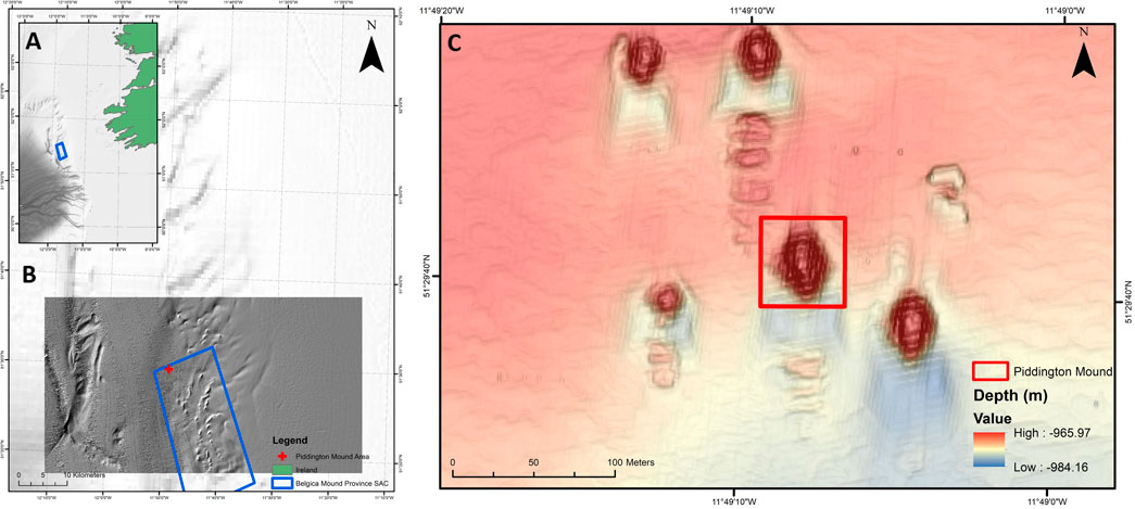
FIGURE 1. Map of the study site (A): Porcupine Seabight location relative to Ireland. The blue box indicates the location of the Belgica Mound Province (BMP) Special Area of Conservation (SAC) (B) Close view of the Porcupine Seabight and BMP with the Piddington Mound location indicated by the red cross (C) Bathymetric map of the Moira Mounds and location of the Piddington Mound Area (red box) within adjacent mounds.

The province hosts numerous CWC carbonate mounds and reefs dominated by framework-building scleractinian species Lophelia pertusa and Madrepora oculata (Huvenne et al., 2002; Wheeler et al., 2005b; Mol et al., 2007). Coral mounds in the BMP range from 3 to 10 m in height, e.g., the Moira Mounds (Wheeler et al., 2005b; Foubert et al., 2011; Wheeler et al., 2011), of which the Piddington Mound is one of the largest (Lim et al., 2017), to giant carbonate mounds that are up to 150 m high, e.g., the Challenger (Thierens et al., 2013), Therese Mound (Mol et al., 2007) and Galway Mound (Foubert et al., 2006; Dorschel et al., 2007). The Moira Mounds occur between 800 and 1,100 m water depth (Wheeler et al., 2005b) and have a semi-circular to ridge-shaped morphology with predominant alignment to the current direction (Wheeler et al., 2011). Comprising a small extent of 60 × 40 m in area (Foubert et al., 2006), the Moira Mounds are divided into a northern area, upslope area, midslope area and downslope area, where the Piddington Mound is located (Wheeler et al., 2011; Lim et al., 2018a). The Piddington Mound has documented current speeds of 40 cm s⁻¹ (Lim 2017). Previous work carried out by (Lim et al., 2017) have identified four distinct facies in the Piddington Mound area namely: live coral framework, dead coral framework, coral rubble and hemipelagic sediment with dropstones. These facies occur in a ring-like distribution, with coral rubble, live coral and dead coral frameworks distributed around the mound summit, forming an ‘on mound’ setting with high presence of corals, whilst sediments and drop stones occur where seabed becomes flat (Lim et al., 2017). These facies have also been adopted herein.

3 Materials and methods

This study is divided into a photogrammetry workflow to produce the 3D reconstructions of the Piddington Mound area and the development of multiclass classifications for these 3D point clouds. The photogrammetry process is outlined below followed by a description of the ML workflow. An overview of the classification algorithms, the model selection and the accuracy assessment is then further outlined. The ML workflow was executed in Python 3.8. Processing was executed with an Intel Core i7 CPU, 32 Gb RAM with NVIDIA Geforce RTX 2070 (8 Gb) graphics card (GPU). Here, the terms classification model, classifier and estimator are used interchangeably.

3.1 Photogrammetry

The data used in this study were acquired during the research cruise CE20011 (Lim et al., 2020b). The video data were collected with the ROV Holland 1 which is equipped with 11 camera systems. For this survey, two of these camera systems were used, namely: the HDTV camera (HD Insite mini-Zeus with HD SDI fibre output), and a Kongsberg OE 14–208 digital stills camera. The ROV is also mounted with two deep-sea lasers spaced at 10 cm for scaling. Positioning data were acquired with a Sonardyne Ranger 2 ultra-short baseline (USBL) beacon with accuracy of 1.3% of slant range (measurement of relative position from time of return signal from ROV transponder to the USBL in relation to the Turnaround Travel Time (TAT) and underwater sound velocity) similar to (Lim et al., 2020a; Oliveira et al., 2021). The ROV was kept at a height of approximately 2 m above the seabed with a survey speed of <0.2 knots during the video data collection. HD videos (1080p) were acquired at a rate of 50 frames per second (FPS) and stored as *.mov files. The section of the survey used herein was derived from one ROV dive performed as a grid with 35 lines spaced at 5 m from each other in a N-S direction. Previous seabed imaged acquisition studies showed that video mosaicking of a mound or grid of spaced lines yield more representative mosaics of CWC mounds (Lim et al., 2018a). In total, 4 h and 49 min of HD videos were recorded, summing 241.7 gigabytes (GB) of video data collected in one ROV dive.

The ROV video and navigation data were used to produce and georeference the 3D reconstructions. Video frames were extracted at a rate of 1 FPS from the raw video data with Blender (version 2.78). For the 3D point cloud reconstruction, frames were extracted and imported into Agisoft Metashape Professional version 1.7.2 (Agisoft-LLC 2020). Key point limit and tie point limits were chosen based on an empirical approach. Camera optimisation was performed after the camera alignment to refine the exterior and interior camera orientation parameters and triangulated tie point coordinates (Agisoft LLC, 2020). The dense point cloud was georeferenced with frame-relative USBL positioning data with X and Y coordinates, depth, yaw, pitch, roll and accuracy (°). The constant 10 cm distance from the parallel lasers of the ROV was used for scaling the model. The laser distance provides a measurement to scale and validate geometric uncertainties in the reconstruction process The site was separated into an on-mound and off-mound areas based on the depth difference between grid areas. The dense point cloud generated in the process was used for training and validation of the methodology.

A total of 7,301 images (1920 × 1,080 pixel resolution) were used in the point cloud reconstruction process. Camera optimization was applied using the focal length (f), radial distortion coefficients (K₁-K₃), and tangential distortion coefficients (P₁- P₂). The photo alignment process was performed with a key point limit of 20,000 and a tie point limit of 2,000. The yaw, pitch, roll and accuracy values were set to 135°, 0°, 0°, and 2 m, respectively.

3.2 Multiclass classification of 3D point clouds

3.2.1 Pre-processing

In this study, the point cloud created during the photogrammetry stage was used for the development of the ML workflow. The labelled dataset was created from the manual segmentation of point cloud objects into four classes. The classes were chosen to best represent the environmental variability of the specific area. The on-mound section of the Piddington Mound was chosen for reconstruction as it contained the largest volume of CWC and coral rubbles. The classes were outlined based on the analysis distribution of the regions of interest (ROIs), in this case, live coral framework (LCF), dead coral framework (DCF) and coral rubble (CR), apart from sediments and drop stones (SD).

Previous studies carried out in the Piddington Mound area have also adopted this classification scheme as it best represents the location (Lim et al., 2017). This potentially allows further comparisons over the temporal changes over the mound. A detailed class description was carried out for each class based on spatial distribution studies of the Piddington Mound and the Porcupine Bank Canyon (Lim et al., 2017; Appah et al., 2020). Table 1 provides a description of each class. The annotation process was performed in CloudCompare using the high-resolution orthomosaic as a visual aid.

TABLE 1

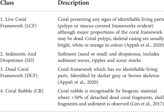
TABLE 1. Class label definitions used in the study.

The point cloud was composed of a set of points and their relative feature values. Each point contained information of 7 features (X, Y, Z, R, G, B and Normal_Y) and its ground truth label. Following the feature selection and labelling, the point cloud was separated into two datasets, namely dataset 1, composed of 1,000 samples and dataset 2, consisting of 10,000 samples. Each dataset was split into training and validation sets at a ratio of 75%/25%. In addition, a test set composed of 10,000 random samples was created from the points that remained from the initial point cloud after the train and test set were extracted. Therefore, the model evaluation was performed on the validation set and an additional cross-validation was performed on the test set.

After the training and testing splits were performed, datasets were scaled with a MinMax scaler, which was fitted on the training set of dataset 2 and applied to the remainder datasets (validation set of dataset 2 and training and validation sets of dataset 1). Synthetic Minority Oversampling Technique (SMOTE) (Chawla et al., 2002) was applied to balance the training set. SMOTE works by making a linear interpolation of a randomly selected observation from the minority class with another k-nearest neighbour of the same minority class. The new sample is created from the interpolation of those two samples. Previous studies have considered the oversampling approach to be beneficial for classification results in commonly used classifiers (Last, Douzas, and Bacao 2017) and CNNs (Buda, Maki, and Mazurowski 2018).

3.2.2 Classification algorithms

3.2.2.1 Random Forest

The RF algorithm is a tree-based ensemble classifier where each classifier is created using a random vector sampled from the input vector. Each tree provides a unit vote for the most popular class to classify the input vector (Pal 2005). Predictions are generated as an ensemble estimate from a number of decision trees from bootstrap samples (termed bagging) (Hengl et al., 2018). RF classifications have been successfully applied in a number of marine (Robert et al., 2016; Misiuk et al., 2019; Shang et al., 2021; Price et al., 2022) and terrestrial studies (Schratz et al., 2019). Comparison performance studies in land cover suggest that RF has provided the best performance in object-based classification tasks (Ma et al., 2017).

In this study, the grid search and cross-validation was performed to find the best number of estimators, i.e., number of trees, and the number of maximum features to be considered for the best split. The number of estimators was set with options of ranging from 10 to 1,000 and the number of features was set to a range of 1–7 for the first sets of RFs. The Scikit-learn options ‘auto’ and ‘log2’ were also considered. The best-performance RF model was selected based on the accuracy considering the permutation of the grid search parameters. The other parameters were set to the default of Scikit-learn class. The full list of parameters can be found on the Scikit-learn webpage. In the case of RFs, four classifiers were trained with four different options of parameter grids. Each of these four variations of RFs was trained with datasets 1 and 2, resulting in 8 trained RF models.

3.2.2.2 Gradient Boosting Trees

GBT is another popular ensemble method closely related to RFs. The method trains an ensemble of trees based on minimising the loss function i.e., the measure of fit between the actual data and the modelled data, in each interaction. Each tree is improved by attempting to minimise the error of the previous tree (Jodzani, Johnson, and Chen 2019). Boosting refers to combining these weak learners, i.e., single decision trees so that the following tree model corrects the errors of the previous one (Friedman 2001). The learning rate is also introduced to control the robustness of the classifier. Empirical studies have attested to the efficiency of GBTs over other supervised learning algorithms (Caruana and Niculescu-Mizil 2006). The decision trees in the GBT tend to be robust with respect to the addition of irrelevant features (Friedman 2001).

Here, the parameter grid defined to find the optimal GBT parameters with the grid search were: learning rate, number of estimators, the maximum depth of estimators and the subsample rate. The learning rate was set to options of 0.0001, 0.001, 0.01, 0.1, 1. The number of estimators was defined to 10, 50, 100, 500 and 1,000. The subsample rate was set to a range of 0.5, 0.7 and 1. Although the default subsampling value in Scikit-learn is set to 1, the range of values was expanded to include other two values, 0.7 and 0.5, which is the suggested value of subsampling according to Buitinck et al. (2013). It is noteworthy that, if subsampling is set to a value >1, the classifier changes to Stochastic Gradient Boosting (Buitinck et al., 2013). In this study, two GBT classifiers were trained with one set of parameter grids.

3.2.2.3 Support Vector Machines

The SVM concept is based on the construction of optimal hyperplanes in a high dimensional space between a proximal training sample and the separating hyperplane (Pedregosa et al., 2011). SVMs have a regularization parameter ‘C’ and gamma (γ) that allow the control of the decision function complexity and the level of influence of each sample towards it. The main advantages of the SVMs are the regularization parameter, which allows the user to control over-fitting, the kernel trick and the convex optimization problem (no local minima) (Liu et al., 2017). Other studies suggested that one advantage of SVMs is that the objective function is convex which reflects on a relatively straightforward solution for the optimization problem even though the training involves nonlinear optimization (Bishop 2006). Furthermore Bishop (2006), affirms that the number of basis functions in SVM models is usually much smaller than the number of training points. Although they increase with the size of the training set, it still has the capacity to be computationally faster than other classifiers. The choice of kernel is also an equally crucial parameter (Burges 1998) as it gives SVMs the capacity to insert the data into a higher-dimensional space, so that data that is not linearly separable in the original input space can be separable in a higher-dimensional one (Russell and Peter 2010). The use of radial basis function (RBF) kernel has been the most common choice in recent studies as it generally provides a good trade-off between time efficiency and accuracy (Jodzani, Johnson, and Chen 2019; Pedregosa et al., 2011; Friedman 2013). In this study, three options of kernels on the grid search parameters were: polynomial, sigmoid and RBF. The range of regularization ‘C’ and γ parameters were set to 0.1, 110,100, and 1,0.1,0.01,0.001 respectively.

3.2.2.4 Logistic Regression

LR, also known as logit regression or MaxEnt, is a parametric supervised classification algorithm based on general linear models. The concept behind LR is that the classifier takes a set of input variables and creates an estimate probability for the target variable. The parameter grid established for the LR grid search was defined by a choice of penalty parameters l1, l2, elasticnet, or none and regularization ‘C’ parameter values. The optimisation algorithm was set to the options of liblinear, sag, saga, lbfgs which are termed the solvers. Empirical studies suggest that the use of the solver depends on the amount of data available (Buitinck et al., 2013). In small datasets, for example, liblinear can be considered a good choice whereas saga and sag can be faster for large datasets. The latter is also considered a good choice for high-dimensional data. Furthermore, in multiclass problems, the multinomial loss can only be handled by the solvers saga, sag, lbfgs and newton-cg. The scaling is also important as the solvers saga and sag can only reach faster convergence on features with proximal scales (Buitinck et al., 2013). For this study, three LR models were created with different sets of grid search parameters. Each model was trained in datasets 1 and 2, thus leading to 6 trained LRs.

3.2.2.5 Multilayer Perceptron

MLP is a feedforward neural network composed by an input layer, a number of hidden layers, an output layer and loss functions. Each layer is connected to the following one and that connection is controlled by a weight factor. The weights are learned using gradient descent techniques such as backpropagation during the training phase aiming to minimise the error function (Weinmann et al., 2015). MLP is considered a successful model as it uses parametric forms of the basic functions in which parameter values are adapted during training (Bishop 2006). Studies have successfully used MLPs for point cloud segmentation of urban scenes (Weinmann et al., 2015). In this study, MLPs models were trained with grid search set for the maximum number of iterations of 500, 1,000 and 2000. The optimiser options were lbfgs, sgd, adam and the choice of activation functions were set to logistic, tanh, relu. The l2 penalty (or α) parameter was set to the values of 0.0001, 0.001, 0.005. The number of hidden layers was defined by doing test runs from the default hidden-layer size and performing adjustments based on the results of the previous run. The remaining parameters, such as the initial learning rate and learning rate schedule for weight updates were set with Scikit-learn default values. MLP were the most intensively trained classifiers in the model selection. In total, seven MLPs were created with 7 different grid search parameter grids.

3.2.2.6 K-Nearest Neighbours

kNN is a memory-based method that works by assigning to each test vector the same label as the closest example from the training set (Bishop 2006). In this study, the kNN grid search parameters were set to a number of neighbours of 3, 5, 11, 19, and 25. Note that the number of neighbours has to be an odd number to avoid ties on the vote of neighbours. The weight options were set to ‘uniform’ or ‘distance’ and the choice of metrics were between Euclidean or Manhattan. Studies suggest that the choice of either Manhattan and Euclidean distances depend on whether the dimensions measured have similar or dissimilar properties. Generally, Euclidean is often recommended when measuring similar properties, whereas Manhattan is recommended for dissimilar properties (Russell and Peter 2010). Due to the use of distance metrics across feature dimensions, it is important to apply normalization to the data. This prevents generating different nearest neighbours if the scale changes across dimensions, e.g., from metres to centimetres, as the total distance will not be affected by the change of scales (Russell and Peter 2010). The remaining Scikit-learn parameters were set to default values. Here, two kNNs were trained with the same set of grid search parameters.

3.2.3 Model selection

3.2.3.1 Grid search with cross validation

The performance of a model strongly depends on the values of hyperparameters (Schratz et al., 2019; Wu et al., 2019). Grid search is a method for performing hyperparameter tunning to determine optimal values of each model. For each parameter configuration, a 5 fold-cross-validation was performed on the training set. When fitting the grid search method on a dataset, all possible combinations of parameter values are evaluated and the best combination is maintained. In this study, each classifier and assigned parameter grid were trained in both dataset 1 and dataset 2. The selection of parameter grids for the grid searches of each classifier was based on both recommended literature and empirical analysis after each run. Each grid search process resulted in the best accuracy classifier for that specific parameter grid, along with the best combination of parameters that resulted in that classification. In total, 18 variations of the 6 classification algorithms mentioned above were trained.

3.2.4 Performance assessment

To evaluate the performance of the classification algorithms developed in this study, the classification output of each algorithm was compared against the ground-truth and the f1 and AUC scores were calculated. k-fold cross-validation was applied and the f1 score for each fold was obtained with the mean and standard deviation of the total of folds. k-fold cross validation is a performance evaluator widely used in supervised learning. In the validation process, the training set is split into k smaller sets, or folds. In each split, the model is trained using k-1 of the smaller sets of the training data and the remaining fold is used for the validation. This is executed until the model completes the round of k folds (Buitinck et al., 2013). The percentage difference between two classifier accuracies was calculated by the difference between the accuracies divided by their average and multiplied by 100. Run times (CPU and wall times) for classifier training and validation were also computed as this is also a critical factor influencing decision-making for ML pipelines (Rudall 1978).

For the purpose of model comparisons, the classifiers were separated into two groups: Group 1—classifiers trained with 1,000 samples and Group 2—classifiers trained with 10,000 samples. The accuracy assessment was performed in two phases, namely: first accuracy assessment and second accuracy assessment (k-fold cross-validation). ROC curves and AUC were produced for each classifier to evaluate the interclass performance. The ROC curve is obtained by a threshold variation on the discriminant values of the classifier. The curve is a representation of the ratio of the true positives against the ratio of false negatives (Rudall 1978), depicting the relative trade-offs between benefits (true positives) and costs (false positives) (Fawcett 2006). The AUC is equivalent to the probability that the classification model will classify a randomly chosen sample into the given class, thus giving a relative measure of the quality of the classifier for each class (Fawcett 2006).

4 Results

4.1 3D reconstructions

The dense cloud generated from the photogrammetry process was composed of 90,912,889 points. The depth difference between the on-mound and off-mound parts was approximately (±20 m). The on-mound section represents the coral reef area, with relative higher abundance of coral colonies and coral patches. Figure 2 shows the planar view of the 3D reconstruction of the on-mound section and its relative ground-truth labels generated from the expert annotation. The class distribution of the ground-truth labels in the on-mound area shows that the percentage of LCF (green) and DCF (yellow) are approximately the same, 4%, SD (red) represents 32% and finally, the class CR (blue) represented the majority of samples with 61% (graph c) on Figure 2).

FIGURE 2

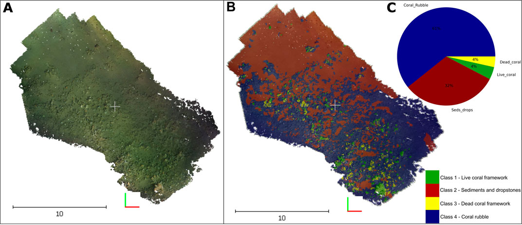
FIGURE 2. (A) Original 3D dense cloud reconstruction of the on-mound section of the Piddington Mound (B) its relative ground-truth labels (C) Percentage class distribution of the reconstructed area.

4.2 Multiclass classification results

4.2.1 Model selection

Results of the grid search show that, from the 18 classifiers, only 6 classifiers or 33.3% obtained accuracies below <60% (red dotted line in Figure 3).

FIGURE 3

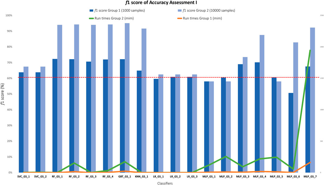
FIGURE 3. Bar plot showing the f1 accuracy results of all 18 classifiers grouped by algorithm type. Light blue bars represent classifiers trained in group 2 (dataset 2, 10,000 samples) and dark blue bars represent classifiers trained in group 1 (dataset 1, 1,000 samples). The red dotted line indicates f1 < 60% threshold. Run times (in minutes) for group 1 (orange) and group 2 (green) represented in the secondary axis on the right are plotted against f1 accuracy.

In order to make an objective comparison of the most efficient classifiers, the classifiers that yielded f1 > 60% on the first accuracy assessment and f1 > 73% (lowest accuracy value obtained) on the second accuracy assessment were selected for an in-depth analysis. Supplementary Table S1 in Supplementary Material summarises the results of the top performing classifiers trained in each group with their respective f1 accuracies of the first accuracy assessment, f1 accuracy of the cross-validation, best combination of parameters from the grid search and finally, the processing time to train each model. The sections below describe the results of the model selection of each of the groups of algorithms trained, including parameter selection, f1 accuracy of group 1 and group 2, accuracy variations and training times.

4.2.1.1 Support Vector Machines

Two SVM classifiers were trained with two different options of kernel parameters. The first SVM (SVC_GS_1), also referred as support vector classifier (SVC) herein, was trained with two choices of kernels: RBF, and sigmoid. The second (SVC_GS_2) with was trained with 3 kernel options: RBF, polynomial and sigmoid. The choice range of the penalty parameter C and the gamma parameter were equal for both. Each of these SVC models was trained in the dataset 1 and dataset 2, resulting on four different trained classifiers: namely SVC_GS_1_1000, SVC_GS_1_10000, SVC_GS_2_1000 and SVC_GS_2_10000. All variations of SVCs chose the combination of 'C': 100, 'gamma': 1, 'kernel': 'rbf' as their best parameters. Among them, the best accuracy SVCs were SVC_GS_1_1000 and SVC_GS_2_10000 (Supplementary Table S1). The accuracy variation between these classifiers across group 1 and group 2 was 3.62% which represented a percentage difference of 5.51% and a 5.67% increase in f1 scores from group 1 to group 2. In addition, the percentage difference on the cross-validation accuracies was of 0.14%.

4.2.1.2 Random Forest

In the four RF classifiers trained, the number of estimators varied at different ranges, going from 10 to 1,000 in steps of 10 or 10 to 100 in steps of 10. Classifiers with the highest accuracies on the first accuracy assessment also held the larger number of estimators (1,000). Among these classifiers the best accuracy RFs on group 1 was RF_GS_1_1000 ('max_features': 1, 'n_estimators': 90) and RF_GS_2_10000 ('max_features': 2, 'n_estimators': 1,000) on group 2 (Supplementary Table S1). The accuracy variation between these classifiers was 21.98% on the first accuracy assessment, which represents a 26.38% difference and a 30.40% increase in accuracy from the best accuracy RF on group 1 to the best accuracy classifiers in the group 2 (Figure 3). The overall intra-model accuracy (RF with same model parameters trained in group 1 and group 2) also showed an increase of 31.16% from RFs trained in group 1 to RF trained in group 2. The difference was less pronounced on the cross-validation accuracies, showing an accuracy difference of 0.67% and only an increase of 0.67% from the RF in group 1 to the RF in group 2. The overall intra-model accuracy difference on the cross-validation assessment was 0.032%. The processing time of the RF_GS_2_10000 was the third longest of all classifiers (2 h 31 min 52 s), staying behind of the top-performing GBT (2 h 52 min 56 s), and MLP (1 day 8 h 25 min 8 s).

4.2.1.3 Gradient Boosting Trees

GBT was the classifier with the highest accuracy among all classifiers, reaching an accuracy of 95.11% on the first accuracy assessment and 80.46% on the cross-validation The top GBT, namely GBT_GS_1_10000 was trained in group 2 with the combination of the parameters: ‘max_depth’: 9, ‘n_estimators’:1,000, ‘subsample’: 0.5, ‘learning_rate’: 0.1. The second GBT, GBT_GS_1_1000 was trained in group 1 and reached an f1 accuracy of 72.15%. The combination of parameters that yielded this classifier was ‘max_depth’: 7, ‘n_estimators’: 1,000, ‘subsample’: 0.7, ‘learning_rate’: 0.1. Both classifiers chose the maximum number of estimators set on the grid search (1,000) (Supplementary Table S1). The accuracy variation between both GBTs on the first accuracy assessment was 22.95%, which represents a 27.45% difference and a 31.81% accuracy increase from the GBT trained in group 1 and the GBT trained in group 2. The cross-validation percentage differences show a much lower gap, with a decrease of <1% (0.16%) from GBT_GS_1_1000 to GS_GS_1_10000. The processing time of the GBT_GS_1_10000 was the second longest of all classifiers (2 h 52 min 56 s), only staying behind of the top-performing MLP (1 day, 8 h 25 min 8 s).

4.2.1.4 k-Nearest Neighbours

The kNN was also among the top-performing classifiers, with a f1 accuracy of 91.6% on the first accuracy assessment and 76.18% on the cross-validation. The first of the two kNNs trained with equal parameters, namely, KNN_GS_1_1000, trained in group 1 resulted in an f1 accuracy of 64.9% and f1 accuracy of 76.02% on the cross-validation. The second kNN was trained in group 2, namely KNN_GS_1_10000, which yielded the aforementioned f1 of 91.6%. Both models chose the same set of parameters: 'metric': 'manhattan', 'n_neighbours': 3, 'weights': 'distance' (Supplementary Table S1). The percentage difference between the accuracies of these classifiers was 34.18%. Overall, the accuracy of the top-performing classifier KNN_GS_1_10000 (group 2) represented an increase of 41.14% on the accuracy relative to the KNN_GS_1_1000 (group 1). kNNs were among the algorithms with the fastest run times, requiring only 2.54s for training of the KNN_GS_1_10000.

4.2.1.5 Logistic Regression

Among the LRs, the best-performing classifiers provided an accuracy of 62.4% and a 74.1% accuracy on the cross-validation for the LR on group 2, namely LR_GS_2_10000. The combination of grid search parameters that resulted in the classifiers were 'C': 100,'Penalty': 'l2','solver': 'sag'. The best LR on group 1 provided an f1 score of 60.95% and 74.01% on the cross-validation. This classifier was created by the grid search with the following set of parameters: 'C': 100,'Penalty': 'l1','solver': 'liblinear' (Supplementary Table S1). The percentage difference between the accuracies of these two classifiers was 2.35%. There was a 2.37% increase in the f`1 accuracy of LR_GS_2_10000 in relation to LR_GS_3_1000. The overall intra-model accuracy (LRs with the same model parameters, but trained in group 1 and group 2) also showed an accuracy increase of 3.21% for LRs trained in group 2, i.e., larger datasets, in comparison to group 1. The overall result put the LRs among the classifiers that yielded the lowest accuracies with an average f1 of 60.51% and 62.4% for LRs in group 1 and group 2, respectively. However, it was also one of the algorithms with the fastest training times (<5 s).

4.2.1.6 Multilayer Perceptrons

Each of the seven generated MLPs was trained in both group 1 and group 2, resulting in a total of 14 trained MLPs. One of these MLPs, the MLP_GS_7_10000 trained in group 2, was among the top four classifiers in this study. The MLP_GS_7_10000 produced an f1 of 92.3% on the first accuracy run and 77.7% on the cross-validation. The combination of parameters that resulted in this classifier were: ‘hidden_layer_sizes’: (200, 200, 200, 200, 200, 200, 200, 200, 200), ‘activation’: ‘tanh’, ‘solver’: ‘adam’, ‘learning rate’: ‘0.0001, ‘max_iter’: 2000, ‘early_stopping’: ‘false’. Among group 1, the best MLP was MLP_GS_4_1000, with an f1 of 70.1% on the first accuracy assessment and 76.9% on the cross-validation. The choice of parameters from the grid search were: hidden_layer_sizes’: (80, 80, 80, 80, 80, 80, 80), ‘activation’: ‘tanh’, ‘solver’: ‘adam’, ‘learning rate’: ‘0.0001, ‘max_iter‘: 2000, ‘early_stopping’: ‘false’ (Supplementary Table S1). The percentage difference of the MLP_GS_7_10000 and the MLP_GS_4_1000 was 27.33%. The first represented a 31.66% f1 increase relative to the latter. The overall intra-model f1 accuracy showed a 16.98% increase in the accuracy of MLPs trained in group 2 (10,000 samples dataset), in relation to group 1 (1,000 samples dataset). The processing time of the MLP_GS_7_10000 was the longest of all classifiers (1 day, 8 h 25 min 8 s), followed by GBT (2 h 52 min 56 s) and RF (2 h 31 min 52 s). It was noted that there was a substantial increase in the run time with the increase of dataset sizes. The classifier MLP_GS_7 had a training time of 2 h 42 min 47 s on group 1. When trained in group 2, the same classifier required took 1 day, 8 h 25 min 8 s to complete its training phase. Considering that the same exact parameters were used, this represents a 1,094.90% increase in the run time. The run time percentage difference of run times between the classifier of best accuracy (GBT_GS_1_10000) and the MLP_GS_7_10000 is 167.34%, which examples the trade-off between run time and accuracy.

4.2.2 Classification output

The classification outputs of the top four classifiers: 1) GBT_GS_1_10000, 2) RF_GS_2_10000 3) MLP_GS_7_10000 and 4) KNN_GS_1_10000 are shown in Figure 4. In this study, classifiers that were above our established threshold of f1 >90% were ranked as the top-performing classifiers. The difference between the classification results and the ground-truth was calculated for each of the aforementioned classifiers (Figure 5).

FIGURE 4

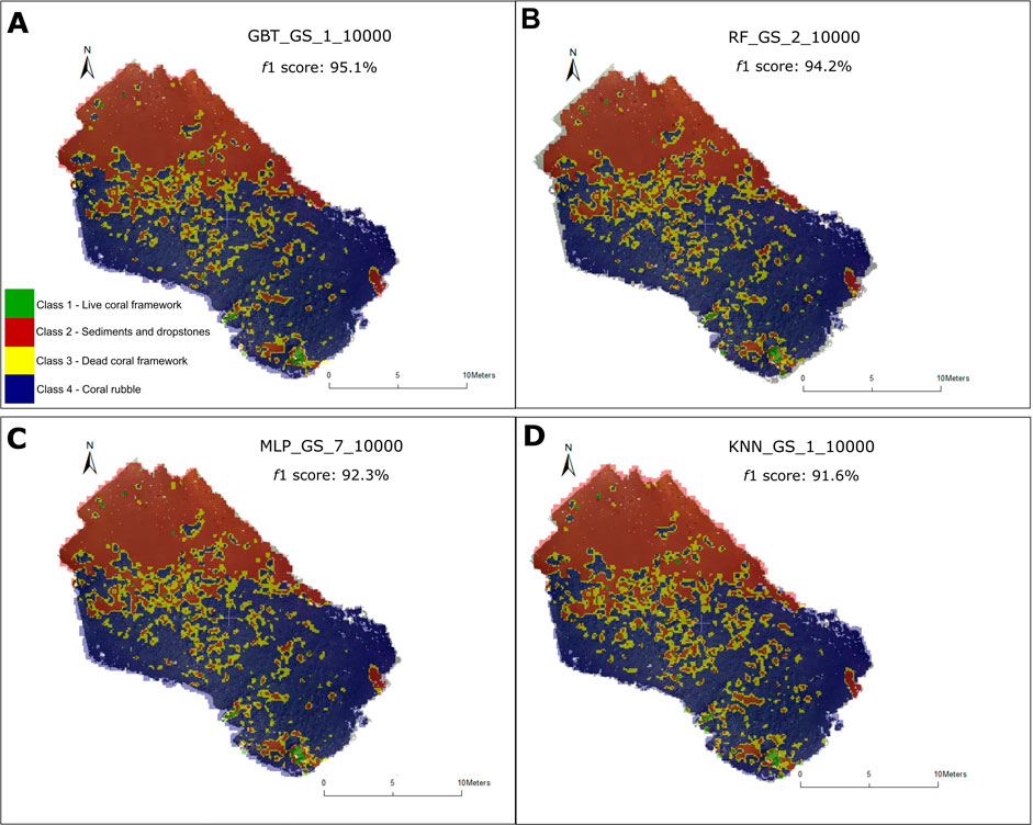
FIGURE 4. Classification outputs of the top four performing classifiers (f1 score > 90%). (A) Classification output of the GBT classifier GBT_GS_1_10000, f1 score: 95.1% (B) Classification output of the RF classifier RF_GS_2_10000, f1 score: 94.2% (C) Classification output of the MLP classifier MLP_GS_7_10000, f1 score: 92.3% (D) Classification output of the KNN classifier KNN_GS_1_10000, f1 score: 91.6%.

FIGURE 5

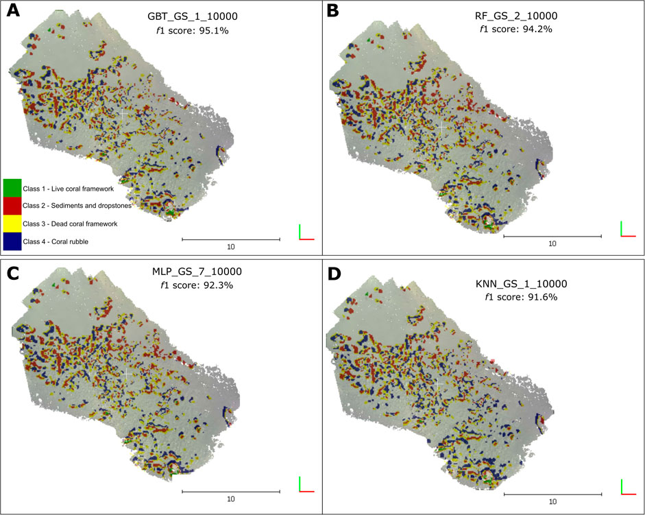
FIGURE 5. Difference of class distribution from the ground-truth labels against the classification output labels of the top four performing classifiers (f1 score > 90%). (A) Difference of classification output vs. ground truth of the GBT classifier GBT_GS_1_10000, f1 score: 95.1% (B) Difference of classification output vs. ground truth of the RF classifier RF_GS_2_10000, f1 score: 94.2% (C) Difference of classification output vs. ground truth of the MLP classifier MLP_GS_7_10000, f1 score: 92.3% (D) Difference of classification output vs. ground truth of the KNN classifier KNN_GS_1_10000, f1 score: 91.6%.

ROC curves were calculated for these classifiers (Figure 6) and AUC scores were calculated for each of the four labels. Points located on the upper right near the X axis typically represent classifiers that make positive classifications based on strong evidence.

FIGURE 6

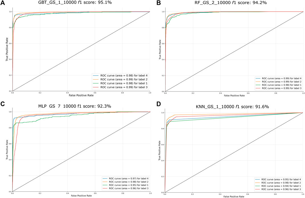
FIGURE 6. ROC curves of the four best-performing classifiers (f1 > 90%). The name of the classifiers and their f1 score obtained on the first accuracy assessment were placed on the top of their respective graph. The AUC score for each label is placed on the lower right side of each graph. Label 1 = LCV, label 2 = SD, label 3 = DCF, label 4 = CR. (A) ROC curve of GBT classifier GBT_GS_1_10000, f1 score: 95.1% (B) ROC curve of the RF classifier RF_GS_2_10000, f1 score: 94.2% (C) ROC curve of the output of the MLP classifier MLP_GS_7_10000, f1 score: 92.3% (D) ROC curve of the KNN classifier KNN_GS_1_10000, f1 score: 91.6%.

Herein, classifiers with the lowest accuracies were those below our established threshold of f1 < 60%. Note that the ROC curves for each label are farther away from the upper left (0, 1) (Figure 7).

FIGURE 7

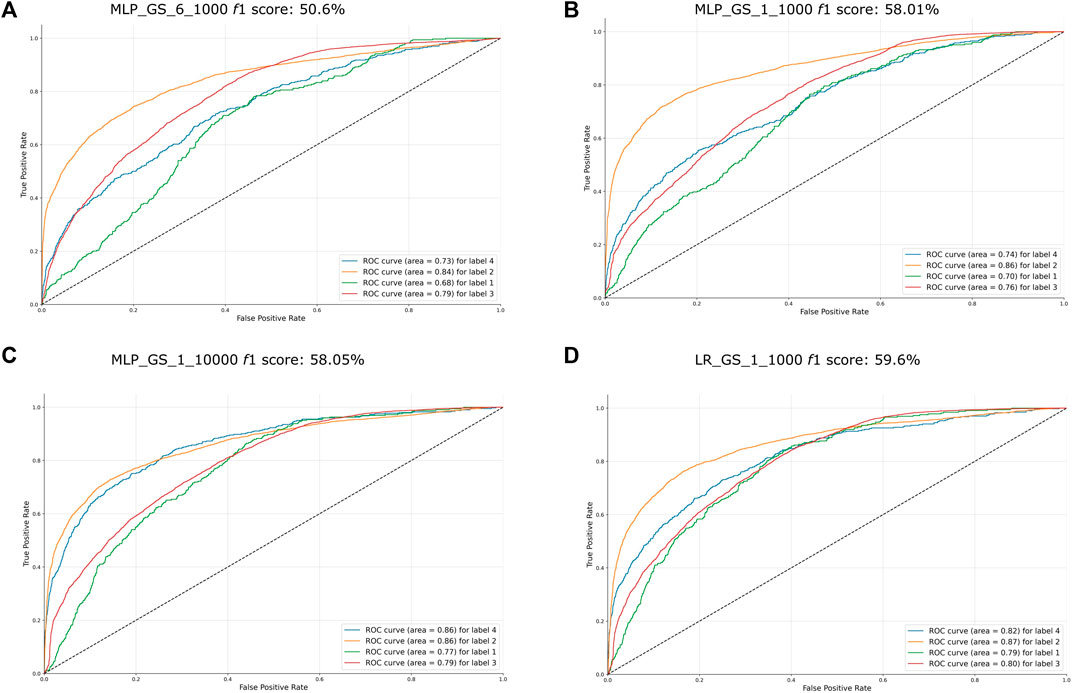
FIGURE 7. ROC curve of the worst performing classifiers (f1 < 60%). The name of the classifiers and their f1 score obtained on the first accuracy assessment were placed on the top their respective graph. The AUC score for each label is placed on the lower right side of each graph. Label 1 = LCF, label 2 = SD, label 3 = DCF, label 4 = CR. (A) ROC curve of MLP classifier MLP_GS_6_1000, f1 score: 50.6% (B) ROC curve of the MLP classifier MLP_GS_1_1000, f1 score: 58.1% (C) ROC curve of output of the MLP classifier MLP_GS_1_10000, f1 score: 58.08% (D) ROC curve of the LR classifier LR_GS_1_1000, f1 score: 59.6%.

5 Discussion

The Piddington Mound is a highly dynamic area with confirmed temporal (Boolukos et al., 2019) and facies changes (Lim et al., 2018a; Conti, Lim, and Wheeler 2019). Studies show that mound surface changed by almost 20% from 2011 to 2015. The CR, DCF, and SD classes showed variations of <7.5%, whereas the LCF remained similar of the 4 years given their inherent slow growth rates (Lim et al., 2018a). Further studies developed at species level found a concerning decline in biodiversity in the same time interval, especially in the percentage coverage of Madrepora oculata with linear decline rates estimated at 0.17%/year (Boolukos et al., 2019). This study shows that, in 2021, this section of the Piddington Mound used had the same proportion of LCF and DCF the on-mound area (4%) followed by the SD class, representing 32% and finally, the class CR which represented the majority of samples (61%) (graph c) Figure 2).

In this study, 241.7 GB worth of data were transformed into an ecologically meaningful and compact dataset (<5.2 gigabytes) that allows for analyses of intra-habitat patterns of the study area. This represents one of the key advantages of 3D photogrammetry and SfM for seabed habitat mapping. Furthermore, 3D reconstructions, orthomosaics and DEMs of CWC derived from video data allows for contextualised analysis of coral colonies and associated fauna (Price et al., 2021). The increasing use of such datasets indicates an advancement in relation to per-image analyses, which may hinder the investigation of spatial patterns, volume density and structural complexity variations.

5.1 Machine learning and 3D reconstructions of coral reef environments

The results show that four ML algorithms yielded f1 accuracies of >90% and were able to successfully discern between classes (Figure 6), especially those with usually similar characteristics, e.g., coral rubble and dead coral, which is a task that is often challenging to both the machine and the human eye (Bryson et al., 2013; Beijbom et al., 2015; Hopkinson et al., 2020). Four algorithms, i.e., LR and three variations of the MLP yielded accuracies below our minimum threshold of 60%. Given the absence of similar studies in 3D photogrammetry and ML in CWC habitats, the results herein contribute to delineating the suitability of specific algorithms for initial assessments, providing key information to future studies in CWC habitats.

5.2 Classifier performance

The classifiers GBT, RF, MLP and kNN trained in group 2 (dataset of 10,000 samples) were the most accurate classifiers on the first assessment, in that order. Nonetheless, the percentage difference between the top-ranked classifier, GBT (f1 = 95.11%) and the fourth-ranked classifier, kNN (f1 = 91.7%) in the first accuracy assessment was low, approximately 3.65%. These results agree with other experimental comparison studies applied to high-resolution satellite imagery for land use/land cover (Jodzani, Johnson, and Chen 2019). Jodzani et al. (2019) showed that MLPs models were the most accurate for those cases. However, there was a small difference in the classification accuracies between these and other algorithms like SVMs and GBTs. Therefore, the use of these algorithms is still versatile to deal with mapping of complex landscapes (Jodzani, Johnson, and Chen 2019). The study also showed that the use of CNNs for the same classification task does not necessarily lead to more accurate results when compared to common classifiers. This agrees with other studies which compared the use of SVMs and sparse auto-encoders for multispectral imagery classifications, where SVMs outperformed auto-encoders (Liu et al., 2017).

Herein, the performance of MLP classifiers trained in this study also agrees with the aforementioned studies. Whilst one of the trained MLPs yielded one of the highest accuracies (MLP_GS_7_10000, f1 score 92.3%), three of the 14 trained MLPs yielded the lowest accuracies (MLP_GS_1_1000, MLP_GS_1_1000, MLP_GS_6_1000) (Figure 3), dropping the overall MLP average performance to 67.62%. Grid search results showed that MLPs were prone to choose hidden layer options with more neurons on them. In addition, all MLP classifiers selected the solver Adam for weight optimization as the final parameter on the grid search. Adam represents a stochastic gradient-based optimizer (Kingma and Lei 2015). The solver is recommended for noisy or sparse gradients and is recommended for problems with large data or parameters (Kingma and Lei 2015). Empirical studies performed in Scikit-learn also suggest that Adam is highly robust for large datasets while converging fast and giving good performances (Buitinck et al., 2013).

RFs have been widely applied for a number of classification tasks in remote sensing (Pal 2005; Rodriguez-Galiano et al., 2012; Belgiu and Drăgu 2016) and specifically, in marine and coastal studies (Seiler et al., 2012; Gauci et al., 2016; Robert et al., 2016; Misiuk et al., 2019; Zelada Leon et al., 2020; Price et al., 2022). In our study, the RF was among the top four classifiers. The f1 score average across all RFs trained was 82.9%. Our analysis showed that using a smaller dataset resulted in models with a lower number of estimators and lower accuracy. However, the suitability of the RF for our classification task can be influenced by a number of factors, one of them is the way RF deals with decision trees in the classification. Studies affirm that RF models reduce the correlation between the decision trees in the ensemble by randomly sampling features, which can lead to an increase in accuracy when compared to other ensemble methods (Jodzani, Johnson, and Chen 2019).

SVMs have been successfully applied for remote sensing applications (Melgani and Bruzzone 2004; Deilmai, Ahmad, and Zabihi 2014; Liu et al., 2017) and automated image analysis (Friedman 2013; Beijbom et al., 2012). In a few cases, SVM-based classifications have outperformed other common classification algorithms, such as kNN and decision trees (Friedman 2013; Beijbom et al., 2012), especially when considering the amount of training data available (Liu et al., 2017). Similar to Friedman (2013) the results herein show that the best-performance SVM was created with RBF kernel. Studies have also suggested that SVM can perform well in cases where there are few training samples (Melgani and Bruzzone 2004). In this study, it was noticed that the SVM were indeed robust with respect to sample size variations, resulting in a small percentage increase of 5.67% when trained in group 1 and group 2. Nonetheless, kernel methods can be sensitive to over-fitting and the kernel choice has been considered the biggest limitation of the SVM approach (Burges 1998; Liu et al., 2017). Although this limitation was addressed by testing a range of kernel options on the grid-search, the SVMs yielded an undistinguished performance on the first accuracy assessment compared to other classifiers. However, they matched the performance of the top four algorithms on the second accuracy assessment, i.e., k-fold cross-validation. It was noted that one of the advantages of the SVM is that, depending on the choice of kernel, the run times are considerably lower when compared to the top four classifiers. However, the kernel choice will have a considerable impact on the processing as there are data limitations when using specific kernels in accordance with the Big O notation (Chivers and Sleightholme 2015). For example, the polynomial kernel is not advised when the dataset has more than 10,000 samples as the SVM training time scales at least quadratically with the number of samples (Tsang, Kwok, and Cheung 2005).

kNNs yielded the 4^th place in our classifiers rank (f1 score = 91.6%) whilst having the lowest training time (2.54 s). Studies performed with ROV-derived images have found that kNN have also outperformed SVMs and NNs in smaller datasets (Shihavuddin et al., 2013). However, when datasets get larger, their effectiveness reduces (Shihavuddin et al., 2013). As mentioned previously, the choice of weighted distance for the kNN can often be evaluated by the similarity across feature dimensions (Russell and Peter 2010). In our grid search results, both kNNs trained in group 1 and group 2 chose Manhattan distance among the parameter grid of the best accuracy models. This suggests that the classifier may have interpreted the feature dimensions as dissimilar. kNNs can suffer with the curse of dimensionality when facing high-dimensionality data (Russell and Peter 2010) therefore, reducing the dimensions of the feature space with, e.g., PCA can increase kNN accuracy (Shihavuddin et al., 2013). A similar issue can happen with the MLPs as, although MLPs can reduce the weight of irrelevant variables close to zero, they may take a long time to converge and consequently, to find a local minimum (Settles and Burr, 2003).

GBT was the most successful classifier in our study, with an f1 accuracy of 95.11% on the first accuracy assessment. Accordingly, studies suggest that GBTs have outstanding performance when compared to RF, SVMs and NN in different classification tasks (Caruana and Niculescu-Mizil 2006; Becker et al., 2018). In studies using bathymetric data to predict diversity and abundance of fish, GBTs were considered the most appropriate technique to select meaningful predictors (Pittman, Costa, and Battista 2009). However, GTBs may be more impacted by the amount of training data in relation to other classifiers, like SVMs. Our study revealed that GBTs had a 31.81% accuracy increase from the GBT trained in group 1 and the GBT trained in group 2, which suggests that the amount of sample data may have a strong impact on the classification. It is also noteworthy this GBT had the second-longest processing time (2 h 52 min 56 s).

Our results show that the LR was among the classifiers with the worst performance on the first accuracy assessment. Studies have shown that the parametric nature of LR classifiers can lead to a more constrained model with limited complexity (Russell and Peter 2010). Previous comparison studies also suggested that Naïve Bayes, logistic regression and variations decision trees are among the poorest-performing algorithms (Caruana and Niculescu-Mizil 2006). However, this is dependent on the type of task performed. Hence, generalisations should be made with caution.

5.3 Sample size and accuracy variation

The quantity of training data is one of the biggest challenges in effectively applying ML for automated seabed mapping (Beijbom et al., 2012; Zurowietz et al., 2018; Williams et al., 2019; Durden et al., 2021). Results on the 1,000 sample dataset and 10,000 sample dataset show that voting ensemble classifiers like kNNs, RF, GBT have better performance and benefit more from a larger dataset than kernel methods such as SVM (Figure 3). The small difference in f1 scores between variations of the same algorithms like SVM (5.51%) and LR (2.35%) suggests that these algorithms are more robust to dataset size variations. As previously mentioned, studies affirm that SVM can perform well in cases where there are few training samples (Melgani and Bruzzone 2004).

Results show that RF is highly sensitive to data size, showing a percentage increase of approximately 30.40% on the average f1 accuracy from 1,000 samples to 10,000 samples datasets. GBT had a 31.81% increase in the average f1 accuracy when trained in 10,000 sample dataset. kNN had a 41.23% increase in the average accuracy when trained in the 10,000 samples dataset. MLPs showed a percentage increase of 16.98% on the accuracy when trained in the 10,000 samples dataset. In contrast, LR showed only a 2.37% increase on the average f1 accuracy. Although this low variation can indicate a positive stability across different sample sizes, it is noteworthy that the LR behaved poorly in all test runs. Similarly, SVMs showed a regular resistance to the dataset variations, with a difference of less than 6% (5.51%) on the average f1 accuracy from group 1 to group 2, noting that the overall performance was also low. The stability of SVMs against different dataset sizes may be due to their ability to handle high-dimensionality data with a relatively low number of training samples (Melgani and Bruzzone 2004; Jodzani, Johnson, and Chen 2019). This is explained by the general concept behind SVMs, which relies on the separation of classes with a maximum plane of separability, using boundary points to create the decision margin, thus making it independent of the dimensionality of feature space (Dixon and Candade 2008).

The number of parameters implies the need for more training samples and computational requirements (Liu et al., 2017). The amount of training data required by NNs increases exponentially with the increase of feature dimensionality of the input data (Dixon and Candade 2008). Similar to automated classification studies with seabed images (Durden et al., 2021), our results show that overall classification is improved by increasing the size of the training dataset.

On the other hand, cross-validation results showed that there is an increase in the f1 scores of the classifiers in group 1. The classifiers trained with 1,000 samples showed a better performance in the f1 accuracy for each fold k in the k-fold cross-validation. The opposite trend was found for group 2, the accuracy dropped and stabilized on the same level as the classifiers of group 1. Therefore, whilst evaluating the performance of the classifiers n parts of the dataset, i.e., cross-validation, the performance of the classifiers of group 1 was similar to the classifiers in group 2. This indicates that in particular instances and metrics, such as when using cross-validation instead of only a single validation set, the classifiers may be used interchangeably. Additionally, cross-validation may be a suitable approach to avoid overfitting when having small sample sets. Overall, In the case of deep-water environments, collecting a large number of labelled samples, dealing with naturally imbalanced datasets and the lack of benchmark data are limitations that need to be overcome in order to advance to the deep learning spectrum (Beijbom et al., 2012; Durden et al., 2021).

The choice of classifiers based on their parametric or non-parametric properties is also important when considering the dataset sizes. In the case of parametric models, such as LR, the number of parameters it needs to make a decision is independent of how much data is used. This property can be useful when datasets are small, as in this case, it is convenient to have a strong constraint on the hypothesis to avoid overfitting (Russell and Peter 2010). However, when the dataset is large, it is better to have more flexible models where the data can have more influence on the learning pattern. Hence, non-parametric models, such as kNNs which cannot be characterized by a delimited set of parameters, can be a better fit. As mentioned, the disadvantage of some non-parametric methods is the amount of data samples necessary.

Another important aspect is the training run times of algorithms in each group. The run times of group 1 algorithms were significantly lower than those in the group 2. It is acknowledged that, despite the fact that MLPs are efficient, the training is time-consuming (Dixon and Candade 2008). A relevant example of run time differences is the classifier MLP_7. Although this MLP had 26.8% decrease in f1 scores when trained in group 1, the run time was 91.63% faster. These results can be taken into consideration when evaluating not only the loss versus run time ratio, but also the processing resources required to run MLPs and the accuracy desired. This is supported by the grid search results, which show that the MLPs yielded similar accuracies in both groups, i.e., independent of the dataset size they were trained with. As NNs, the need for a number of training samples in MLPs can exponentially increase with the dimension of the input of feature space (Dixon and Candade 2008). The results herein contribute to informing the user about the ad hoc strategy to be used when considering the accuracy variation in relation to the processing time. Thus, the user needs to evaluate a set of variables, ranging from the project timeframe, type of object of interest and the computer resources available.

6 Conclusion

Six state-of-art ML classifiers were applied and evaluated for the multiclass classification of high-resolution 3D reconstructions of CWCs environments. A workflow for classification using photogrammetry and ML was proposed for CWC environments of the Irish margin. The multiclass classification results show that certain algorithms proved to be more suited for the specific classification task proposed here, namely: GBTs, RF, kNN, and MLP with f1 > 90. In contrast, the worst-performing classifiers were LR, and two variations of MLP with f1 < 60%. Furthermore, the results suggest that the overall classification is improved by increasing the size of the training dataset. However, it is possible to reach high accuracy results with datasets of 10,000 samples and medium accuracy results with datasets of 1,000 samples. The analysis of the 3D reconstructions shows that, in 2021, this section of the Piddington Mound used had the same proportion of LCF and DCF the on-mound area (4%). The CR class dominated the majority of the samples with 61%, followed by the SD class, representing 32%. The study developed herein shows that ML and photogrammetry enable automated classification of habitats associated with CWC. The proposed workflow will allow for improvements to environmental monitoring strategies by increasing coverage area and optimising data processing.

Data availability statement

The raw data supporting the conclusion of this article will be made available by the authors, without undue reservation.

Author contributions

Conceptualization, LdO and AL; methodology, LdO and AL; software, LdO; validation, LdO and AL; formal analysis, LdO; investigation, LdO; resources, LdO, AL, LC, and AW; data curation, LdO; writing original draft preparation, LdO; writing review and editing, AL, LC, and AW; visualization, LdO; supervision, AL, LC, and AW; project administration, LdO and AW; funding acquisition, LdO, AL, LC, and AW. All authors have read and agreed to the published version of the manuscript.

Funding

This research was funded by Science Foundation Ireland, Geological Survey of Ireland and Marine Institute MMMonKey_Pro project: Grant Number: 16/IA/4528 and the Irish Research Council and Government of Ireland Postgraduate Scholarship Award, ASMaT grant number: GOIPG/2020/1659. LC was supported by São Paulo Research Foundation (Fundação de Amparo à Pesquisa do Estado de São Paulo—FAPESP), grant number: 2017/19649-8. The data collection was funded by Marine Institute 2018 and 2019 Ship Time Program of National Development Scheme in Ireland.

Acknowledgments

The authors would like to thank the Science Foundation Ireland, Geological Survey Ireland and Irish Research Council for funding this work and the first author’s PhD research project. Special thanks go to Marine Institute for funding the ship time on RV Celtic Explorer under the Ship Time Program of the National Development scheme and the shipboard party of RV Celtic Explorer and ROV Holland 1 for their support with data acquisition.

Conflict of interest

The authors declare that the research was conducted in the absence of any commercial or financial relationships that could be construed as a potential conflict of interest.

Publisher’s note

All claims expressed in this article are solely those of the authors and do not necessarily represent those of their affiliated organizations, or those of the publisher, the editors and the reviewers. Any product that may be evaluated in this article, or claim that may be made by its manufacturer, is not guaranteed or endorsed by the publisher.

Supplementary material

The Supplementary Material for this article can be found online at: https://www.frontiersin.org/articles/10.3389/fenvs.2022.1044706/full#supplementary-material

References

Addamo, A. Ma, Vertino, A., Stolarski, J., García-Jiménez, R., Taviani, M., and Machordom, Annie (2016). Merging scleractinian genera: The overwhelming genetic similarity between solitary Desmophyllum and colonial Lophelia. BMC Evol. Biol. 16 (1), 108–117. doi:10.1186/s12862-016-0654-8

PubMed Abstract | CrossRef Full Text | Google Scholar

Agisoft LLC (2020). Agisoft metashape user manual. Professional Edition, St. Petersburg Publisher: Agisoft LLC, 160. https://www.agisoft.com/pdf/metashape-pro_1_7_en.pdf (accessed March 12, 2022).

Google Scholar

Althaus, F., Williams, A., Schlacher, T. A., Kloser, R. J., Green, M. A., Barker, B. A., et al. (2009). Impacts of bottom trawling on deep-coral ecosystems of seamounts are long-lasting. Mar. Ecol. Prog. Ser. 397, 279–294. doi:10.3354/meps08248

CrossRef Full Text | Google Scholar

Appah, J. K. M., Lim, A., Harris, K., O’Riordan, R., O’Reilly, L., Wheeler, A. J., et al. (2020). Are non-reef habitats as important to benthic diversity and composition as coral reef and rubble habitats in Submarine Canyons? Analysis of controls on benthic megafauna distribution in the Porcupine Bank Canyon, NE Atlantic. Front. Mar. Sci. 7, 831. doi:10.3389/fmars.2020.571820

CrossRef Full Text | Google Scholar

Becker, C, E., Häni, N., d’Angelo, E., and Strecha, C. (2018). Classification of aerial photogrammetric 3D point clouds. Photogramm. Eng. remote Sens. 84 (5), 287–295. doi:10.14358/PERS.84.5.287

CrossRef Full Text | Google Scholar

Beijbom, O., Edmunds, P. J., Roelfsema, C., Smith, J., Kline, D. I., Neal, B. P., et al. (2015). Towards automated annotation of benthic survey images: Variability of human experts and operational modes of automation. PLoS ONE 10 (7), e0130312–e0130322. doi:10.1371/journal.pone.0130312

PubMed Abstract | CrossRef Full Text | Google Scholar

Beijbom, O., Peter, J., Kline, D. I., Mitchell, B. G., and Kriegman, D. (2012). Automated annotation of coral reef survey images. Proc. IEEE Comput. Soc. Conf. Comput. Vis. Pattern Recognit., 1170. –77. doi:10.1109/CVPR.2012.6247798

CrossRef Full Text | Google Scholar

Belgiu, M., and Drăgu, L. (2016). Random forest in remote sensing: A review of applications and future directions. ISPRS J. Photogrammetry Remote Sens. 114, 24–31. doi:10.1016/j.isprsjprs.2016.01.011

CrossRef Full Text | Google Scholar

Bergh, J. v. d., Chirayath, V., Li, A., Torres-Pérez, J. L., and Segal-Rozenhaimer, M. (2021). NeMO-net – gamifying 3D labeling of multi-modal reference datasets to support automated marine habitat mapping. Front. Mar. Sci. 8. doi:10.3389/fmars.2021.645408

CrossRef Full Text | Google Scholar

Bishop, C. M. (2006). Pattern recognition and machine learning. Information science and statistics. New York: Springer. https://link.springer.com/book/9780387310732.

Google Scholar

Boolukos, C. M., Lim, A., O’Riordan, R. M., and Wheeler, A. J. (2019). Cold-water corals in decline – a temporal (4 Year) species abundance and biodiversity appraisal of complete photomosaiced cold-water coral reef on the Irish margin. Deep Sea Res. Part I Oceanogr. Res. Pap. 146, 44–54. doi:10.1016/j.dsr.2019.03.004

CrossRef Full Text | Google Scholar

Bryson, M., Johnson-Roberson, M., Pizarro, O., and Williams, S. B. (2013). Colour-consistent structure-from-motion models using underwater imagery. Robotics Sci. Syst. 8, 33–40. doi:10.7551/mitpress/9816.003.0010

CrossRef Full Text | Google Scholar

Buda, M., Maki, A., and Macieji, A. (2018). A systematic study of the class imbalance problem in convolutional neural networks. Neural Netw. 106, 249–259. doi:10.1016/j.neunet.2018.07.011

PubMed Abstract | CrossRef Full Text | Google Scholar

Buhl-Mortensen, L., Gooday, A. J., Levin, L. A., Priede, I. G., Buhl-Mortensen, P., et al. (2010). Biological structures as a source of habitat heterogeneity and biodiversity on the deep ocean margins. Mar. Ecol. 31 (1), 21–50. doi:10.1111/j.1439-0485.2010.00359.x

CrossRef Full Text | Google Scholar

Buitinck, L., Louppe, G., Blondel, M., Pedregosa, F., Mueller, A., Grisel, O., et al. (2013). API design for machine learning software: Experiences from the scikit-learn project, 1–15. http://arxiv.org/abs/1309.0238.

PubMed Abstract | Google Scholar

Burges, C. J. C. (1998). A tutorial on support vector machines for pattern recognition. Data Min. Knowl. Discov. 28, 121–167. doi:10.1023/a:1009715923555

CrossRef Full Text | Google Scholar

Burns, D., Gates, R. D., and Takabayashi, M. (2015a). Integrating structure-from-motion photogrammetry with geospatial software as a novel technique for quantifying 3D ecological characteristics of coral reefs. PeerJ 2015 (7), e1077. doi:10.7717/peerj.1077

PubMed Abstract | CrossRef Full Text | Google Scholar

Burns, J. H. R., Delparte, D., Gates, R. D., and Takabayashi., M. (2015b). Utilizing underwater three-dimensional modeling to enhance ecological and biological studies of coral reefs. Int. Arch. Photogramm. Remote Sens. Spat. Inf. Sci., 61–66. XL-5/W5 (5W5): 61–66. doi:10.5194/isprsarchives-XL-5-W5-61-2015

CrossRef Full Text | Google Scholar

Calders, K., Stuart, P., Ferrari, R., Leon, J., Armston, J., Asner, G. P., et al. (2020). 3D imaging insights into Forests and coral reefs. Trends Ecol. Evol. 35 (1), 6–9. doi:10.1016/j.tree.2019.10.004

PubMed Abstract | CrossRef Full Text | Google Scholar

Carrivick, J. L., Smith, M. W., and Quincey, D. J. (2016). Structure from motion in the geosciences. Chichester, UK: John Wiley & Sons. doi:10.1002/9781118895818

CrossRef Full Text | Google Scholar

Caruana, R., and Niculescu-Mizil, A. (2006). “An empirical comparison of supervised learning algorithms,” in ICML 2006 - Proceedings of the 23rd International Conference on Machine Learning, 161–168.

CrossRef Full Text | Google Scholar

Castelvecchi, D. (2016). The black box of AI. Nature 538 (7623), 20–23. doi:10.1038/538020a

PubMed Abstract | CrossRef Full Text | Google Scholar

Chawla, N. V., Bowyer, K. W., Hall, L. O., and Philip Kegelmeyer, W. 2002. “Smote: Synthetic minority over-sampling technique.” jair. 16, 321. doi:10.1613/jair.953

CrossRef Full Text | Google Scholar

Chivers, I., and Sleightholme, J. (2015). “An introduction to algorithms and the Big O notation,” in Introduction to programming with fortran: With coverage of fortran 90. Third Edition (Cham: Springer International Publishing), 95, 771–674. doi:10.1007/978-3-319-17701-4

CrossRef Full Text | Google Scholar

Clippele, L. H., Ramiro-Sánchez, B., Kazanidis, G. J. Vad, S. Turner, R. N. Glud, and Roberts, J. M. (2021). Mapping cold-water coral biomass: An approach to derive ecosystem functions. Coral Reefs 40 (1), 215–231. doi:10.1007/s00338-020-02030-5

CrossRef Full Text | Google Scholar

Cocito, S., Sgorbini, S., Peirano, A., and Valle, M. (2003). 3-D reconstruction of biological objects using underwater video technique and image processing. J. Exp. Mar. Biol. Ecol. 297 (1), 57–70. doi:10.1016/S0022-0981(03)00369-1

CrossRef Full Text | Google Scholar

Conti, L. A., Lim, A., and Wheeler, A. J. (2019). High resolution mapping of a cold water coral mound. Sci. Rep. 9 (1), 1016. doi:10.1038/s41598-018-37725-x

PubMed Abstract | CrossRef Full Text | Google Scholar

Costello, M. J., McCrea, M., Freiwald, A., Lundälv, T., Jonsson, L., Bett, B. J., et al. (2005). “Role of cold-water Lophelia pertusa coral reefs as fish habitat in the NE atlantic,” in Cold-water corals and ecosystems (Springer Berlin Heidelberg), 771–805. doi:10.1007/3-540-27673-4_41

CrossRef Full Text | Google Scholar

Courtney, L. A., Fisher, W. S., Raimondo, S., Oliver, L. M., and Davis, W. P. (2007). Estimating 3-dimensional colony surface area of field corals. J. Exp. Mar. Biol. Ecol. 351 (1–2), 234–242. doi:10.1016/j.jembe.2007.06.021

CrossRef Full Text | Google Scholar

Deilmai, B. R., Ahmad, B. B., and Zabihi, H. (2014). Comparison of two classification methods (MLC and SVM) to extract land use and land cover in johor Malaysia. IOP Conf. Ser. Earth Environ. Sci. 20 (1), 012052. doi:10.1088/1755-1315/20/1/012052

CrossRef Full Text | Google Scholar

Dixon, B., and Candade, N. (2008). Multispectral landuse classification using neural networks and support vector machines: One or the other, or both? Int. J. Remote Sens. 29 (4), 1185–1206. doi:10.1080/01431160701294661

CrossRef Full Text | Google Scholar

Dorey, N., Gjelsvik, Ø., Kutti, T., and Janina, V. (2020). Broad thermal tolerance in the cold-water coral Lophelia pertusa from arctic and boreal reefs. Front. Physiol. 10, 1636–1712. doi:10.3389/fphys.2019.01636

PubMed Abstract | CrossRef Full Text | Google Scholar

Dorschel, B., Hebbeln, D., Foubert, A., White, M., and Wheeler, A. J. (2007). Hydrodynamics and cold-water coral facies distribution related to recent sedimentary processes at Galway mound west of Ireland. Mar. Geol. 244 (1–4), 184–195. doi:10.1016/j.margeo.2007.06.010

CrossRef Full Text | Google Scholar

Dorschel, B. (2003). Late quaternary development of a deep-water carbonate mound in the northeast atlantic. PhD Thesis, 90. Geowissenschaften PhD.

Google Scholar

Durden, J. M., Brett Hosking, B., and Ruhl, H. A. (2021). Automated classification of fauna in seabed photographs: The impact of training and validation dataset size, with considerations for the class imbalance. Prog. Oceanogr. 196, 102612. doi:10.1016/j.pocean.2021.102612

CrossRef Full Text | Google Scholar

Fawcett, T. (2006). An introduction to ROC analysis. Pattern Recognit. Lett. 27 (8), 861–874. doi:10.1016/j.patrec.2005.10.010

CrossRef Full Text | Google Scholar

Ferrari, R., Figueira, W. F., Pratchett, M. S., Boube, T., Adam, A., and Byrne, M. (2017). 3D photogrammetry quantifies growth and external erosion of individual coral colonies and skeletons. Sci. Rep. 7 (1), 16737–16739. doi:10.1038/s41598-017-16408-z

PubMed Abstract | CrossRef Full Text | Google Scholar

Figueira, W., Ferrari, R., Weatherby, E., Porter, Ae, Hawes, S., and Byrne, M. (2015). Accuracy and precision of habitat structural complexity metrics derived from underwater photogrammetry. Remote Sens. 7 (12), 16883–16900. doi:10.3390/rs71215859

CrossRef Full Text | Google Scholar

Fosså, J. H., Mortensen, P. B., and Furevik, D. M. (2002). The deep-water coral Lophelia pertusa in Norwegian waters: Distribution and fishery impacts. Hydrobiologia 471, 1–12. doi:10.1023/A:1016504430684

CrossRef Full Text | Google Scholar

Foubert, A., Beck, T., Wheeler, A. J., Jan, O., Grehan, A., Klages, M., et al. (2006). “New view of the Belgica mounds, porcupine Seabight, NE atlantic: Preliminary results from the polarstern ARK-XIX/3a ROV cruise,” in Cold-water corals and ecosystems (Berlin/Heidelberg: Springer-Verlag), 403–15. doi:10.1007/3-540-27673-4_20

PubMed Abstract | CrossRef Full Text | Google Scholar

Foubert, A., Huvenne, V. A. I., Wheeler, A., Kozachenko, M., Opderbecke, J., and Henriet, J.-P. (2011). The Moira mounds, small cold-water coral mounds in the porcupine Seabight, NE atlantic: Part B—evaluating the impact of sediment dynamics through high-resolution ROV-borne bathymetric mapping. Mar. Geol. 282 (1–2), 65–78. doi:10.1016/j.margeo.2011.02.008

CrossRef Full Text | Google Scholar

Freiwald, A., and Roberts, J. M. (2005). Cold-water corals and ecosystems. Springer Berlin Heidelberg. doi:10.1007/3-540-27673-4

CrossRef Full Text | Google Scholar

Freiwald, A. (2002). “Reef-forming cold-water corals,” in Ocean margin systems (Springer Berlin Heidelberg), 365–85. doi:10.1007/978-3-662-05127-6_23

PubMed Abstract | CrossRef Full Text | Google Scholar

Friedman, A. (2013). Automated interpretation of benthic stereo imagery. University of Sydney.

Google Scholar

Friedman, J. H. (2001). Greedy function approximation: A gradient boosting machine. Ann. Stat. 29 (5), 1189–1232. doi:10.1214/aos/1013203451

CrossRef Full Text | Google Scholar

Fu, T., Ma, L., Li, M., and Brian, A. (2018). Using convolutional neural network to identify irregular segmentation objects from very high-resolution remote sensing imagery. J. Appl. Rem. Sens. 12 (02), 1. doi:10.1117/1.jrs.12.025010

CrossRef Full Text | Google Scholar

Fukunaga, A., and Burns, J. H. R. (2020). Metrics of coral reef structural complexity extracted from 3D mesh models and digital elevation models. Remote Sens. 12 (17), 2676. doi:10.3390/RS12172676

CrossRef Full Text | Google Scholar

Gauci, A., Deidun, A., and Abela, J. (2016). Machine learning for benthic sand and maerl classification and coverage estimation in coastal areas around the Maltese islands. J. Appl. Res. Technol. 14 (5), 338–344. doi:10.1016/j.jart.2016.08.003

CrossRef Full Text | Google Scholar

Gilardi, Nicolas (1995). Comparison of four machine learning algorithms for spatial data analysis. Evaluation 1–16.

PubMed Abstract | Google Scholar

Goatley, C. H. R., and Bellwood, D. R. (2011). The roles of dimensionality, canopies and complexity in ecosystem monitoring. PLoS ONE 6 (11), e27307. doi:10.1371/journal.pone.0027307

PubMed Abstract | CrossRef Full Text | Google Scholar

González-Rivero, M., Beijbom, O., Rodriguez-Ramirez, A., Dominic, E., Bryant, P., et al. (2020). Anjani Ganase, Yeray Gonzalez-Marrero, Ana Herrera-Reveles, et alMonitoring of Coral Reefs Using Artificial Intelligence: A Feasible and Cost-Effective Approach. Remote Sens. 12 (3), 489–522. doi:10.3390/rs12030489

CrossRef Full Text | Google Scholar

Gori, A., Ferrier-Pagès, C., Hennige, S. J., Murray, F., Rottier, C., Wicks, L. C., et al. (2016). Physiological response of the cold-water coral Desmophyllum dianthus to thermal stress and ocean acidification. PeerJ 2016 (2), e1606–e1616. doi:10.7717/peerj.1606

PubMed Abstract | CrossRef Full Text | Google Scholar

Graham, N. A. J., and Nash, K. L. (2013). The importance of structural complexity in coral reef ecosystems. Coral Reefs 32 (2), 315–326. doi:10.1007/s00338-012-0984-y

CrossRef Full Text | Google Scholar

Guinan, J., Grehan, A. J., Dolan, M. F. J., and Brown, C. (2009). Quantifying relationships between video observations of cold-water coral cover and seafloor features in rockall trough, west of Ireland. Mar. Ecol. Prog. Ser. 375, 125–138. doi:10.3354/meps07739

CrossRef Full Text | Google Scholar

Gutierrez-Heredia, L., Benzoni, F., Murphy, E., and Reynaud, E. G. (2016). End to end digitisation and analysis of three-dimensional coral models, from communities to corallites. PLoS ONE 11 (2), e0149641. doi:10.1371/journal.pone.0149641

PubMed Abstract | CrossRef Full Text | Google Scholar

Hengl, T., Nussbaum, M., Wright, M. N., Heuvelink, G. B. M., and Gräler, Benedikt (2018). Random forest as a generic framework for predictive modeling of spatial and spatio-temporal variables. PeerJ 2018 (8), e5518. doi:10.7717/peerj.5518

PubMed Abstract | CrossRef Full Text | Google Scholar

Henry, L. A., and Murray Roberts, J. (2017). “Global biodiversity in cold-water coral reef ecosystems,” in Marine animal Forests: The ecology of benthic biodiversity hotspots (Springer International Publishing), 235–56. doi:10.1007/978-3-319-21012-4_6

PubMed Abstract | CrossRef Full Text | Google Scholar

Hopkinson, B. M., KingOwenJohnson-Roberson, A. C. D. P. M., Long, M. H., Bhandarkar, Suchendra M., Long, M. H., and Bhandarkar, S. M. (2020). Automated classification of three-dimensional reconstructions of coral reefs using convolutional neural networks. PLoS ONE 15 (3), e0230671. doi:10.1371/journal.pone.0230671

PubMed Abstract | CrossRef Full Text | Google Scholar

House, J. E., Viviana Brambilla, L. M., Pizarro, O., Madin, J. S., Dornelas, M., Madin, J. S., et al. (2018). Moving to 3D: Relationships between coral planar area, surface area and volume. Surf. Area PeerJ 2018 (2), e4280. doi:10.7717/peerj.4280

PubMed Abstract | CrossRef Full Text | Google Scholar

Huang, Z., Brooke, B. P., and Harris, P. T. (2011). A new approach to mapping marine benthic habitats using physical environmental data. Cont. Shelf Res. 31 (31), 4–16. doi:10.1016/j.csr.2010.03.012

CrossRef Full Text | Google Scholar

Huvenne, V. A. I., Blondel, Ph, and Henriet, J. P. (2002). Textural analyses of sidescan sonar imagery from two mound provinces in the porcupine Seabight. Mar. Geol. 189 (3–4), 323–341. doi:10.1016/S0025-3227(02)00420-6

CrossRef Full Text | Google Scholar

Jodzani, S. E., Brian, J. E., and Chen, D. (2019). Comparing deep neural networks , ensemble classifiers , and support vector machine algorithms. Remote Sens. 11 (1), 1–24. doi:10.3390/rs11141713

CrossRef Full Text | Google Scholar

Karara, G., Hajji, R., and Poux, F. (2021). 3D point cloud semantic augmentation: Instance segmentation of 360° panoramas by deep learning techniques. Remote Sens. 13 (18), 3647. doi:10.3390/rs13183647

CrossRef Full Text | Google Scholar

Kingma, D. P., and Lei, J. (2015). “Adam: A method for stochastic optimization,” in 3rd International Conference on Learning Representations, ICLR 2015 (Conference Track Proceedings).1–15

PubMed Abstract | Google Scholar

Kornder, N. A., Cappelletto, J., Mueller, B., Zalm, M. J. L., Stephanie, J., Martinez, M. J. A. V., et al. (2021). Implications of 2D versus 3D surveys to measure the abundance and composition of benthic coral reef communities. Coral Reefs 40, 1137–1153. doi:10.1007/s00338-021-02118-6

PubMed Abstract | CrossRef Full Text | Google Scholar

Lange, I. D., and Perry, C. T. (2020). A quick, easy and non-invasive method to quantify coral growth rates using photogrammetry and 3D model comparisons. Methods Ecol. Evol. 11 (6), 714–726. doi:10.1111/2041-210X.13388

CrossRef Full Text | Google Scholar

Last, F., Douzas, G., and Bacao, F. (2017). Oversampling for imbalanced learning based on K-means and SMOTE. 1–19. doi:10.1016/j.ins.2018.06.056

CrossRef Full Text | Google Scholar

Leon, J. X., Roelfsema, C. M., Saunders, M. I., and Phinn, S. R. (2015). Measuring coral reef terrain roughness using ‘structure-from-motion’ close-range photogrammetry. Geomorphology 242, 21–28. doi:10.1016/j.geomorph.2015.01.030

CrossRef Full Text | Google Scholar

Lim, A., Adam, K., Arnaubec, A., and Andrew, J. (2018b). Seabed image acquisition and survey design for cold water coral mound characterisation. Mar. Geol. 395, 22–32. doi:10.1016/j.margeo.2017.09.008

CrossRef Full Text | Google Scholar

Lim, A., Huvenne, V. A. I., Vertino, A., Spezzaferri, S., and Wheeler, A. J. (2018a). New insights on coral mound development from groundtruthed high-resolution ROV-mounted multibeam imaging. Mar. Geol. 403, 225–237. doi:10.1016/j.margeo.2018.06.006

CrossRef Full Text | Google Scholar

Lim, A., O’Reilly, L., Macêdo Cruz de Oliveira, L., and Strachan, R. (2020a). CE20011 cruise report: Systematic monitoring survey of the Moira mound chain (SyMonS_MoM). https://www.ucc.ie/en/media/research/marinegeo/mgpdfs/SyMonS_MoM__CE20011_Cruise_Report.pdf.

Google Scholar

Lim, A. (2017). Spatio – temporal patterns and controls on cold-water coral reef development : The Moira mounds. Offshore Ireland: Porcupine Seabight.

Google Scholar

Lim, A., Wheeler, A. J., Price, D. M., O’Reilly, L., Harris, K., and Conti, L. (2020c). Influence of benthic currents on cold-water coral habitats: A combined benthic monitoring and 3D photogrammetric investigation. Sci. Rep. 10 (1), 19433. doi:10.1038/s41598-020-76446-y

PubMed Abstract | CrossRef Full Text | Google Scholar

Lim, A., Wheeler, A. J., and Arnaubec, A. (2017). High-resolution facies zonation within a cold-water coral mound: The case of the Piddington mound, porcupine Seabight, NE atlantic. Mar. Geol. 390, 120–130. doi:10.1016/j.margeo.2017.06.009

CrossRef Full Text | Google Scholar

Lim, A., Wheeler, A. J., and Conti, L. (2020b). Cold-water coral habitat mapping: Trends and developments in acquisition and processing methods. Geosciences 11 (1), 9. doi:10.3390/geosciences11010009

CrossRef Full Text | Google Scholar

Liu, P., Kim, K., Wang, L., and Huang, F. (2017). SVM or deep learning? A comparative study on remote sensing image classification. Soft Comput. 21 (23), 7053–7065. doi:10.1007/s00500-016-2247-2

CrossRef Full Text | Google Scholar

Lowe, D. G. (1999). “Object recognition from local scale-invariant features,” in Proceedings of the Seventh IEEE International Conference on Computer Vision (IEEE), 1150–1572. doi:10.1109/ICCV.1999.790410

CrossRef Full Text | Google Scholar

Luckhurst, B. E., and Luckhurst, K. (1978). Analysis of the influence of substrate variables on coral reef fish communities. Mar. Biol. 49 (4), 317–323. doi:10.1007/BF00455026

CrossRef Full Text | Google Scholar

Ma, L., Li, M., Ma, X., Cheng, L., Du, P., and Liu, Yongxue (2017). A review of supervised object-based land-cover image classification. ISPRS J. Photogrammetry Remote Sens. 130, 277–293. doi:10.1016/j.isprsjprs.2017.06.001

CrossRef Full Text | Google Scholar

Mahmood, A., Bennamoun, M., An, S., Sohel, F. A., Boussaid, F., Hovey, Re, et al. (2019). Deep image representations for coral image classification. IEEE J. Ocean. Eng. 44 (1), 121–131. doi:10.1109/JOE.2017.2786878

CrossRef Full Text | Google Scholar

Melgani, F., and Bruzzone, L. (2004). Classification of hyperspectral remote sensing–90, 1778.

CrossRef Full Text | Google Scholar

Misiuk, B., Diesing, M., Aitken, A., Brown, C. J., Edinger, Evan N., and Bell., Trevor (2019). A spatially explicit comparison of quantitative and categorical modelling approaches for mapping seabed sediments using random forest. Geosci. Switz. 9 (6), 254–334. doi:10.3390/geosciences9060254

CrossRef Full Text | Google Scholar

Modasshir, Md, Rahman, S., Youngquist, O., and Rekleitis, I. (2018). “Coral identification and counting with an autonomous underwater vehicle,” in 2018 IEEE international conference on robotics and biomimetics ROBIO (December, 2018, 524–529. doi:10.1109/ROBIO.2018.8664785

CrossRef Full Text | Google Scholar

Mohamed, H., Nadaoka, K., and Nakamura, T. (2022). Automatic semantic segmentation of benthic habitats using images from towed underwater camera in a complex shallow water environment, 1–22.

PubMed Abstract | Google Scholar

Mohamed, H., Nadaoka, K., and Nakamura, T. (2020). Towards benthic habitat 3D mapping using machine learning algorithms and structures from motion photogrammetry. Remote Sens. 12 (1), 127. doi:10.3390/rs12010127

CrossRef Full Text | Google Scholar

Mol, B. De, Kozachenko, M., Wheeler, A., Alvares, H., Henriet, J., and Olu-Le Roy, K. (2007). Thérèse mound: A case study of coral bank development in the Belgica mound province, porcupine Seabight. Int. J. Earth Sci. 96 (1), 103–120. doi:10.1007/s00531-005-0496-x

CrossRef Full Text | Google Scholar

Mortensen, L., Martin, H., Brattegard, T., and Farestveit, R. (1995). Deep water bioherms of the scleractinian coral Lophelia pertusa (L.) at 64° n on the Norwegian shelf: Structure and associated megafauna. Sarsia 80 (2), 145–158. doi:10.1080/00364827.1995.10413586

CrossRef Full Text | Google Scholar

Mountrakis, Giorgos, Jungho, Im, and Ogole, Caesar (2011). Support vector machines in remote sensing: A review. ISPRS J. Photogrammetry Remote Sens. 66 (3), 247–259. doi:10.1016/j.isprsjprs.2010.11.001

CrossRef Full Text | Google Scholar

Oliveira, L., Lim, A., Conti, L. A., and Wheeler, A. J. (2021). 3D classification of cold-water coral reefs: A comparison of classification techniques for 3D reconstructions of cold-water coral reefs and seabed. Front. Mar. Sci. 8. doi:10.3389/fmars.2021.640713

CrossRef Full Text | Google Scholar

Pal, M. (2005). Random forest classifier for remote sensing classification. Int. J. Remote Sens. 26 (1), 217–222. doi:10.1080/01431160412331269698

CrossRef Full Text | Google Scholar

Pascoe, K. H., Fukunaga, A., Kosaki, R. K., and Burns, J. H. R. (2021). 3D assessment of a coral reef at lalo atoll reveals varying responses of habitat metrics following a catastrophic hurricane. Sci. Rep. 11 (1), 12050. doi:10.1038/s41598-021-91509-4

PubMed Abstract | CrossRef Full Text | Google Scholar

Pedregosa, F., Varoquaux, G., Gramfort, A., Michel, V., Bertrand, T., Grisel, O., et al. (2011). Scikit-Learn: Machine learning in Python. J. Mach. Learn. Res. 12, 2825–2830.

Google Scholar

Pierce, J., Butler, M. J. I. V., Rzhanov, Y., Kim, L., and Jennifer, A. (2021). Classifying 3-D models of coral reefs using structure-from-motion and multi-view semantic segmentation. Front. Mar. Sci. 0, 1623. doi:10.3389/FMARS.2021.706674

CrossRef Full Text | Google Scholar

Pittman, Sn J., Costa, B. M., and Tim, A. (2009). Using lidar bathymetry and boosted regression trees to predict the diversity and abundance of fish and corals. J. Coast. Res. 10053, 27–38. doi:10.2112/si53-004.1

CrossRef Full Text | Google Scholar

Pizarro, O., Friedman, A., Bryson, M., Williams, S. B., and Madin, J. (2017). A simple, fast, and repeatable survey method for underwater visual 3D benthic mapping and monitoring. Ecol. Evol. 7 (6), 1770–1782. doi:10.1002/ece3.2701

PubMed Abstract | CrossRef Full Text | Google Scholar

Poux, F., Neuville, R., and Gilles, A. (2018). 3D point cloud semantic modelling: Integrated framework for indoor spaces and furniture. Remote Sens. 10 (9), 1412. doi:10.3390/rs10091412

CrossRef Full Text | Google Scholar

Price, D. M., Felgate, S. L., Huvenne, V. A. I., James, S., Carpenter, S., Barry, C., et al. (2022). Quantifying the intra-habitat variation of seagrass beds with unoccupied aerial Vehicles ( UAVs ).

Google Scholar

Price, D. M., Lim, A., Callaway, A., Eichhorn, M. P., Wheeler, A. J., Lo Iacono, Cl, et al. (2021). Fine-scale heterogeneity of a cold-water coral reef and its influence on the distribution of associated taxa. Front. Mar. Sci. 8. doi:10.3389/fmars.2021.556313

CrossRef Full Text | Google Scholar

Price, K. R., Callaway, A., Lo lacono, C., Hall, R. A., Huvenne, A. I., and Huvenne, V. A. I. (2019). Using 3D photogrammetry from ROV video to quantify cold-water coral reef structural complexity and investigate its influence on biodiversity and community assemblage. Coral Reefs 38 (5), 1007–1021. doi:10.1007/s00338-019-01827-3

CrossRef Full Text | Google Scholar

Qi, C. R., Su, H., Mo, K., and Leonidas, J. (2017). “PointNet: Deep learning on point sets for 3D classification and segmentation,” in Proceedings - 30th IEEE Conference on Computer Vision and Pattern Recognition. CVPR 2017 2017-Janua: 77–85. doi:10.1109/CVPR.2017.16

CrossRef Full Text | Google Scholar

Robert, K., Jones, B., Roberts, J. M., and Huvenne, V. A. I. (2016). Improving predictive mapping of deep-water habitats: Considering multiple model outputs and ensemble techniques. Deep Sea Res. Part I Oceanogr. Res. Pap. 113, 80–89. doi:10.1016/j.dsr.2016.04.008

CrossRef Full Text | Google Scholar

Roberts, J. M., Wheeler, A., Freiwald, A., and Cairns, S. (2009). Cold-water corals. Cambridge University Press. doi:10.1017/CBO9780511581588

CrossRef Full Text | Google Scholar

Roberts, J. M., Harvey, S. M., Lamont, P. A., Gage, J. D., and Humphery, J. D. (2000). Seabed photography, environmental assessment and evidence for deep-water trawling on the continental margin west of the hebrides. Hydrobiologia 441, 173–183. doi:10.1023/A:1017550612340

CrossRef Full Text | Google Scholar

Rodriguez-Galiano, V. F., Ghimire, B., Rogan, J., Chica-Olmo, M., and Rigol-Sanchez, J. P. (2012). An assessment of the effectiveness of a random forest classifier for land-cover classification. ISPRS J. Photogrammetry Remote Sens. 67 (1), 93–104. doi:10.1016/j.isprsjprs.2011.11.002

CrossRef Full Text | Google Scholar

Roelfsema, C. M., Lyons, M., Murray, N., Kovacs, E. M., Kennedy, E., Markey, K., et al. (2021). Workflow for the generation of expert-derived training and validation data: A view to global scale habitat mapping. Front. Mar. Sci. 8, 643381. doi:10.3389/fmars.2021.643381

CrossRef Full Text | Google Scholar

Rogers, A. (1999). The biology of Lophelia pertusa (linnaeus 1758) and other deep-water reef-forming corals and impacts from human activities. Int. Rev. Hydrobiology 84 (4), 315–406. doi:10.1002/iroh.199900032

CrossRef Full Text | Google Scholar

Rudall, B. H. (1978). Lecture notes in computer science. Vol. 15—L-Systems. Int. J. Bio-Medical Comput. 9 (3), 242. doi:10.1016/0020-7101(78)90038-7

CrossRef Full Text | Google Scholar

Russell, S. J., and Peter, N. (2010). Artificial intelligence: A modern approach. 3rd ed., 4. Upper Saddle River, NJ: Prentice-Hall.

Google Scholar

Schratz, P., Muenchow, J., Iturritxa, E., Richter, J., and Alexander, B. (2019). Hyperparameter tuning and performance assessment of statistical and machine-learning algorithms using spatial data. Ecol. Model. 406, 109–120. doi:10.1016/j.ecolmodel.2019.06.002

CrossRef Full Text | Google Scholar

Seiler, J., Friedman, A., Steinberg, D., Barrett, N., Williams, A., and Neil, J. (2012). Image-based continental shelf habitat mapping using novel automated data extraction techniques. Cont. Shelf Res. 45, 87–97. doi:10.1016/j.csr.2012.06.003

CrossRef Full Text | Google Scholar

Settles, , and Burr, H. (2003). “Feature spaces,” in Computer sciences 540: Introduction to artificial inteligence (University of Wisconsin Madison). https://pages.cs.wisc.edu/∼bsettles/cs540/lectures/16_feature_spaces.pdf.

Google Scholar

Shang, X., Robert, K., Misiuk, B., Mackin-McLaughlin, J., and Zhao, J. (2021). Self-adaptive analysis scale determination for terrain features in seafloor substrate classification. Estuar. Coast. Shelf Sci. 254, 107359. doi:10.1016/j.ecss.2021.107359

CrossRef Full Text | Google Scholar

Shihavuddin, A. S. M., Gracias, N., Garcia, R., Gleason, A., and Gintert, B. (2013). Image-based coral reef classification and thematic mapping. Remote Sens. 5 (4), 1809–1841. doi:10.3390/rs5041809

CrossRef Full Text | Google Scholar

Storlazzi, C. D., Dartnell, P., Hatcher, G. A., and Gibbs, Ann E. (2016). End of the chain? Rugosity and fine-scale bathymetry from existing underwater digital imagery using structure-from-motion (SfM) technology. Coral Reefs 35 (3), 889–894. doi:10.1007/s00338-016-1462-8

CrossRef Full Text | Google Scholar

Summers, G., Lim, A., and Wheeler, A. J. (2021). A scalable, supervised classification of seabed sediment waves using an object-based image analysis approach. Remote Sens. 13 (12), 2317. doi:10.3390/rs13122317

CrossRef Full Text | Google Scholar

Thierens, M., Browning, E., Pirlet, H., Loutre, M.-F., Dorschel, B., Huvenne, V. A. I., et al. (2013). Cold-water coral carbonate mounds as unique palaeo-archives: The plio-pleistocene challenger mound record (NE atlantic). Quat. Sci. Rev. 73, 14–30. doi:10.1016/j.quascirev.2013.05.006

CrossRef Full Text | Google Scholar

Titschack, J., Baum, Dl, De Pol-Holz, R., López Correa, M., Forster, Nina, Flögel, Sascha, et al. (2015). Aggradation and carbonate accumulation of Holocene Norwegian cold-water coral reefs. Sedimentology 62 (7), 1873–1898. doi:10.1111/sed.12206

CrossRef Full Text | Google Scholar

Tsang, I. W., Kwok, J. T., and Cheung, P. M. (2005). Core vector machines: Fast SVM training on very large data sets. J. Mach. Learn. Res. 6, 363–392.

Google Scholar

Turley, C. M., Roberts, J. M., and Guinotte, J. M. (2007). Corals in deep-water: Will the unseen hand of ocean acidification destroy cold-water ecosystems? Coral Reefs 26 (3), 445–448. doi:10.1007/s00338-007-0247-5

CrossRef Full Text | Google Scholar

Urbina-barreto, I., Garnier, R., Simon, E., Pinel, R., Mahamadaly, Vt, Facon, M., et al. (2021). Which method for which purpose ? A comparison of line intercept transect and underwater photogrammetry methods for coral reef surveys. Front. Mar. Sci. 8, 636902. doi:10.3389/fmars.2021.636902

CrossRef Full Text | Google Scholar

Urbina-Barreto, I., Simon, E., Guilhaumon, F., Bruggemann, J. H., Pinel, R., Kulbicki, M., et al. (2022). Underwater photogrammetry reveals new links between coral reefscape traits and fishes that ensure key functions. Ecosphere 13 (2), 1–18. doi:10.1002/ecs2.3934

CrossRef Full Text | Google Scholar

Walker, J., Bennett, P., and Thornton, B. (2021). “Towards observation condition agnostic fauna detection and segmentation in seafloor imagery for biomass estimation,” in Oceans 2021: San diego – porto (IEEE), 1–8. doi:10.23919/OCEANS44145.2021.9705692

CrossRef Full Text | Google Scholar

Weinmann, M., Jutzi, B., Hinz, S., and Mallet, C. (2015). Semantic point cloud interpretation based on optimal neighborhoods, relevant features and efficient classifiers. ISPRS J. Photogrammetry Remote Sens. 105, 286–304. doi:10.1016/j.isprsjprs.2015.01.016

CrossRef Full Text | Google Scholar

Wheeler, A. J., Beck, T., Klages, M., Grehan, A., and Xavier Monteys, F. (2005a). “Deep-water coral mounds on the porcupine bank, Irish margin: Preliminary results from the polarstern ARK-XIX/3a ROV cruise,” in Cold-water corals and ecosystems (Berlin, Heidelberg: Springer Berlin Heidelberg), 393–402. doi:10.1007/3-540-27673-4_19

PubMed Abstract | CrossRef Full Text | Google Scholar

Wheeler, A. J., Ferdelman, T., Freiwald, A., Hebbeln, D., and Henriet, J. P. (2007). Cold-water coral ecosystem functioning through time in the deep sea : The example of cold-water coral carbonate mounds in the northeast atlantic ( from IODP307 to EuroMARC - CARBONATE )” 9.

Google Scholar

Wheeler, A. J., J Bett, B., M Billett, D. S., Masson, D. G., and Mayor, D. J. (2005b). The impact of demersal trawling on northeast atlantic deepwater coral habitats: The case of the Darwin mounds, United Kingdom. Am. Fish. Soc. Symposium 41, 807

Google Scholar

Wheeler, A. J., Kozachenko, M., Henry, L.-A., Foubert, A., de Haas, H., Huvenne, V. A. I., et al. (2011). The Moira mounds, small cold-water coral banks in the porcupine Seabight, NE atlantic: Part A—an early stage growth phase for future coral carbonate mounds? Mar. Geol. 282 (1–2), 53–64. doi:10.1016/j.margeo.2010.08.006

CrossRef Full Text | Google Scholar

Williams, I. D., Couch, C., Beijbom, O., Oliver, T., Vargas-Angel, B., Schumacher, B., et al. (2019). Leveraging automated image analysis tools to Transform our capacity to assess status and trends of coral reefs. Front. Mar. Sci. 6 (APR). doi:10.3389/fmars.2019.00222

CrossRef Full Text | Google Scholar

Wu, J., Chen, X., Zhang, H., Dong, X., Lei, H., and Deng, S. (2019). Hyperparameter optimization for machine learning models based on bayesian optimization. J. Electron. Sci. Technol. 17 (1), 26–40. doi:10.11989/JEST.1674-862X.80904120

CrossRef Full Text | Google Scholar

Xu, Y., Tuttas, S., Ludwig, H., and Stilla, U. (2018). Voxel-based segmentation of 3D point clouds from construction sites using a probabilistic connectivity model. Pattern Recognit. Lett. 102, 67–74. doi:10.1016/j.patrec.2017.12.016

CrossRef Full Text | Google Scholar

Young, G. C. (2018). Convolutional neural networks predict fish abundance from underlying coral reef texture.

Google Scholar

Yu, Xi, Ma, Y., Farrington, S., Reed, J., Ouyang, B., and JosePrincipe, C. (2019). Fast segmentation for large and sparsely labeled coral images. Proc. Int. Jt. Conf. Neural Netw. 2019-July. doi:10.1109/IJCNN.2019.8852014

CrossRef Full Text | Google Scholar

Yuval, M., Gal Eyal, , Tchernov, D., Loya, Y., Murillo, A. C., and Treibitz, T. (2021). Repeatable semantic reef-mapping through photogrammetry, 1–19.

PubMed Abstract | Google Scholar

Zelada Leon, A. I., Huvenne, , Benoist, N\ M. A., Ferguson, M., J Bett, B., Russell, B., et al. (2020). Assessing the repeatability of automated seafloor classification algorithms, with application in marine protected area monitoring. Remote Sens. 12 (10), 1572. doi:10.3390/rs12101572

CrossRef Full Text | Google Scholar

Zhang, X., Chen, G., Wang, W., Wang, Q., and Fan, D. (2017). Object-based land-cover supervised classification for very-high-resolution UAV images using stacked denoising autoencoders. IEEE J. Sel. Top. Appl. Earth Obs. Remote Sens. 10 (7), 3373–3385. doi:10.1109/JSTARS.2017.2672736

CrossRef Full Text | Google Scholar

Zurowietz, M., Langenkämper, D., Hosking, B., Ruhl, H. A., and TimNattkemper, W. (2018). MAIA-A machine learning assisted image annotation method for environmental monitoring and exploration. Plos One 13 (11), e0207498. doi:10.1371/journal.pone.0207498

PubMed Abstract | CrossRef Full Text | Google Scholar