 Wang Jian
 Wang Yi2,3
 Shi Lei
95% of researchers rate our articles as excellent or good
Learn more about the work of our research integrity team to safeguard the quality of each article we publish.
Find out more
ORIGINAL RESEARCH article
Front. Environ. Sci. , 07 October 2022
Sec. Environmental Informatics and Remote Sensing
Volume 10 - 2022 | https://doi.org/10.3389/fenvs.2022.1039249
This article is part of the Research Topic Advanced Technologies in Remote Sensing of Aerosols and Trace Gases View all 8 articles
The Zhuhai-1 hyperspectral satellite can simultaneously obtain spectral information in 32 spectral bands and effectively obtain accurate information on land features through integrated hyperspectral observations of the atmosphere and land, while the presence of clouds can contaminate remote sensing images. To improve the utilization rate of hyperspectral images, this study investigates the cloud detection method for hyperspectral satellite data based on the transfer learning technique, which can obtain a model with high generalization capability with a small training sample size. In this study, for the acquired Level-1B products, the top-of-atmosphere reflectance data of each band are obtained by using the calibration coefficients and spectral response functions of the product packages. Meanwhile, to eliminate the data redundancy between hyperspectral bands, the data are downscaled using the principal component transformation method, and the top three principal components are extracted as the sample input data for model training. Then, the pretrained VGG16 and ResNet50 weight files are used as the backbone network of the encoder, and the model is updated and trained again using Orbita hyperspectral satellite (OHS) sample data to fine-tune the feature extraction parameters. Finally, the cloud detection model is obtained. To verify the accuracy of the method, the multi-view OHS images are visually interpreted, and the cloud pixels are sketched out as the baseline data. The experimental results show that the overall accuracy of the cloud detection model based on the Resnet50 backbone network can reach 91%, which can accurately distinguish clouds from clear sky and achieve high-accuracy cloud detection in hyperspectral remote sensing images.
When using optical remote sensing satellites to observe the surface, clouds have extremely strong reflective properties of solar radiation in the visible and near-infrared wavelengths, only little or no incident radiation can reach the surface through clouds, and the real surface properties cannot be effectively observed because of the contamination of cloud pixels. The Earth is covered with 50%–60% clouds year round (Zhang et al., 2004), which greatly limits the inversion of surface parameters using remote sensing images. The most important role of clouds in climate is to regulate the Earth’s radiation balance, and they also play an important role in short-term weather forecasting and long-term climate change. Accurate distinction between cloud pixels and clear sky pixels to obtain high-precision cloud mask products is a basic requirement for extracting ground surface features using remote sensing data (Ghassemi and Magli, 2019); it also provides reliable data support for atmospheric and environmental applications by detecting the changes and movements of clouds over the atmosphere. The determination of high-precision clear sky pixels and cloud pixels is an important data support to expand remote sensing applications; therefore, cloud detection is a necessary part of remote sensing quantitative applications.
The most commonly used algorithm for cloud detection in remote sensing images is the spectral threshold method based on its physical characteristics (Sun et al., 2016; Qiu et al., 2017; Sun et al., 2017; Mateo-García et al., 2018; Qiu et al., 2020). Through the difference in spectral characteristics between clouds and other features in visible and near-infrared wavelengths, the reflectance and other information of image elements in remote sensing images are compared with the threshold value to distinguish cloud pixels from clear sky pixels. Fixed thresholds often cause incorrect cloud detection results such as missing fragmented clouds, thin cloud areas and misclassifying highlighted areas as clouds. To improve the applicability of the threshold method, various types of adaptive dynamic threshold methods have been developed. Sun (Sun et al., 2016) proposed the Universal Dynamic Threshold Cloud Detection Algorithm (UDTCDA) method based on the 6S atmospheric radiative transfer equation theory; the UDTCDA simulates the relationship between the top of atmosphere reflectance of visible to near-infrared bands and the surface reflectance under different observation geometries and atmospheric conditions, and it constructs dynamic threshold cloud detection models for different spectral bands. Zhu (Zhu and Woodcock, 2012) proposed the Fmask (function of mask) algorithm to calculate the cloud probability of each pixel based on the probability model of the image itself for different physical characteristics of clouds; finally, they determined the optimal threshold dynamically based on a series of cloud-free pixel points to distinguish clouds from the ground surface. However, due to the complexity of the surface structure and variability of the atmospheric environment, it is difficult to effectively simulate for all situations, while the support of auxiliary data may be required in the detection process. Due to the good performance of machine learning methods in image classification, they are also applied to cloud detection. Clouds are considered an image type in classical machine learning methods. The model is trained using supervised or unsupervised classification (Jang et al., 2006; Taravat et al., 2014; Yuan et al., 2015; Fu et al., 2018; Ghasemian and Akhoondzadeh, 2018; Joshi et al., 2019; Wei et al., 2020) methods through the observed cloud and other collected sample data to construct a classification model of cloud and other feature categories. Finally, it discriminates cloud pixels and clear sky pixels. Jang (Jang et al., 2006) selected cloud, water and vegetation pixels as training samples and processed the SPOT data with a multi-layer perceptron to obtain accurate detection results. Taravat (Taravat et al., 2014) used a multi-layer perceptron and a support vector machine to detect cloud pixels in remote sensing images. Zhu (Zhu et al., 2015) proposed a continuous time series cloud detection method (multiTemporal mask). This method is based on cloud-free observations detected by the Fmask algorithm, constructs a time-series periodic model to predict the reflectance of green, near-infrared and shortwave infrared bands, and compares it with the real observations for cloud detection, which is more accurate. However, the detection results are easily disturbed by ground cover changes. Sun et al. selected a sufficient number of cloud and clear sky pixels from AVIRIS (Airborne Visible Infrared Imaging Spectrometer) hyperspectral data to construct a hyperspectral data sample library, which was used to simulate different satellite data as training samples, and used backpropagation (BP) neural network to detect multispectral sensors data and obtained to a high accuracy (Sun H et al., 2020).
Hyperspectral images have more bands and narrower spectral intervals than multi-spectral images. The fine spectral resolution can capture the detailed features of feature spectra and has the advantage of integrating images and spectra into one. However, the bands have narrow channels, which results in malimited energy acquisition. The images are more affected by noise, and the correlation of adjacent bands is high, which increases the information redundancy. The current research of cloud detection for hyperspectral images is comparatively less than that for multi-spectral images, and the detection algorithms are mainly based on the threshold method (Zhai et al., 2018) and spectral feature match method. The threshold method uses the difference between the spectral reflectance of clouds and other terrestrial features to find specific bands and uses the threshold to determine the cloud and clear sky pixels. Due to the narrow band interval of hyperspectral images, they are easily influenced by noise. The detection results of using the threshold method are prone to misdetection and omission because there are thin clouds and many mixed pixels. In addition, different satellite sensors have largely different spectral response functions, and the simple reuse of multi-spectral sensor cloud detection methods may lead to uncertainty in the accuracy of the results. The spectral feature match method compares the spectral features of the pixels from the established standard spectral library with those of the remote sensing image and selects the best matching feature as the current image label, while the remote sensing image has many homogeneous and heterogeneous spectral phenomena. For example, the mixed pixels caused by thin clouds over the feature will have obvious spectral similarity with a high bright surface, so it is easy to make a false detection using this method.
In recent years, with the rapid development of deep learning (Lecun et al., 2015), convolutional neural networks (CNNs) have reduced model complexity due to their sparse connections and weight sharing capability and have unique advantages in extracting data features. It is widely used in remote sensing image target recognition, classification, parameter inversion, etc., and has achieved better accuracy than conventional machine learning methods (Krizhevsky et al., 2012; Schmidhuber, 2015; Pantazi et al., 2016; Fischer and Krauss, 2018; Shendryk et al., 2019; Ji et al., 2020; Sun L et al., 2020). In order to reduce the amount of data transmitted to the ground by the hyperspectral satellite Hyperscout-2, Gianluca et al. proposed an algorithm for cloud detection directly on the satellite using CNN, which is called CloudScout (Giuffrida et al., 2020), they trained and tested the network against an extracted dataset from the Sentinel-2 mission, which was appropriately preprocessed to simulate the Hyperscout-2 hyperspectral sensor. The training of deep learning models requires a large amount of sample data, the acquisition of which is expensive and time-consuming, so it is difficult to extensively use deep learning for remote sensing ground parameter inversion. Transfer learning (Weiss et al., 2016) migrates the trained model parameters to a new model to help train the new model. Transfer learning is the process of taking a model that has been learned or trained in an old domain and applying it to a new domain, which takes advantage of similarities among data, tasks, or models. The key point of transfer learning is the similarity between the new task system and the old task system in terms of data, tasks and models. Generally, a more complex model requires a larger amount of training data; otherwise, it will be easily overfitted. Compared to training a model from scratch, transfer learning has a lower training cost and is also more advantageous for small sample data. If one wants to use the super feature extraction ability of large neural networks with a small sample size, a more reliable method is to rely on transfer learning to train the neural network.
To enhance the application potential of hyperspectral remote sensing images, this paper uses a U-Net (Ronneberger et al., 2015) architecture, which is an image segmentation model. The pretrained weights based on VGG16 (Simonyan and Zisserman, 2014)and ResNet50 (He et al., 2016) are used as the backbone network for cloud and clear sky pixel detection using transfer learning techniques.
“Zhuhai-1” is a constellation of commercial remote sensing micro-nanosatellites invested and operated by Zhuhai Orbita Aerospace Technology Co., Ltd., Zhuhai, China (Jiang et al., 2019). By 2022, three launches were successfully performed, four satellites codenamed OHS-2A/B/C/D were launched on 26 April 2018, and four satellites codenamed OHS-3A/B/C/D were launched on 19 September 2019. Currently, there are eight hyperspectral satellites in orbit. The OHS all adopts the push-sweep imaging mode with a 10-m spatial resolution, a 2.5-nm spectral resolution, a wavelength range of 400–1,000 nm and 32 spectral bands. The revisit period of a single hyperspectral satellite is 6 days, and the combined revisit period of 8 hyperspectral satellites is reduced to approximately 1 day. The data in this research are the Level-1B product. Each hyperspectral satellite is composed of three complementary metal oxide semiconductor (CMOS) sensors: CMOS1, CMOS2, and CMOS3. The CMOSs have slightly different spectral ranges, and the central wavelengths and spectral response functions of each band must be separately processed. Table 1 shows the spectral ranges of OHS-3A CMOS1.
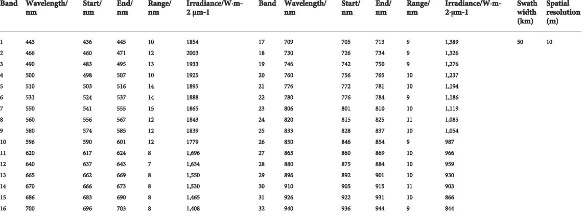
TABLE 1. OHS-3A CMOS1 hyperspectral sensor parameters.
To perform cloud detection, the image must be radiometrically calibrated first to change from a digital number (DN) to radiance as follows:
where L is the radiance in
where
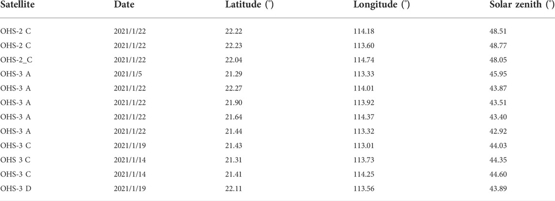
TABLE 2. OHS candidate image information.
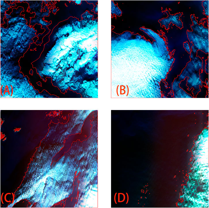
FIGURE 1. Hyperspectral image of the cloud detection (false Color Composite image of bands 26, 13, 6 in RGB, the red vector is the visually interpreted cloud boundary). Image acquisition date (A) 2021/1/5; (B) 2021/1/22; (C) 2021/1/19; (D) 2021/1/14).
The OHS image has 32 bands with a strong correlation between bands and a large amount of redundant information. Meanwhile, some studies have noted that up to 90% of the spectral bands are unnecessary without affecting the overall information decoding accuracy (Chang, 2007). Therefore, before the work of cloud detection, the hyperspectral images’ dimensions must be approximately reduced to reduce the redundant information and retain the valuable information. We use principal component analysis (PCA) (Abdi and Williams, 2010) to extract the first three principal components of the image. The new image contains most of the features of the previous data and effectively removes most of the noise while having a lower dimensionality for subsequent processing.
The pixels of each OHS image are approximately 5050*5050. To input the remote sensing images into the deep neural network for efficient training, the images must be sliced and processed, and the remote sensing images are sequentially sliced into 512*512 sizes. Therefore, each OHS image can be sliced into 81 pieces of 512*512 pixel size. In this study, 972 sample data are obtained in total, and the subsequent neural network training and validation samples are divided using a 4:1 ratio.
U-Net is a convolutional neural network architecture that was first used for biomedical image segmentation (Ronneberger et al., 2015). U-Net is a U-shaped encoder-decoder network architecture that consists of four encoder blocks and four decoder blocks, which are connected via a bridge. The spatial dimension of the encoder network (contracting path) is half, and the number of filters (feature channels) for each encoder block is doubled. The encoder network acts as a feature extractor to learn the abstract representation of the input image through a sequence of encoder blocks. The encoder consists of convolutional and maximum pooling layers to extract features from the image. The decoder network is used to take the abstract representation and generate a semantic segmentation mask. The decoder uses up-sampling to recover the original resolution of the input by transposed convolution. The last decoder gives a segmentation mask, which represents the pixel-level classification using a sigmoid activation function. The encoder and decoder paths are connected by a convolution layer for feature fusion. The U-Net structure allows efficient access to the contextual and location information. Since U-Net has a very similar backbone network to VGG16 and ResNet50, we imported the U-Net model into VGG16 and ResNet50 as the backbone network and loaded the weights of image nets in the subsequent transfer learning process.
VGG is a widely used convolutional neural network architecture proposed by Karen Simonyan and Andrew Zisserman from the University of Oxford (Simonyan and Zisserman, 2014). The architecture of VGG comprises eight layers in total, the first five of which are convolutional layers, the last three are fully connected layers, and all outputs of the convolutional and fully connected layers are connected to the ReLu nonlinear activation function. The entire network uses the same-size convolutional kernel size (3 × 3) and max-pooling size (2 × 2). VGG uses multiple convolutional layers with smaller convolutional kernels (3 × 3) instead of a convolutional layer with a larger convolutional kernel, which reduces the parameters while improving the model fitting ability by continuously deepening the network architecture.
With the complexity of the network architecture, there is a decrease in accuracy of the training set, which can be determined not to be due to overfitting (the training set should be highly accurate in the case of overfitting). When the depth of the neural network is deeper, it may not have a good effect like the shallow model training due to the gradient disappearance or gradient explosion generated during the network training. A completely new network, which is called the deep residual network (ResNet) (He et al., 2016), has been proposed to address this problem and allows training deeper networks. ResNet uses residual blocks to improve the model accuracy. At the core of the residual blocks is the concept of “skipped connections,” which is the strength of ResNet. ResNet-50 is a 50-layer-deep convolutional neural network. Compared to VGGNets, ResNets are less complex because they have fewer filters.
In transfer learning, we use a strategy called fine-tuning, which allows a portion of the pre-trained layers to be retrained. We use pre-trained layers of VGG16 and ResNet-50 to extract features. There is no actual training on these pre-trained layers. We freeze the pre-trained convolutional layers and unfreeze the last few pre-trained layers for training. The frozen pre-trained layers will be convolved with visual features as usual. The nonfrozen (trainable) pre-trained layers will be trained on our custom dataset and updated based on the predictions of the fully connected layers. The network fine-tuning adjusts the parameters of the trained network to the new task at hand. The initial layers learn very general features, and as deeper network layers are introduced, the layers tend to learn more specific task patterns. Therefore, to fine-tune, we keep the initial layers intact (or freeze) and retrain the later layers for our task.
In the training process of the cloud detection model, the U-Net backbone network is selected to freeze the first 16 layers when using the pre-training weights file of VGG16; for ResNet50, the first 150 layers are frozen. For the newly added cloud sample data, 20 generations are trained, where the first 10 generations are frozen and the last 10 generations are trained using the full layers to ensure that the new cloud detection model can have a strong generality.
The flowchart of cloud detection is shown in Figure 2. First, the hyperspectral images are first calculated from DN values to apparent reflectance. Then, the first three principal components are extracted using PCA, the clouds are distinguished from clear sky pixels using visual interpretation, and the original images are sliced to produce training samples. Afterwards, the U-Net structure is used, and transfer learning is performed using pre-trained VGG16 and ResNet50 to obtain end-to-end network models and classification results for each pixel. Because clouds generally appear on a large scale and in successive pieces, for discrete image elements that are determined as clouds, clump is performed, i.e., if fewer than 5 successive pixels in the range of 3*3 pixels are determined as clouds, all pixels are re-determined as clear sky pixels.
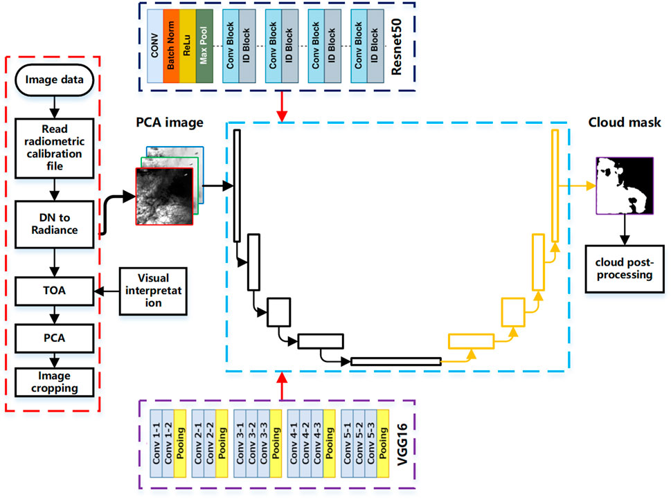
FIGURE 2. Cloud detection algorithm flow chart.
To validate the detection results of the model, two types of accuracy metrics are used for evaluation: the overall accuracy (OA) and F1 score. The OA is the probability that for each random sample, the classified result matches the true data type, and the F1 score is an overall measure of the model accuracy, combining recall and precision. For these two metrics, a higher score indicates a higher-quality algorithm.
where
Figure 3 shows the cloud detection results of the algorithm in this paper compared with the visual interpretation results, and the red curve in the figure is the edge of the cloud region for visual interpretation. The first row is the original image, the second row is the detection result using VGG16 as the backbone, and the third row is the detection result using ResNet50 as the backbone.
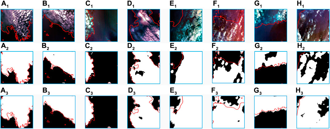
FIGURE 3. Cloud detection results, in which white is the cloud pixels, black is the clear sky pixels, and the red curve is the visually interpreted cloud boundary. The first row is the original image, the second row is the result based on the VGG weights detection, and the third row is the result using the Resnet50 weights detection. (A–H) are slice images with a size of 512*512.
Table 3 shows the detection statistics of the eight images. The detection results using ResNet50 as the backbone network are much closer to the visual interpretation; the average overall accuracy is 86% and 91.8% with VGG16 and ResNet50 as the backbone network, respectively. Meanwhile, both have extremely similar F1 values (approximately 78%). For the full validation data, the overall accuracy of VGG16 is 87.1%, and the overall accuracy of ResNet50 is 90.1%. From the graph of detection results and statistical results, VGG16 has smaller detection result values than ResNet50. Analyzing all data, we find that the detection results of VGG16 are completely included in Resnet50, and Resnet50 has a better overall detection accuracy than VGG16 in terms of the visual interpretation results.
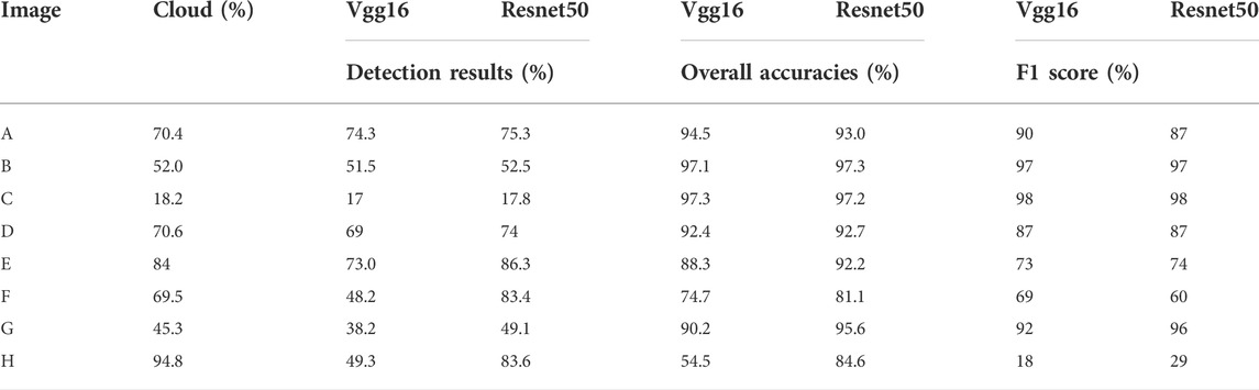
TABLE 3. Statistics of cloud detection accuracy.
For the misjudgment of the thin cloud region, the visual interpretation results are compared with the detection results of VGG and Resnet50, and the TOA reflectance is counted, as shown in Figure 4. The blue color among the three lines is the spectral curve of the clear sky pixels, red indicates the cloud pixels that are classified as cloud pixels by all models, and green indicates that only Resnet50 detects as cloud pixels. In the wavelength range of 600–940 nm, the difference between the three models is very small, and the TOA reflectance is basically identical. In the range of 440–470 nm, the clear sky pixels have the lowest TOA reflectance. In the wavelength range of 480–580 nm, the cloud pixels have higher TOA reflectance than the clear sky pixels. This is most likely because the lower surface of the cloud pixels is water, which is visually very close to the shadows and are identified as cloud pixels in the visual interpretation due to the surrounding cloud pixels. Meanwhile, in some images with a high percentage of thick clouds, if there is a mostly small area of broken clouds, there is a very small gap between neighboring clouds. In the visual interpretation process, there is no obvious boundary between the ground and thin clouds, and there is a certain degree of subjectivity in the interpretation, which will affect the verification results and decrease the accuracy.
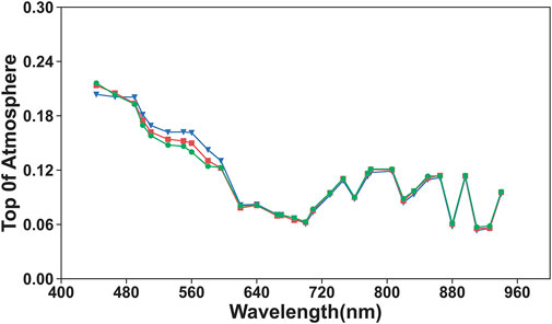
FIGURE 4. Comparison of the TOA reflectance curves. Blue is clear sky pixels, red is visually interpreted as clear sky pixels that are classified as cloud pixels by all models, and green is identified as cloud pixels by only Resenet50.
In this study, some remaining problems must be improved or discussed. In the process of transfer learning and fine-tuning the network using pre-trained weight files, the shallow part of the feature extraction network is frozen, and the higher-level features are updated using the target data to fine-tune the network parameters, but the change in number of frozen layers affects the model results, and the optimal allocation between the number of frozen layers and the resource overhead must be further discussed. Meanwhile, the input data of the deep learning model are the first three principal components after PCA operation. There are obvious differences in values compared with the original data, which needs further discussion and verification of whether higher accuracy can be achieved by using different band combinations of the original data. The subjective nature of visual interpretation may also cause differences between the training samples and the real state of the ground surface, which eventually causes misjudgment of the detection results. When the underlying surface is water, a large amount of vapor is produced, which is also judged as clouds in the visual interpretation. Water vapor also obscures the underlying surface, causing the absence of surface features, so there is also a need to discuss whether water vapor over water bodies needs to be detected separately. At present, there are more public data for cloud detection of remote sensing images, but these samples are mainly multi-spectral remote sensing images. In the future, we will establish a standard dataset for a wider range and a longer time scale and acquire hyperspectral images of different latitudes, longitudes and times around the world to verify and compare based on the unified samples. This effort will be more judicious for the accuracy of the detection results of different algorithms and more conducive to the generalization research of the model. In addition, shadows in remote sensing images can obscure ground information and cause the same effect as cloud pixels, and the corresponding detection will be performed for cloud shadows in future research.
The “Zhuhai-1” hyperspectral satellite has 32 bands of data in the visible and near-infrared wavelength range (400–1,000 nm). In this paper, according to the characteristics of OHS hyperspectral data, the first three principal components are extracted using the principal transformation method to remove data noise and reduce the data dimensionality. Based on the transfer learning method, using the U-Net framework, the encoder uses pre-trained VGG16 and ResNet50 models while freezing the bottom features. For the top features, we use the visually decoded cloud image element samples for update training through the fine-tuning of the weights. Finally, we realize the automatic detection of cloud pixels. In the case of small sample training data, the use of the transfer learning method can obtain a cloud detection model with stronger generalization ability through a smaller training cost. In the accuracy verification of this paper, using Resnet50 as the backbone network can lead to an overall accuracy of detection of 91%, and it can also achieve effective detection for thin cloud regions.
The original contributions presented in the study are included in the article/supplementary material, further inquiries can be directed to the corresponding author.
WJ conducted the analysis, writing, and formulation of the idea. WY, WW, SH, and SL supported the formulation of the idea and provided comments on the content of the paper.
This research was funded by the National Natural Science Foundation of China (NO. 42101362, 31501225); the Natural Science Foundation of Henan Province of China (NO. 222300420463).
WY is employed by Geovis Technology Co., Ltd. WW is employed by Zhuhai Orbita Aerospace Science and Technology Co., Ltd.
The remaining authors declare that the research was conducted in the absence of any commercial or financial relationships that could be construed as a potential conflict of interest.
All claims expressed in this article are solely those of the authors and do not necessarily represent those of their affiliated organizations, or those of the publisher, the editors and the reviewers. Any product that may be evaluated in this article, or claim that may be made by its manufacturer, is not guaranteed or endorsed by the publisher.
Abdi, H., and Williams, L. J. (2010). Principal component analysis. WIREs. Comp. Stat. 2 (4), 433–459. doi:10.1002/wics.101
Chang, C-I. (2007). Hyperspectral data exploitation: theory and applications. USA: John Wiley & Sons.
Fischer, T., and Krauss, C. (2018). Deep learning with long short-term memory networks for financial market predictions. Eur. J. Oper. Res. 270 (2), 654–669. doi:10.1016/j.ejor.2017.11.054
Fu, H., Shen, Y., Liu, J., He, G., Chen, J., Liu, P., et al. (2018). Cloud detection for FY meteorology satellite based on ensemble thresholds and random forests approach. Remote Sens. (Basel). 11 (1), 44. doi:10.3390/rs11010044
Ghasemian, N., and Akhoondzadeh, M. (2018). Introducing two Random Forest based methods for cloud detection in remote sensing images. Adv. Space Res. 62 (2), 288–303. doi:10.1016/j.asr.2018.04.030
Ghassemi, S., and Magli, E. (2019). Convolutional neural networks for on-board cloud screening. Remote Sens. (Basel). 11 (12), 1417. doi:10.3390/rs11121417
Giuffrida, G., Diana, L., De Gioia, F., Benelli, G., Meoni, G., Donati, M., et al. (2020). Cloudscout: a deep neural network for on-board cloud detection on hyperspectral images. Remote Sens. (Basel). 12 (14), 2205. doi:10.3390/rs12142205
He, K., Zhang, X., Ren, S., and Sun, J. (2016). “Deep residual learning for image recognition,” in 2016 IEEE Conference on Computer Vision and Pattern Recognition (CVPR)Las vegas,USA, 27-30 June 2016, 770–778.
Jang, J. D., Viau, A. A., Anctil, F., and Bartholomé, E. (2006). Neural network application for cloud detection in SPOT VEGETATION images. Int. J. Remote Sens. 27 (4), 719–736. doi:10.1080/01431160500106892
Ji, S., Dai, P., Lu, M., and Zhang, Y. (2020). Simultaneous cloud detection and removal from bitemporal remote sensing images using cascade convolutional neural networks. IEEE Trans. Geosci. Remote Sens. 59 (1), 732–748. doi:10.1109/tgrs.2020.2994349
Jiang, Y., Wang, J., Zhang, L., Zhang, G., Li, X., and Wu, J. (2019). Geometric processing and accuracy verification of Zhuhai-1 hyperspectral satellites. Remote Sens. (Basel). 11 (9), 996. doi:10.3390/rs11090996
Joshi, P. P., Wynne, R. H., and Thomas, V. a. (2019). Cloud detection algorithm using SVM with SWIR2 and tasseled cap applied to Landsat 8. Int. J. Appl. Earth Obs. Geoinf. 82, 101898. doi:10.1016/j.jag.2019.101898
Krizhevsky, A., Sutskever, I., and Hinton, G. E. (2012). Imagenet classification with deep convolutional neural networks. Adv. Neural Inf. Process. Syst. 25. doi:10.1145/3065386
Lecun, Y., Bengio, Y., and Hinton, G. (2015). Deep learning. Nature 521 (7553), 436–444. doi:10.1038/nature14539
Mateo-García, G., Gómez-Chova, L., Amorós-López, J., Muñoz-Marí, J., and Camps-Valls, G. (2018). Multitemporal cloud masking in the google Earth engine. Remote Sens. (Basel). 10 (7), 1079. doi:10.3390/rs10071079
Pantazi, X. E., Moshou, D., Alexandridis, T., Whetton, R. L., and Mouazen, A. M. (2016). Wheat yield prediction using machine learning and advanced sensing techniques. Comput. Electron. Agric. 121, 57–65. doi:10.1016/j.compag.2015.11.018
Qiu, S., He, B., Zhu, Z., Liao, Z., and Quan, X. (2017). Improving Fmask cloud and cloud shadow detection in mountainous area for Landsats 4–8 images. Remote Sens. Environ. 199, 107–119. doi:10.1016/j.rse.2017.07.002
Qiu, S., Zhu, Z., and Woodcock, C. E. (2020). Cirrus clouds that adversely affect landsat 8 images: what are they and how to detect them? Remote Sens. Environ. 246, 111884. doi:10.1016/j.rse.2020.111884
Ronneberger, O., Fischer, P., and Brox, T. (2015). U-net: Convolutional networks for biomedical image segmentation. Germany: Springer, 234–241.
Schmidhuber, J. (2015). Deep learning in neural networks: An overview. Neural Netw. 61, 85–117. doi:10.1016/j.neunet.2014.09.003
Shendryk, Y., Rist, Y., Ticehurst, C., and Thorburn, P. (2019). Deep learning for multi-modal classification of cloud, shadow and land cover scenes in PlanetScope and Sentinel-2 imagery. ISPRS J. Photogramm. Remote Sens. 157, 124–136. doi:10.1016/j.isprsjprs.2019.08.018
Simonyan, K., and Zisserman, A. (2014). Very deep convolutional networks for large-scale image recognition.arxiv
Sun, H., Li, L., Xu, M., Li, Q., and Huang, Z. (2020). Using minimum component and CNN for satellite. Remote Sens. Image Cloud Detect. 18 (12), 2162–2166.
Sun, L., Mi, X., Wei, J., Wang, J., Tian, X., Yu, H., et al. (2017). A cloud detection algorithm-generating method for remote sensing data at visible to short-wave infrared wavelengths. ISPRS J. Photogramm. Remote Sens. 124, 70–88. doi:10.1016/j.isprsjprs.2016.12.005
Sun, L., Wei, J., Wang, J., Mi, X., Guo, Y., Lv, Y., et al. (2016). A universal dynamic threshold cloud detection algorithm (UDTCDA) supported by a prior surface reflectance database. J. Geophys. Res. Atmos. 121 (12), 7172–7196. doi:10.1002/2015jd024722
Sun, L., Yang, X., Jia, S., Jia, C., Wang, Q., Liu, X., et al. (2020). Satellite data cloud detection using deep learning supported by hyperspectral data. Int. J. Remote Sens. 41 (4), 1349–1371. doi:10.1080/01431161.2019.1667548
Taravat, A., Del Frate, F., Cornaro, C., and Vergari, S. (2014). Neural networks and support vector machine algorithms for automatic cloud classification of whole-sky ground-based images. IEEE Geosci. Remote Sens. Lett. 12 (3), 666–670. doi:10.1109/lgrs.2014.2356616
Wei, J., Huang, W., Li, Z., Sun, L., Zhu, X., Yuan, Q., et al. (2020). Cloud detection for Landsat imagery by combining the random forest and superpixels extracted via energy-driven sampling segmentation approaches. Remote Sens. Environ. 248, 112005. doi:10.1016/j.rse.2020.112005
Yuan, Y., and Hu, X. (2015). Bag-of-words and object-based classification for cloud extraction from satellite imagery. IEEE J. Sel. Top. Appl. Earth Obs. Remote Sens. 8 (8), 4197–4205. doi:10.1109/jstars.2015.2431676
Zhai, H., Zhang, H., Zhang, L., and Li, P. (2018). Cloud/shadow detection based on spectral indices for multi/hyperspectral optical remote sensing imagery. ISPRS J. Photogramm. Remote Sens. 144, 235–253. doi:10.1016/j.isprsjprs.2018.07.006
Zhang, Y., Rossow, W. B., Lacis, A. A., Oinas, V., and Mishchenko, M. I. (2004). Calculation of radiative fluxes from the surface to top of atmosphere based on ISCCP and other global data sets: Refinements of the radiative transfer model and the input data. J. Geophys. Res. 109 (D19), D19105. doi:10.1029/2003jd004457
Zhu, Z., Wang, S., and Woodcock, C. E. (2015). Improvement and expansion of the Fmask algorithm: Cloud, cloud shadow, and snow detection for Landsats 4–7, 8, and Sentinel 2 images. Remote Sens. Environ. 159, 269–277. doi:10.1016/j.rse.2014.12.014
Keywords: cloud detection, hyperspectral image, deep learning, Zhuhai-1, U-Net
Citation: Jian W, Yi W, Wenlong W, Lei S and Haiping S (2022) Transfer-learning-based cloud detection for Zhuhai-1 satellite hyperspectral imagery. Front. Environ. Sci. 10:1039249. doi: 10.3389/fenvs.2022.1039249
Received: 07 September 2022; Accepted: 22 September 2022;
Published: 07 October 2022.
Edited by:
Jing Wei, University of Maryland, College Park, United StatesCopyright © 2022 Jian, Yi, Wenlong, Lei and Haiping. This is an open-access article distributed under the terms of the Creative Commons Attribution License (CC BY). The use, distribution or reproduction in other forums is permitted, provided the original author(s) and the copyright owner(s) are credited and that the original publication in this journal is cited, in accordance with accepted academic practice. No use, distribution or reproduction is permitted which does not comply with these terms.
*Correspondence: Wang Jian, d2FuZ2pfcnNAMTI2LmNvbQ==
Disclaimer: All claims expressed in this article are solely those of the authors and do not necessarily represent those of their affiliated organizations, or those of the publisher, the editors and the reviewers. Any product that may be evaluated in this article or claim that may be made by its manufacturer is not guaranteed or endorsed by the publisher.
Research integrity at Frontiers
Learn more about the work of our research integrity team to safeguard the quality of each article we publish.