 Md. Abu Issa Gazi
 Md. Nahiduzzaman
 Jakhongir Shaturaev
 Bablu Kumar Dhar
 Md. Abdul Halim2
95% of researchers rate our articles as excellent or good
Learn more about the work of our research integrity team to safeguard the quality of each article we publish.
Find out more
ORIGINAL RESEARCH article
Front. Environ. Sci. , 28 October 2022
Sec. Environmental Economics and Management
Volume 10 - 2022 | https://doi.org/10.3389/fenvs.2022.1005814
Current literature conveys that in spite of multiple studies being conducted to explore the influences of various macroeconomic factors both geographical and non-geographical on the CO2 emissions in different parts of the world, there is a scarcity of the same analyses from oil-producing countries. In this study, we reveal a new dimension by investigating the dynamic linkage of climate change, economic growth, energy use, and agricultural and rural development to the CO2 emissions of oil-producing countries around the world. In doing so, we apply Pedroni and Kao panel cointegration test, vector error correction model (VECM), pairwise Granger causality test, impulse response function (IRF), and some supportive models such as-generalized method of moments (GMM), and fixed-effect models. Our primary VAR-based models’ evidence that energy use (EUE), foreign direct investment (FDI), and trade to GDP (TPR) rate have both short-run and long-run casual consequences in CO2 emissions, while only long-run Granger causality is running from agricultural land ratio (ALR), forest area ratio (FAR), gross domestic product (GDP), population growth rate (PGR), renewable energy consumption (REC), and rural population rate (RPR) to CO2 emissions. However, bidirectional associations are observed between CO2 to foreign direct investment and trade percentage rate; EUE to renewable energy consumption and TPR; and TPR to FDI and gross domestic product. To demonstrate the significant impact, our secondary analysis tools GMM and fixed-effect regressions’ results disclose that high energy use and more domestic products significantly contaminate the environmental condition by increasing CO2 emissions in the atmosphere. Hence, our research provides great implications for the authorities of government, producers, businessmen, and general public in the oil-producing countries to ensure a sustainable environment by reducing energy use or alternating with renewable energies and emphasizing environmentally friendly products production over the long-run rather than conventional products production in the short-run.
Global climate change is a weighty concern for the current era and has been in an alarming position worldwide. According to the data from the International Energy Agency, global carbon emissions have augmented by 40% since the early 1970s. (IEA, 2013). British petroleum review of statistics for world energy revealed that CO2 emissions have increased by 3729.8 million tons compared to the figure in20091. In 2021, global CO2 emissions increased to their highest level ever, a recent report from IEA evidenced that global energy-related CO2 emissions increased by 6%–36.3 billion tones (IEA, 2022). However, during the COVID-19 pandemic period in 2020, world CO2 emissions slightly decreased (Li & Haneklaus, 2022). Plenty of factors, namely, burning fossil fuels for energy production (Luqman et al., 2019; Paraschiv & Paraschiv, 2020), electricity production (Malla, 2009), oil production (Ike et al., 2020), high crude oil demand (Krantz et al., 2022), industrialization (Sikder et al., 2022), urbanization (Islam et al., 2021), and rural population growth (Gyamfi, 2022), contaminate the global climate by increasing CO2 emissions in the atmosphere. Environmental dilapidation by various types of pollution is a major subject for all the countries around the world (Rogelj et al., 2013; Castán Broto, 2017).
According to the global carbon project from 2020, the United States, China, Russia, Germany, and the United Kingdom are the top five carbon emissions countries followed by other top oil-producing nations-such as Canada, Indonesia, Saudi Arabia, Brazil, Mexico, and Australia (Blokhin, 2022). The ruthless significant impact of crude oil on environmental problems is termed as an imperative strategic resource for economic enhancement that has reached 2239 million tons in 2019 (Wang et al., 2021). In current literature, on the one hand, recent studies (e.g., Oh et al., 2010; Andersson & Karpestam, 2013; Chevallier et al., 2019; Ullah et al., 2020; Alkathery & Chaudhuri, 2021; Wang et al., 2021) investigated the linkage between carbon emissions and crude oil prices, and on the other hand, some other studies (e.g., He et al., 2005; Gavenas et al., 2015; Agboola et al., 2021; Hao et al., 2022; Kassouri et al., 2022) explored the consequences of oil price and extraction on the CO2 emissions. Besides, many studies (e.g., Antweiler et al., 2001; Cole & Elliott, 2003; Azam & Khan, 2017; Hasanov et al., 2018; Ike et al., 2020; Islam et al., 2021; İnal et al., 2022) demonstrated the connection of consumption of renewable energy, economic progress, governing efficiency of energy, electricity production, GDP, international trade, export, import, and urbanization to the carbon dioxide emissions in different countries or specific part of the world community.
Interestingly, there is no shred of evidence about the impact of various macroeconomic factors both geographical and non-geographical on the CO2 emissions in the oil-producing countries. Furthermore, studies expose that the CO2 emissions are drastically increasing in the oil-producing countries and these countries are becoming the top CO2 emissions countries around the world. Islam et al. (2021) stated that economic development, trade volume, and urbanization worsen the environmental superiority by flourishing CO2 emissions, while globalization, FDI, and innovation have favorable effects on the environment. However, globalization as an environmental consequence has been a matter of global debate (Blanco et al., 2013). Pan et al. (2018) depicted that every nation is prioritizing economic progress, although Adom et al. (2018) stated that economic growth challenges environmental sustainability. The unstable oil production plays a significant role in the international economy despite the continued contamination of the global climate. Furthermore, the reduction of CO2 emissions has become an essential segment of the energy and economic policy stratagems of countries globally. Therefore, it is essential to see the impact of various macroeconomic factors like climate change, economic growth, energy use, agriculture and rural development on the CO2 emissions in nations that produce oil.
İnal et al. (2022) established a nexus between renewable energy consumption, economic enhancement, and CO2 discharges in oil-producing countries in Africa. Accordingly, Ebohon and Ikeme (2006) examined the putrefaction impact of CO2 emissions in SSA oil- and non-oil-producing nations. Saidi & Omri, (2020) explored the linkage between CO2 emissions, renewable energy, and nuclear energy in 15 OECD states. They found an important link between energy use, economic progress, and CO2 emissions in these oil-producing regions. Furthermore, according to a report by the Tyndall Centre for Climate Change Research, wealthy economists should stop producing oil and gas by 2034 if they want to keep global warming at 1.5°C2. So, there should have evidence about how much the macroeconomic conditions both geographical and non-geographical affect the carbon dioxide emissions in top oil-producing countries.
Moreover, our research has multiple implications that ramify the clear circumstances of carbon emissions sensitivity, actions, and guidelines for the general people, businessmen, producers, policymakers, and government authorities. However, to the best of our understanding, this is the first study to explore the impact of macroeconomic factors on CO2 emissions in oil-producing countries. Second, to accurately depict the influencers that directly affect CO2 emissions, we take into account a number of factors as proxies and consider 22 top oil-producing countries around the world. Third, from the methodological viewpoint, we apply the vector error correction model (VECM) that can captures the long-term and short-term causal associations between the dependent and independent variables along with the directional relationship between the variables. In addition, we also use generalized method of moments (GMM), and fixed effect models to reveal the significant relationship between the dependent and independent variables. Finally, we derive some astute recommendations for developing the sustainability of the environment in the researched regions based on the study’s findings.
Using VECM, our empirical findings show that on the one hand, only long-run Granger causality is running from ALR, FAR, GDP, PGR, REC, and RPR to CO2 emissions, and on the other hand, both short- and long-term causal effect are running from EUE, FDI, and TPR to CO2 emissions. The directional relationship approach, pairwise Granger causality test, evidences CO2, TPR, REC, EUE, TPR, and GDP have bidirectional relationship with FDI, CO2, EUE, TPR, FDI, and TPR respectively. The GMM and OLS techniques unveil that EUE and GDP positively and significantly impact the CO2 emissions in oil-producer countries.
The remaining parts of the paper are ordered as follows: The previous studies relevant to our paper are represented in Section 2. Section 3 demonstrates the data sources and methodological details. The empirical findings are displayed and expounded in Section 4. Finally, Section 5 exhibits the concluding remarks.
The subject of connection between energy use and production, economic growth, renewable energy consumption, export and import, globalization, urbanization, industrialization, deforestation and carbon dioxide emissions has been well documented in the existing literature. Different researchers consider different countries, continents, nations at different economic organizations in different time frames to investigate the association of various external and internal factors with the CO2 emissions. Furthermore, many academics and decision-makers have recently focused on the connection between climate change, energy use, and sustainable economic growth (Salari et al., 2021). In the atmosphere, CO2 emissions are largely influenced by energy use, economic growth, trade and urbanization (Kasman & Duman, 2015). The industrial revolution is marked the beginning of the largest human-caused impact to climate changes, as burning fossil fuels such as-gas, coal, and oil boosted atmospheric concentrations of greenhouse gases (IPCC, 2007). Anser et al. (2020) stated that for ensuring the balance between economic, environmental, and social aspects, adapting with atmospheric change is considered as an important component. However, we properly look out the past studies associated to CO2 emissions that are demonstrated in the beneath level.
In order to understand how economic development is governed by renewable energy and CO2 emissions in Africa’s oil-producing regions, İnal et al. (2022) looked at the general relationship between renewable energy consumption, CO2 emissions, and economic development. They found from the AGM estimation that CO2 emissions do not boost the progress of the economy in the overall panel along with an insignificant relationship of economic growth to renewable energy consumption. Furthermore, Ebohon & Ikeme (2006) investigated the decomposition role of CO2 emissions predominance and the use of energy severity in CO2 emissions in the sub-Saharan African (SSA) oil- and non-oil producing nations by Laspeyres decomposition model. Their major findings implied that switching high carbon acute energy to low carbon acute energy can diminish the adverse movement of CO2 emissions. In that same geographical area, Sarpong & Bein (2020) explored the effect of good corporate governance on CO2 emissions. Oil-producing regions have good corporate governance that regimens and lessens the CO2 emissions (Abid, 2016; Hassan et al., 2020; Sarpong & Bein, 2020; Sinha & Shahbaz, 2018. Correspondingly, Azam & Khan (2017); Ibitoye and Akinbami, (1999) emphasized energy use reduction, developing the governing efficiency of energy, shifting to the low carbon concentrated fuels, flourishing the renewable energy consumption, and reducing the gas flare can change the magnitude of CO2 emissions. The severity of CO2 emissions, demand for oil, and military potency are largely connected to each other in China and India over the long-run period reported by (K. H. Wang et al., 2021). K. H. Wang et al. (2021) inspected whether the crude oil dependency and CO2 emissions affect the military expenses in oil-importing nations. Also, Lindstad & Eskeland (2016); Lindstad et al. (2015), (2020) interconnected the maritime industry with CO2 emissions.
Alkathery & Chaudhuri (2021) found the explosive spillover upshot and co-movement among crude oil price, CO2 emissions, and worldwide fresh energy production. Subsequently, Krantz et al. (2022) expressed that low demand for oil-related products enhances the environmental condition by reducing CO2 emissions. Specifically, high crude oil demand contributes a momentous role in worsening the condition of CO2 emissions that they have found. Using the MMQR model along with fixed effects, Ike et al. (2020) evaluated the interrelatedness between oil production, CO2 emissions, electricity production, GDP, trade, and democracy in 15 oil-producer nations over the year 1980–2010. The outcomes showed that oil and electricity production are liable to intensify the CO2 emissions whereas trade volume diminishes environmental pollution. Initially, Antweiler et al. (2001); Cole & Elliott (2003) investigated the impact of international trade on environmental degradation. In African OPEC countries, the interconnectedness between carbon dioxide (CO2), nitrous oxide, methane with growth of the economy and energy consumption are evaluated by (Yusuf et al., 2020). Yusuf et al. (2020) used carbon dioxide (CO2), nitrous oxide, methane as proxies for greenhouse gas that can degrade the environment. Gyamfi (2022) conducted a study on consumption-based carbon emissions in SSA nations that produce oil. A well-adjusted panel econometrics analysis along with AMG, CCEMG, DK OLS methods are used in this study where investigation results demonstrated that rural population growth, FDI, natural resources, and income positively affect the ecological quality, namely, the consumption-based CO2 emersions. In the same direction Hasanov et al. (2018) explored the impact of GDP, export, and import factors on the CO2 emissions based on consumptions in oil-exporting countries. The findings uncovered that GDP and imports enhance the ecological environment; however, exports play a ruffle role to contaminate the atmosphere.
Applying VECM and FMOLS Saidi & Omri, (2020) tried to find out the linkage among CO2 emission, atomic energy, and renewable energy in 15 OECD regions. The outcomes of this study explored both atomic energy and renewable energy consumptions improve the environmental condition by reducing carbon emissions. In BRICS countries Hassan et al. (2020a) examined the reliability of atomic energy results on CO2 emissions and found favorable results. To some extent, Alataş (2022) explored the association of the transport sector and environmental technologies with the CO2 emissions in 15 EU countries over the years 1977–2015. The findings attributed that environmentally friendly technologies have a positive but insignificant relationship with CO2 emissions from the viewpoint of transport sector. Furthermore, carbon dioxide eructation is amplified by burning fossil fuels due to energy production (Paraschiv & Paraschiv, 2020), CO2 emissions connectedness with renewable energy shares in energy production (Albulescu et al., 2020), nexus among CO2 emissions, growth of the economy, and consumption of renewable energy (Bilan et al., 2019; Radmehr et al., 2021), the connection of resource charge, using of renewable-nonrenewable energy with CO2 emissions (Bekun et al., 2019), the influence of population on CO2 emissions (Martínez-Zarzoso et al., 2007), the impact of internet usage and progression of economy on CO2 emissions (Salahuddin et al., 2016) are brought to light. Besides that, Mahdi Ziaei (2015) investigated the impact of stock and credit market shocks on CO2 emissions, and energy consumption in EU, East Asian, and Oceanian states. Applying the ARDL approach along with the VAR model Zubair et al. (2020) inquired about the effect of various economic factors like GDI, trade incorporation, inflows of FDI, GDP, and capital on the CO2 emissions in Nigeria. They reported that CO2 emissions have a long-term association with the studied variables where inflows of FDI, fixed capital, and GDP negatively affect the CO2 emissions, however, CO2 emissions have a bidirectional relationship with inflows of FDI along with a unidirectional relationship with capital.
In Addition, Malla (2009) determined the character of the production of electricity, the structure of electricity generation, and the intensity of energy for electricity generation on CO2 emissions in the most electricity generated countries such as- Korea, India, Australia, United States , Japan, Canada, and China. The author’s findings demonstrated that electricity production is forecasted to be the key factor for increasing the CO2 emissions till in 2030, while the intensity of energy effect in electricity production could decrease the emissions. However, Sheinbaum et al. (2011) stated due to the heavy dependability on fossil fuels, the reduction of energy intensity did not significantly decrease the CO2 emissions in Argentina, Brazil, Colombia, and Mexico. Using Granger causality test method, Blanco et al. (2013) investigated the upshots of FDI from various points of view on CO2 emissions in 18 Latin American regions and originated a causal relationship running from the FDI in profanation exhaustive industries to CO2 emissions.
Tiwari & Mishra (2016) tested the convergence of CO2 emissions in 18 Asian countries by applying parametric and non-parametric tests and showed the convergence of CO2 emissions is significant in the recent decades where per capita emissions play a vital role in projection of the CO2 emissions. Employing the STIRPAT model, Khan et al. (2018) inspected the encouragement of financial enhancement, unevenness of income, and GDP on emissions of carbon dioxide in south Asian countries. Their results indicated that income inequality reduces the CO2 emissions in India and Pakistan but increases the same in Bangladesh, while financial enhancement develops the ecological circumstances in these countries. Islam et al. (2021) studied how the mounting interdependence of the world economy as globalization, FDI, and use of energy affect the CO2 emissions in Bangladesh by dynamic ARDL method. They tried to explore the relation of institutional quality to CO2 emissions. The outcomes found that globalization, FDI, and trademark application as innovation enhance the environmental condition by reducing carbon emissions both in the short- and long-run, whereas growth of the economy, percentage of trade volume in terms of GDP, urbanization, and consumption of energy deteriorate the environment. A similar study was conducted in Pakistan by (M. K. Khan et al., 2019), who found the same results as (Islam et al., 2021) with the exception that energy consumption affects the CO2 emissions positively and innovation affects it inversely. Accordingly, in Malaysia, Philip et al. (2022) observed that renewable energy, technological innovations, and entrepreneur activities reduce the CO2 emissions. Furthermore, using both symmetric (DOLS) and asymmetric (NARDL) methods, Udemba et al. (2022) found the same findings in Turkey. However, fossil fuels contaminate the environment significantly in Brazil (Udemba & Tosun, 2022).
In sum, we may draw conclusions regarding the previous studies on various factors that affect carbon emissions around the world, and at the same time, we find some potential research gaps. First of all, researchers unfolded the sensitivity of carbon emissions considering the particular country, organizational groups, oil-producing countries in a specific continent, and selected countries in a definite continent, whereas the current top oil-producing countries in the world did not consider. Secondly, the effect of esteem and renewable energy consumption, electricity generation, globalization, GDP per capita, FDI, dependence on fossil fuels, economic growth, innovation, maritime industry, transportation, and corporate governance on carbon dioxide emissions are revealed in the above geographical regions. However, the nexus between forest area ratio, population growth, economic enhancement, agricultural and rural development, energy use both esteem and renewable, and CO2 emissions remain unclear in the studied above geographical regions, and particularly there is no such evidence in the top oil-producing countries. Finally, evidence shows that previous studies link short of variables with the CO2 emissions in a single study, where revealing the clear picture of CO2 emissions could be developed by adding some more important variables that have close relationship with CO2 emissions.
This study is based on secondary data, we collect raw data for our research from the world bank database. Besides, for proper evaluation of the past research and current implications of this paper, we collect numerous information from various journals, newspapers, reports, magazines, and websites. Basically, we consider 22 oil-producing countries among the all oil-producing countries around the world depending on the top position and availability of required data in the database file in the world bank. We eliminate Qatar and Kuwait from our sample list because of the insufficiency of data, although they are top position holders as oil producer countries. This study envisages yearly data that covers the study year from 1990 to 2018. The main intuition behind this study is to explore the role of climate change, economic growth, use of energy, agriculture and rural development on the CO2 emissions in oil-producing countries. For those instances, carbon dioxide emissions (CO2) is taken as a dependent variable, and population growth rate (PGR), forest area ratio (FAR) as proxied for climate change; foreign direct investment (FDI), trade percentage rate (TPR), gross domestic product (GDP) as proxied for economic growth; energy use (EUE), renewable energy consumption (REC) as proxied for energy use; and agricultural land ratio (ALR), rural population rate (RPR) as proxied for agriculture and rural development are considered as independent variables. The theoretical framework is represented in Table 1 where title variables along with each variable and its measurement unit are properly demonstrated.
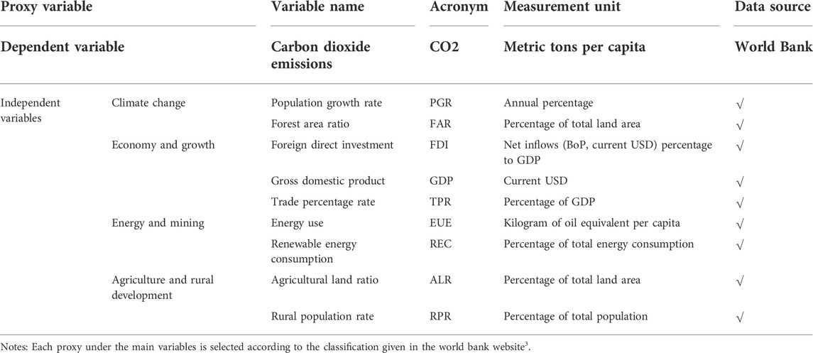
TABLE 1. Theoretical framework.
The general state of the analyzed variables during the course of the study periods is depicted graphically in Figure 1. We see that FAR and RPR follow the downward trend that implies forest area in terms of total land area and rural population to total population rate are drastically falling in every year. However, ALR, EUE, GDP, and TPR got the upward trend in the recent periods. In oil producing nations, oil production plays as a role of driving force behind the change of climate along with enhancing economic growth, trade, globalization, and searching new place for agricultural purpose, dwelling place, and infrastructural development diversifications. Additionally, income increases lead to boost in demand for manufactured items, which forces producers to utilize more energy to keep up with the change in needs in these regions. However, FDI volume decreased in 2017 and 2018 compared to previous few years. According to the United Nations Conference on Trade and Development, due to the 22% decrease in the value of cross-border mergers and acquisitions (M&As), global FDI volume decreased sharply in 2017 and prospects of FDI was still muted in 2018 (UNCTAD, 2018). The CO2 emissions in oil-producing countries increased at the initial period of the study, then, it followed a downward trend till 2000, afterwards CO2 emissions gradually increased till 2008. It is surprising to see that after upward movement, CO2 emissions and PGR are steadily diminishing. We notice that REC slowly decreased in each year till 2014, after a gap it follows the same direction and dies off.
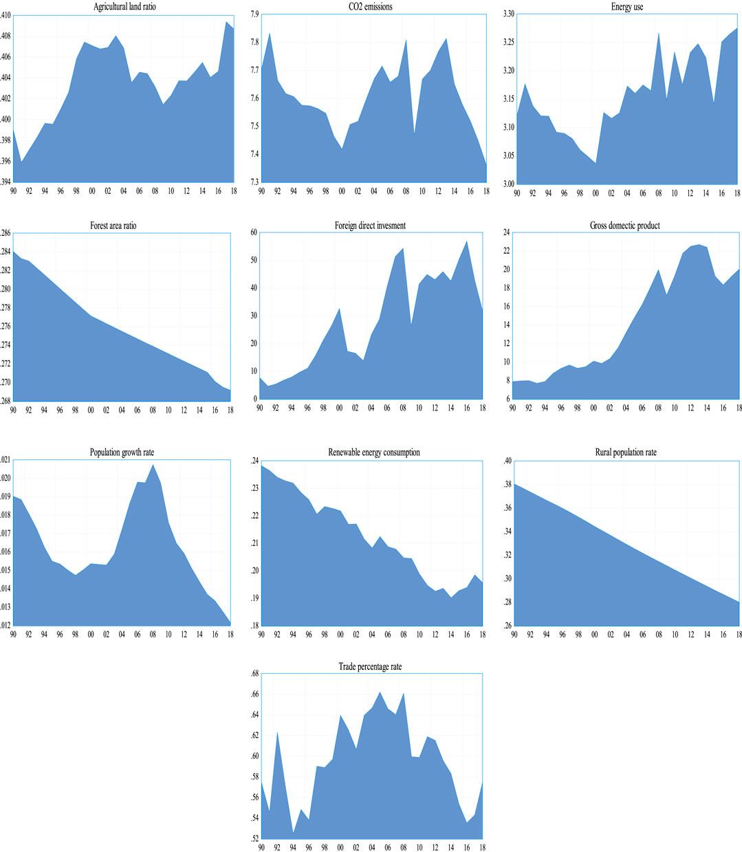
FIGURE 1. Graphical plots of studied variables. Notes: The horizontal axis of each variable indicates the year, e.g., 1990,1991 … … 2018. The vertical axis of each variable denotes the respective raw data, e.g., percentage of total land area in case of agricultural land ratio, metric tons per capita in case of CO2 emissions, kilogram of oil equivalent per capita in case of energy use, and so on.
For proper evaluation the condition of CO2 emissions in oil-producing countries, we apply plenty of techniques like, in case of test the stationarity of data, Levin, Lin & Chu and Breitung unit root tests are used. For evaluating the presence of long-run and short-run relationship between the variables Pedroni and Kao panel cointegration methods are used. Accordingly, by adopting the VAR type models, namely, VECM, and Granger causality (Granger, 1969) test, we explore the short-run and long-run relationship between explanatory variables and dependent variable, and pairwise Granger causality between the variables respectively. Finally, we apply OLS type models such as-GMM (Hansen, 1982) along with fixed-effect model to reveal the significant relationship between the dependent variable and independent variables. However, the used statistical models in this study are thoroughly explained below:
This study considers time-series panel data over the year from 1990 to 2018. We initially demonstrate our mathematical model in simple regression form.
Here,
We convert the root level data to simple logarithm form thus, the model will be:
Unit root test is crucial in determining whether time series or panel variables are stationary. A variable’s unit root content can be assessed using the unit root test in statistics. According to the results of the unit root test, researchers select their research model to evaluate the time series and panel data, otherwise the regression results of data explore spurious results (Danish et al., 2018). According to the rule of thumb, acceptance of null hypothesis (
The results of the unit root test demonstrate that the panel data are non-stationary at level I (0), however, the stationarity issues in each variable are resolved at the first difference I (1), the results are shown in Table 3 that directs to explore the presence of the long- and short-term effect among the variables. According to Al-mulali (2012), as our data have stationary at first difference, we can proceed to test the panel cointegration for rummaging the long- and short-run nexus between the dependent and independent variables. Accordingly, we apply the Pedroni panel cointegration test (Pedroni, 1999) and Kao panel cointegration test (Kao, 1999) to explore the entity of long-term effect within our variables. The rule of Pedroni and Kao cointegration test demonstrates that if the null hypothesis of cointegration
In Pedroni’s panel cointegration test, seven statistics are categorized into two different sections such as-group mean statistics and panel test statistics. Group mean statistics estimate the average outcomes of individual nation test statistics, while panel statistics assemblage the statistics considering the within-dimension. Addressing simple cross-sectional reliance, these tests can comprise the common time dummies that are employed by the time disparaging the data for individual and variables in the manner described below (Neal, 2014):
Since the test statistics are based on residuals, so these residuals are gathered from the beneath regressions:
Where, i = 1, 2, 3, … … …. N indicates the number of countries in the panel, t = 1, 2, 3, … …. T denotes the number of periods, m = 1, 2, 3, … …., M represents the number of regressions, k = 1, 2, 3, … … … , K assigns the number of lags in the ADF regressions. In case of user’s route, trend of linear time
The Engle and Granger type tests are essentially used in the Pedroni and Kao panel cointegration approaches that estimate whether the calculated error term
The distinction between the Pedroni and Kao approaches is that Pedroni method consents the coefficient slope to differ diagonally the members of panel, whilst the Kao statistic invisages homogenous
As our panel data’s variables are cointegrated (results shown in Tables 4, 5), we can use the VECM approach to test the association of dependent variable with the independent variables both in short- and long-run period. VECM approach is compatible at the time of prolonged cointegration between the variables (Pachiyappan et al., 2021). This model also evaluates the pairwise Granger causation between the two variables. We propose the following VECM equation to explore the time wise and pairwise relationship among the explanatory variables including the dependent variable. To apply the test, we propose the following model as the VECM approach.
Here,
Here, c= (
It is possible to rewrite the vector error correction model (VECM) in the manner shown below:
Here,
After detecting the long- and short-run alignment of explanatory variables with the carbon dioxide emissions, we also use GMM statistical method to explore the general significant nexus between independent variables and the dependent variable. GMM pathway is a semiparametric model that controls heteroskedasticity sources of data (Le et al., 2016). GMM model is useful to adjust the problem of maximum likelihood estimator at cointegration. This statistic also helps to test the robustness of our VECM based impulse response function (IRF) outcomes. The GMM model considers an OLS linear regression model. The GMM model equation is specified as follows:
Here,
Table 2 represents summary overviews of the macroeconomic conditions and CO2 emissions in oil-producing countries since 1990 to 2018. We do not present logarithm data, here the table’s indicated unit is used to organize the raw data. The average value of CO2 emissions, FDI and GDP is 7.6112 metric tons per capita, 28.4305 crores and 14.2813 thousand respectively along with high standard deviation. In contrast, the average value of ALR, EUE, FAR, PGR, REC, RPR and TPR is 40.37%, 3.1587 thousand, 27.61%, 1.64%, 21.25%, 33.01%and 59.66% respectively with comparatively lower standard deviation. The variables’ positive skewness values indicate long right-hand tail, while high kurtosis values of the variables denote the heavy tails or outliers. Furthermore, Jarque-Bera statistical results reject
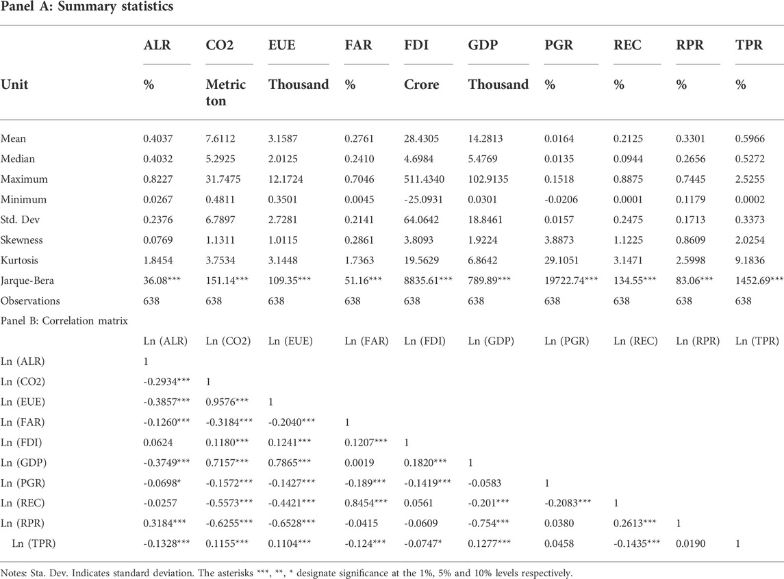
TABLE 2. Summary overviews and correlation.
In the correlation matrix (panel b of Table 2), we observe that each variable is significantly correlated to each other except for ALR association with FDI and REC; FAR linkage with GDP and RPR; FDI relation with REC and RPR; GDP, RPR and TPR familiarity with PGR; and RPR association with TPR. In addition, CO2 emissions have significant positive linkage with EUE, FDI, GDP and TPR, while a significant negative relationship is found between CO2 emissions and ALR, FAR, PGR, REC, and RPR respectively.
Table 3 represents the unit root test results where two methods, namely Levin, Lin & Chu test and Breitung test, are applied to look into the stationarity of the studied variables. We apply the unit root tests on converted raw data into simple logarithm form at first difference. The results indicate that only EUE, FAR and RPR are stationary at level I (0) in Levin, Lin & Chu test, however, none of the variables are stationary at level I (0) in Breitung test because of accepting the null hypothesis at 5% significance level. If we move into the first difference I (1), results show that all of the variables in both tests achieve stationarity as a result of the
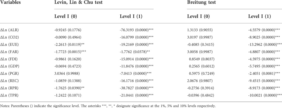
TABLE 3. Panel unit root test.
Table 4, 5 illustrate the outcomes of Pedroni and Kao panel cointegration test where we consider seven statistics, namely, panel v-statistic, panel rho-statistic, panel PP-statistic, panel ADF-statistic, group rho-statistic, group PP-statistic, and group ADF-statistic, in case of Pedroni panel cointegration test, and ADF value in case of Kao panel cointegration test to explore whether the long-run effect presents among our studied variables or not. Moreover, prior to running the cointegration test and creating the VER-based model, it is required to determine the ideal lag length criteria. There is a standard, if the optimal lag length is too small, the cointegration model can explore mis-specified results and accordingly if the optimal lag length is too high, the cointegration model can produce parameterized outcome (Wooldridge, 2009). This study looks at the likelihood ratio (LR), final prediction error (FPE), Akaike’s information criterion (AIC), Schwarz criterion (SC), and Hanna-Quinn (HQ) information criterion value. Among the all criteria, no criterion is preferred over the others although AIC criterion is preferable (Liew, 2004). The lag length selection criterion results are displayed in Table 6. The verdicts show that in case of FPE, AIC criteria optimal lag length is five. However, the ideal lag length, as determined by the SC and HQ criteria, is two. According to Liew (2004), the FPE and AIC criterion lead us to choose a 5 lag as the ideal length. This ideal leg length criterion guides the cointegration test, VER-based model, and Granger pairwise causality link between variables.
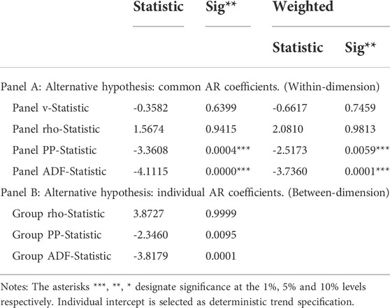
TABLE 4. Pedroni panel cointegration test.
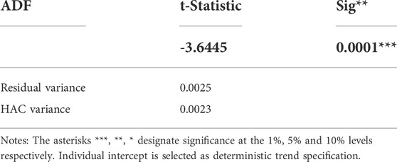
TABLE 5. Kao panel cointegration test.
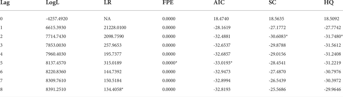
TABLE 6. Results of lag length selection criteria.
The Pedroni panel cointegration results in table 4 are separated in two parts, in the first part panel test statistics are reported and group mean statistics are documented in the second stage. There are total 11 outcomes under 7 hypotheses in the two section including the weighted statistics, among them except the outcomes of panel v-statistic, panel rho-statistic, and group rho-statistic, the six outcomes under the remaining four statistics find rejecting the null hypothesis
Table 7 represents the VECM outcomes that exhibit the time-varying connections between dependent and explanatory variables. The negative coefficient value of ECT at 0.0004 significant level alludes rejecting the null hypothesis that refers there is a long-term causation running from the nine independent variables, namely ALR, EUE, FAR, FDI, GDP, PGR, REC, RPR and TPR, to the dependent variable CO2 emissions. It means that all independent variables have a prolonged impact on the CO2 emissions. To put it another way, from the independent variables to the dependent variable, there is existence of long-term causation. In order to find out the short-run causality between the dependent and independent variable, we convert the value of VECM results at different lagged values of the variables into the single value format by using Wald statistics (Wolfowitz, 1952). The rule of thumb of Wald statistics demonstrates that if the lag variable values are equal to zero representing as accepting the null hypothesis, referring there is no short-run causation running between the respective explanatory variable to the dependent variable (King and Goh, 2002; Yee, 2021). The Wald test statistic results show that there is short-run causal relationship running from the EUE, FDI and TPR to the CO2 emissions as rejecting the
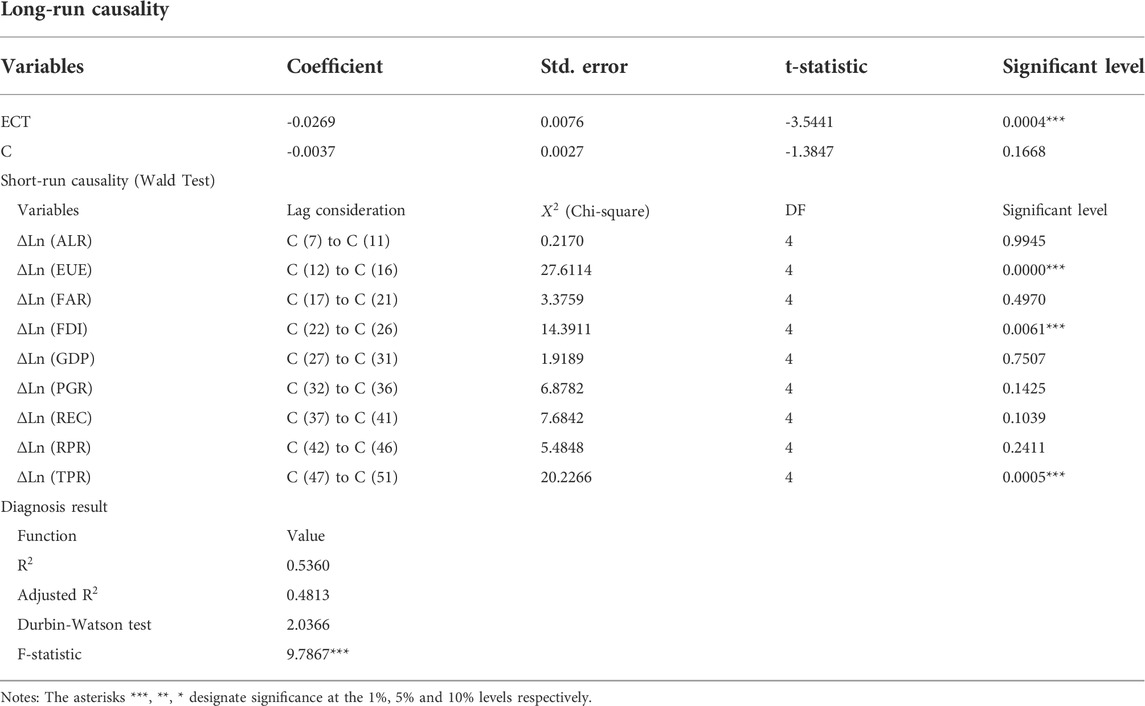
TABLE 7. VECM short-run and long-run interconnection.
Moreover, it is vital to diagnosis the validity of the VECM model. Generally, the reliability of the model depends on the normality of the residual, residual autocorrelation, heteroskedasticity, and stability tests. Accordingly, we apply Jarque-Bera statistic for normality test, Breusch-Godfrey Lagrange multiplier (LM) test (Breusch, 1978) for detecting autocorrelation, Breusch-Pagan-Godfrey test (also called LM test) (Godfrey, 1978; Breusch & Pagan, 1979) for heteroskedasticity test, and roots of the characteristic polynomial for stability diagnosis. VECM model of our study passes all the residual diagnosis tests, suggesting validity of our model and hence, can be used for analysis5. Additionally, Durbin-Watson test indicates robustness of absence of autocorrelation problem in the model6.
Pairwise Granger causality findings are presented in Table 8. The Granger causality analysis supports in viewing the true path of causation among the studied variables (Gyamfi, 2022). We notice absence of Granger causality between CO2-ALR, EUE-ALR, FDI-ALR, GDP-ALR, RPR-ALR, TPR-ALR, FAR-CO2, GDP-CO2, RPR-CO2, FAR-EUE, PGR-EUE, RPR-EUE, FDI-FAR, RPR-FAR, TPR-FAR, PGR-GDP, REC-GDP, RPR-GDP, REC-PGR, RPR-PGR, TPR-PGR, RPR-REC, TPR-RPR variables as p values for both cases are adequately high to accept both null hypotheses. Alvarado et al. (2018); Dyrstad et al. (2019); Awodumi & Adewuyi (2020) also found no pairwise relationship between GDP to CO2 in 151 countries, 27 OECD countries, and 5 African countries respectively. However, unidirectional Granger causal relationships are observed between the ALR-REC, EUE-CO2, FDI-EUE, FAR-ALR, GDP-FAR, REC-FAR, GDP-FDI, REC-FDI, RPR-FDI, EUE-GDP, ALR-PGR, CO2-PGR, FAR-PGR, FDI-PGR, CO2-REC, REC-TPR variables. The unidirectional relationship between EUE to GDP; EUE to CO2, and CO2 to REC is associated with the previous studies (Mbarek et al., 2018; Bekun et al., 2019); (Bekun et al., 2019; Chen et al., 2019; Mahmood et al., 2019); and (Sulaiman et al., 2013; Bölük & Mert, 2014; Bilgili et al., 2016; Ito, 2017; Bélaïd & Youssef, 2017; Balsalobre-Lorente et al., 2018; Hanif, 2018) respectively. Furthermore, results manifest that there are bidirectional causation running from the variables CO2, TPR, REC, EUE, TPR, and GDP to FDI, CO2, EUE, TPR, FDI, and TPR respectively, suggesting that each pair has both an owning and an inverse side. Evidence from the joint Granger causality represents except FAR and RPR, remaining variables ALR, CO2, EUE, FDI, GDP, PGR, REC, and TPR have unidirectional joint causal relationship to the studied variables.
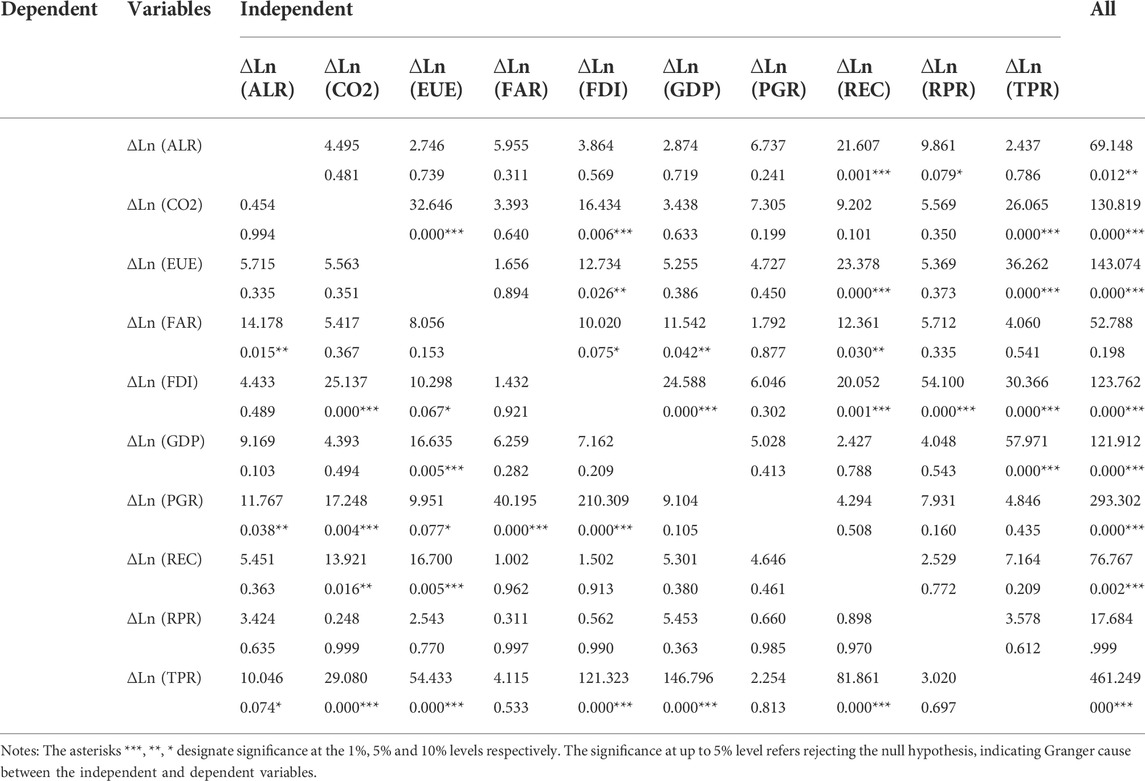
TABLE 8. Pairwise Granger causality test.
Figure 2 represents the Cholesky one standard deviation novelties impulse response functions (IRFs) adjusted by degree of freedom between the dependent variable CO2 emissions and independent variables ALR, EUE, FAR, FDI, GDP, PGR, REC, RPR, and TPR. The IRF is suitable for being able to elucidate the sign of the association and how long these upshots necessitate to take place. However, we exclude pairwise impulse response functions between independent variables due to the brevity. For demonstrating the findings, Figure 2A displays the response of ALR to CO2 that suggests ALR responds positively after the lag period 2 (1 lag = 1 year). The curve follows an upward trend till lag 15 and then it dies off. Figure 2B shows the positive response of EUE to CO2 from the beginning period although between the lag six and 7 it follows a downward trend, however after lag 9, it is flatter. Figure 2C exhibits negative response function of FAR to CO2 at most of the lag periods, but positive response is observed till 10th lag. The response function of FDI to CO2 emissions is represented in Figure 2D where we notice the curve follows upward-downward movement between the lag one to lag 15, after that it slowly follows the straight-line movement. Figure 2E unveils a positive and significant response function running from GDP to CO2 throughout the study periods. Figure 2F presents the response function of PGR to CO2 where positive upward-downward trends is detected till lag 16 and then it gets moved out almost in the same direction.
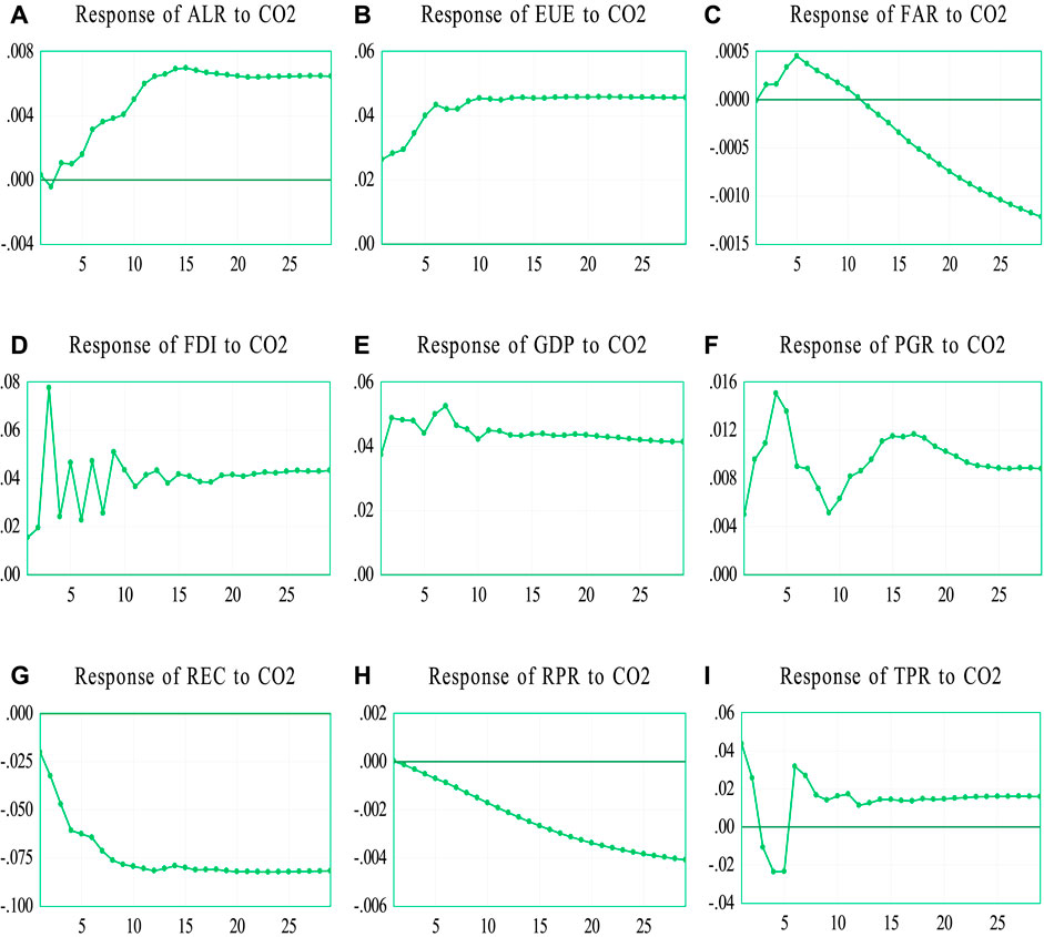
FIGURE 2. Impulse response to Cholesky one standard deviation (DOF adjusted) novelties. Notes: The horizontal axis of each impulse response function represents the sequence or observation of times, namely 1990 = 1, 1991 = 2, 1992 = 3, and so on. The vertical axis of each impulse response function expresses the impulse response.
Figures 2G,H show the negative impulse response function of REC and RPR to CO2 emissions. REC responds negatively to CO2 from the rudimentary lag period, however, RPR responds negatively to CO2 from break-even level. Surprisingly, both REC and RPR die off after following a static movement. Figure 2I denotes the response function of TPR to CO2 that indicates positive flatter trend after lag 12, moreover, negative response function is experimented after lag two to lag 6.
Generalized method of moments (GMM) estimators and fixed-effect regression results are exhibited in Table 9. We apply two kinds of GMM techniques, namely, GMM at difference, and orthogonal deviation GMM, along with fixed-effect OLS regression model to explore the significant relationship between the dependent and independent variables. We select fixed-effect OLS model among the pooled, fixed and random models according to F-test and Hausman test statistics. For depicting the results, we notice in model 1,2, and three that FDI, PGR, TPR have positive insignificant association with CO2 emissions, implying there are not much influences of FDI, PGR, TPR to the environmental condition in the oil-producing countries. These results infer that investment from outsiders, population growth, and trade integration not be seen as a chance to deploy as tools to reduce CO2 emissions in oil-producing countries. Feridun et al. (2006) also found insignificant positive linkage of trade integration with the CO2 emissions. However, it is observed that EUE and GDP affect the CO2 emissions positively and significantly in the both models, suggesting that more the energy use and gross domestic product (GDP), more the carbon dioxide emits. In oil-producing countries, using energy and higher GDP volume degrade the environmental pollution by increasing CO2 in the atmosphere, indicating that as income rises, preferences for manufactured goods are increased, as a result, producers must use more energy to keep up with the shift in demand, which results in the emission of CO2. This finding is associated with the studies of (Acaravci & Ozturk, 2010; Hanif, 2018a; Hanif et al., 2019) who found significant positive alliance between energy use and CO2 emissions in East Asia and the Pacific countries, Europe continent, and 25 developing Asian countries respectively. In EU region, countries are reluctant to control the adverse effect of CO2 emissions due to the higher dependent on the income level by emphasizing on economic development, energy use, bilateral trade, however, use of renewable energy is playing role as a safeguard against the brutal effect of increasing the CO2 emissions (Radmehr et al., 2021). Philip et al. (2022) documented that renewable energy mitigates the CO2 emissions Malaysia. Furthermore, a negative insignificant relationship is detected between REC and CO2 emissions in all the models, while the same linkage is found between RPR and CO2 emissions in model one and 2. It is surprising to see that energy use has a positive influence on CO2 emissions, while using renewable energy has a negative impact, indicating that switching to renewable energy from non-renewable energy could develop the environmental condition in oil-producing countries.
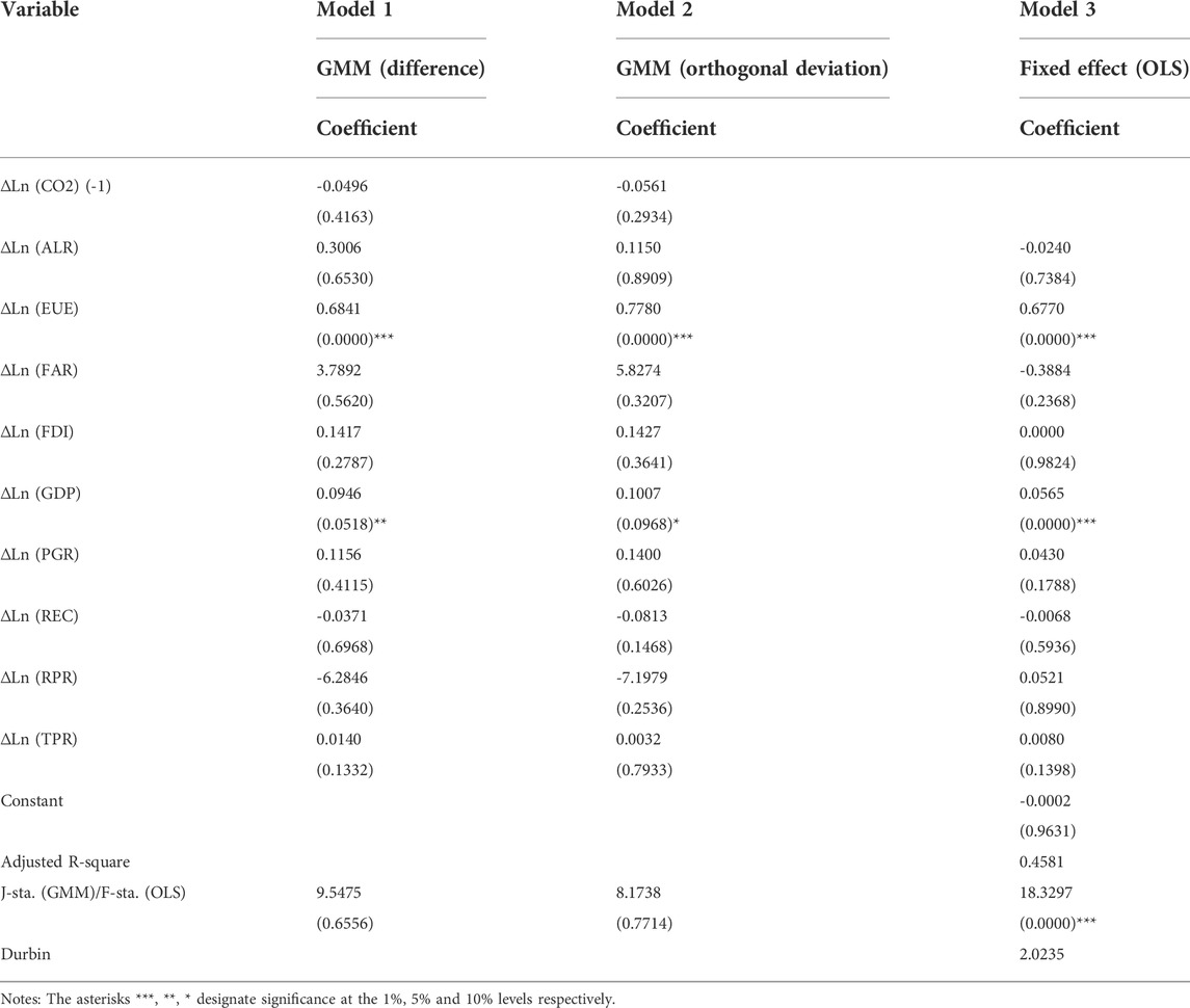
TABLE 9. GMM and fixed-effect estimations.
In diagnosis test results, adjusted R-square and Durbin-Watson test values indicate that the fixed-effect model is perfectly fit and there is absence of autocorrelation problem7. Furthermore, J-statistic values both coefficient and probability suggest appropriate GMM, model estimation.
The biggest threat of the current world is climate changes. The health of the world, mankind, species, and ecosystems are in grave jeopardy as a result of these atmospheric changes. In these instances, controlling the carbon dioxide (CO2) emissions is the main challenge to ensure a sustainable world environment. A plenty of macroeconomic factors both geographical and non-geographical are regularly contaminating the environmental conditions. Studies show that the amount of carbon emissions rises as the global economic growth accelerates. In the present literature, the sensitivity of CO2 emissions to changes in macroeconomic factors is well documented, but the effect of different factors on CO2 emissions in oil-producing countries is still undisclosed. So, this study’s principal goal is to look into the impact of population growth rate, forest area ratio, foreign direct investment, gross domestic product, trade percentage rate, energy use, renewable energy consumption, agricultural land ratio, and rural population rate on CO2 emissions in oil-producing nations in the world. The sample period of the datasets commences from 1990 to 2018, and based on the availability, the yearly datasets restrict the sample period, starting date, and ending date.
This paper applies several methods that provide perceptive evidence accordingly throughout the study. The Pedroni and Kao cointegration analysis tools demonstrate the presence of a long-run effect between the dependent variable- CO2 emissions and independent variable- ALR, EUE, FAR, FDI, GDP, PGR, REC, RPR, and TPR. To explore the short-run and long-run causation, the VECM approach unveils that long-run causality is running from the independent variables to the dependent variable. More particularly, EUE, FDI, TPR have both short- and long-run causal influence on the CO2 emissions, while only long-run Granger causality is moving from ALR, FAR, GDP, PGR, REC and RPR to CO2 emissions. The pairwise Granger causality evidences that CO2, TPR, REC, EUE, TPR, and GDP have bidirectional relationship with FDI, CO2, EUE, TPR, FDI, and TPR respectively, however, most of the pair experiences unidirectional and absence of causal linkages. Furthermore, the impulse response functions (IRFs) robust the findings of VECM long-run and short-run casual relationships.
The results of OLS based regressions indicate that EUE and GDP positively and significantly affect the CO2 emissions in oil-producing countries, suggesting high energy use and more gross domestic products deteriorate the environment by increasing CO2 emissions. However, other independent variables, namely, ALR, FAR, FDI, PGR, REC, RPR, and TPR have insignificant association with the CO2 emissions.
As the long-run consequences are found between climate change, economic growth, energy use, agriculture and rural development and CO2 emissions in oil-producing countries, the authority of the government and general public should be conscious about the above-mentioned factors to ensure the sustainable environment. Specifically, energy use should be minimized as much as possible or alternated by some other renewable energy sources that are environmentally friendly. Furthermore, emphasizing on controlling the population growth rate may help to enhance the favorable environmental condition over the short-run and long-run period. The producers should concentrate more on the long-run green products production rather than conventional products production in the short-run.
Moreover, our study has some limitations that guide future research. The more sophisticated methodology like, moments quantile regression and considering more oil-producing countries in the sample size with more variables may exhibit a better clear picture of CO2 emissions sensitivity.
The original contributions presented in the study are included in the article/supplementary material further inquiries can be directed to the corresponding authors.
Conceptualization, MN; data curation, MG and BD; formal analysis, MN and MG; funding acquisition, JS, MG, and BD; investigation, AH, BD, and JS; methodology, MG and MN; project administration, MG and JS; resources, MN, AH, and BD; software, MG, MN, and BD; supervision, MG, MN, and AH; validation, BD; writing —original draft, MN and MG; writing—review and editing, AH, JS, MN and MG.
This study was supported by the own fund of the authors.
The authors declare that the research was conducted in the absence of any commercial or financial relationships that could be construed as a potential conflict of interest.
All claims expressed in this article are solely those of the authors and do not necessarily represent those of their affiliated organizations, or those of the publisher, the editors and the reviewers. Any product that may be evaluated in this article, or claim that may be made by its manufacturer, is not guaranteed or endorsed by the publisher.
1BP Statistical Review of World Energy 2018 (67th edition). Available at: https://www.bp.com/content/dam/bp/business-sites/en/global/corporate/pdfs/energy-economics/statistical-review/bp-stats-review-2018-full-report.pdf (Accessed on 6 July 2022).
2An agency report entitled “Climate change: Nations must end oil production, report says”. Available at: https://punchng.com/climate-change-nations-must-end-oil-production-report-says/(Accessed on 6 July 2022).
3Available at: https://data.worldbank.org/indicator?tab=featured (Accessed on 23rd April 2022).
4Please see: Available at http://cruncheconometrix.blogspot.com/2018/03/time-series-analysis-lecture-4-part-1.html#:∼:text=If%20there%20is%20cointegration%3A,(in%20the%20long%20run (Accessed on third May 2022).
5Due to the brevity, explicit results are not demonstrated here. All test outcomes are available upon legitimate solicitation.
6Field (2009) denoted that the Durbin-Watson test value between one and three is not of the concern for autocorrelation.
7Field (2009) denoted that the Durbin-Watson test value between one and three is not of the concern for autocorrelation.
Abid, M. (2016). Impact of economic, financial, and institutional factors on CO2 emissions: Evidence from Sub-Saharan Africa economies. Util. Policy 41, 85–94. doi:10.1016/j.jup.2016.06.009
Acaravci, A., and Ozturk, I. (2010). On the relationship between energy consumption, CO2 emissions and economic growth in Europe. Energy 35 (12), 5412–5420. doi:10.1016/j.energy.2010.07.009
Adom, P. K., Amakye, K., Abrokwa, K. K., and Quaidoo, C. (2018). Estimate of transient and persistent energy efficiency in Africa: A stochastic frontier approach. Energy Convers. Manag. 166, 556–568. doi:10.1016/j.enconman.2018.04.038
Agboola, M. O., Bekun, F. V., and Joshua, U. (2021). Pathway to environmental sustainability: Nexus between economic growth, energy consumption, CO2 emission, oil rent and total natural resources rent in Saudi Arabia. Resour. Policy 74, 102380. doi:10.1016/j.resourpol.2021.102380
Al-mulali, U. (2012). Factors affecting CO2 emission in the Middle East: A panel data analysis. Energy 44 (1), 564–569. doi:10.1016/j.energy.2012.05.045
Alataş, S. (2022). Do environmental technologies help to reduce transport sector CO2 emissions? Evidence from the EU15 countries. Res. Transp. Econ. 91, 101047. doi:10.1016/j.retrec.2021.101047
Albulescu, C. T., Artene, A. E., Luminosu, C. T., and Tămășilă, M. (2020). CO2 emissions, renewable energy, and environmental regulations in the EU countries. Environ. Sci. Pollut. Res. 27 (27), 33615–33635. doi:10.1007/s11356-019-06155-1
Alkathery, M. A., and Chaudhuri, K. (2021). Co-movement between oil price, CO2 emission, renewable energy and energy equities: Evidence from GCC countries. J. Environ. Manag. 297, 113350. doi:10.1016/j.jenvman.2021.113350
Alvarado, R., Ponce, P., Criollo, A., Córdova, K., and Khan, M. K. (2018). Environmental degradation and real per capita output: New evidence at the global level grouping countries by income levels. J. Clean. Prod. 189, 13–20. doi:10.1016/j.jclepro.2018.04.064
Andersson, F. N. G., and Karpestam, P. (2013). CO2 emissions and economic activity: Short- and long-run economic determinants of scale, energy intensity and carbon intensity. Energy Policy 61, 1285–1294. doi:10.1016/j.enpol.2013.06.004
Anser, M. K., Yousaf, Z., Awan, U., Nassani, A. A., Qazi Abro, M. M., and Zaman, K. (2020). Identifying the carbon emissions damage to international tourism: Turn a blind eye. Sustainability 12 (5), 1937. doi:10.3390/su12051937
Antweiler, W., Copeland, B., and Taylor, M. S. (2001). Is free trade good for the environment? Am. Econ. Rev. 91, 877–908. doi:10.1257/aer.91.4.877
Awodumi, O. B., and Adewuyi, A. O. (2020). The role of non-renewable energy consumption in economic growth and carbon emission: Evidence from oil producing economies in Africa. Energy Strategy Rev. 27, 100434. doi:10.1016/j.esr.2019.100434
Azam, M., and Khan, A. Q. (2017). Growth-corruption-health triaca and environmental degradation: Empirical evidence from Indonesia, Malaysia, and Thailand. Environ. Sci. Pollut. Res. 24 (19), 16407–16417. doi:10.1007/s11356-017-9299-4
Bakucs, Z., and Fertő, I. (2011). Innovation and output in OECD countries: Implications upon emerging economies. Int. J. Innovation Learn. 9 (4), 388–400. doi:10.1504/IJIL.2011.040537
Balsalobre-Lorente, D., Shahbaz, M., Roubaud, D., and Farhani, S. (2018). How economic growth, renewable electricity and natural resources contribute to CO2 emissions? Energy Policy 113, 356–367. doi:10.1016/j.enpol.2017.10.050
Bekun, F. V., Alola, A. A., and Sarkodie, S. A. (2019). Toward a sustainable environment: Nexus between CO2 emissions, resource rent, renewable and nonrenewable energy in 16-EU countries. Sci. Total Environ. 657, 1023–1029. doi:10.1016/j.scitotenv.2018.12.104
Bélaïd, F., and Youssef, M. (2017). Environmental degradation, renewable and non-renewable electricity consumption, and economic growth: Assessing the evidence from Algeria. Energy Policy 102, 277–287. doi:10.1016/j.enpol.2016.12.012
Bilan, Y., Streimikiene, D., Vasylieva, T., Lyulyov, O., Pimonenko, T., and Pavlyk, A. (2019). Linking between renewable energy, CO2 emissions, and economic growth: Challenges for candidates and potential candidates for the EU membership. Sustain. Switz. 11 (6), 1528. doi:10.3390/su11061528
Bilgili, F., Koçak, E., and Bulut, Ü. (2016). The dynamic impact of renewable energy consumption on CO2 emissions: A revisited environmental kuznets curve approach. Renew. Sustain. Energy Rev. 54, 838–845. doi:10.1016/j.rser.2015.10.080
Blanco, L., Gonzalez, F., and Ruiz, I. (2013). The impact of FDI on CO2 emissions in Latin America. Oxf. Dev. Stud. 41 (1), 104–121. doi:10.1080/13600818.2012.732055
Bölük, G., and Mert, M. (2014). Fossil & renewable energy consumption, GHGs (greenhouse gases) and economic growth: Evidence from a panel of EU (European Union) countries. Energy 74, 439–446. doi:10.1016/j.energy.2014.07.008
Breitung, J., and Candelon, B. (2005). Purchasing power parity during currency crises: A panel unit root test under structural breaks. Rev. World Econ. 141 (1), 124–140. doi:10.1007/s10290-005-0018-8
Breusch, T. S., and Pagan, A. R. (1979). A simple test for heteroscedasticity and random coefficient variation. Econometrica 47 (5), 1287–1294. doi:10.2307/1911963
Breusch, T. S. (1978). Testing for autocorrelation in dynamic linear models. Aust. Econ. Pap. 17 (31), 334–355. doi:10.1111/j.1467-8454.1978.tb00635.x
Castán Broto, V. (2017). Urban governance and the politics of climate change. World Dev. 93, 1–15. doi:10.1016/j.worlddev.2016.12.031
Chen, Y., Wang, Z., and Zhong, Z. (2019). CO2 emissions, economic growth, renewable and non-renewable energy production and foreign trade in China. Renew. Energy 131, 208–216. doi:10.1016/j.renene.2018.07.047
Chevallier, J., Khuong Nguyen, D., and Carlos Reboredo, J. (2019). A conditional dependence approach to CO2-energy price relationships. Energy Econ. 81, 812–821. doi:10.1016/j.eneco.2019.05.010
Cole, M. A., and Elliott, R. J. R. (2003). Determining the trade–environment composition effect: The role of capital, labor and environmental regulations. J. Environ. Econ. Manag. 46 (3), 363–383. doi:10.1016/S0095-0696(03)00021-4
Danish, , Wang, B., and Wang, Z. (2018). Imported technology and CO2 emission in China: Collecting evidence through bound testing and VECM approach. Renew. Sustain. Energy Rev. 82, 4204–4214. doi:10.1016/j.rser.2017.11.002
Dyrstad, J. M., Skonhoft, A., Christensen, M. Q., and Ødegaard, E. T. (2019). Does economic growth eat up environmental improvements? Electricity production and fossil fuel emission in OECD countries 1980–2014. Energy Policy 125, 103–109. doi:10.1016/j.enpol.2018.10.051
Ebohon, O. J., and Ikeme, A. J. (2006). Decomposition analysis of CO2 emission intensity between oil-producing and non-oil-producing sub-Saharan African countries. Energy Policy 34 (18), 3599–3611. doi:10.1016/j.enpol.2004.10.012
Feridun, M., Ayadi, F. S., and Balouga, J. (2006). Impact of trade liberalization on the environment in developing countries: The case of Nigeria. J. Dev. Soc. 22 (1), 39–56. doi:10.1177/0169796X06062965
Field, Andy (2009). Discovering statistics using SPSS. 3rd ed. Thousand Oaks, CA: SAGE Publications Ltd.
Gavenas, E., Rosendahl, K. E., and Skjerpen, T. (2015). CO2-emissions from Norwegian oil and gas extraction. Energy 90, 1956–1966. doi:10.1016/j.energy.2015.07.025
Godfrey, L. G. (1978). Testing against general autoregressive and moving average error models when the regressors include lagged dependent variables. Econometrica 46 (6), 1293–1301. doi:10.2307/1913829
Granger, C. W. J. (1969). Investigating causal relations by econometric models and cross-spectral methods. Econometrica 37 (3), 424–438. doi:10.2307/1912791
Gyamfi, B. A. (2022). Consumption-based carbon emission and foreign direct investment in oil-producing sub-sahara african countries: The role of natural resources and urbanization. Environ. Sci. Pollut. Res. 29 (9), 13154–13166. doi:10.1007/s11356-021-16509-3
Hanif, I., Aziz, B., and Chaudhry, I. S. (2019). Carbon emissions across the spectrum of renewable and nonrenewable energy use in developing economies of Asia. Renew. Energy 143, 586–595. doi:10.1016/j.renene.2019.05.032
Hanif, I. (2018). Impact of economic growth, nonrenewable and renewable energy consumption, and urbanization on carbon emissions in Sub-Saharan Africa. Environ. Sci. Pollut. Res. 25 (15), 15057–15067. doi:10.1007/s11356-018-1753-4
Hanif, I. (2018a). Impact of fossil fuels energy consumption, energy policies, and urban sprawl on carbon emissions in East Asia and the pacific: A panel investigation. Energy Strategy Rev. 21, 16–24. doi:10.1016/j.esr.2018.04.006
Hansen, L. P. (1982). Large sample properties of generalized method of moments estimators. Econometrica 50 (4), 1029–1054. doi:10.2307/1912775
Hao, Y., Li, Z., Su, Y., Kong, C., Chen, H., and Meng, Y. (2022). Experimental investigation of CO2 storage and oil production of different CO2 injection methods at pore-scale and core-scale. Energy 254, 124349. doi:10.1016/j.energy.2022.124349
Hasanov, F. J., Liddle, B., and Mikayilov, J. I. (2018). The impact of international trade on CO2 emissions in oil exporting countries: Territory vs consumption emissions accounting. Energy Econ. 74, 343–350. doi:10.1016/j.eneco.2018.06.004
Hassan, S. T., Danish, , Khan, S. U.-D., Xia, E., and Fatima, H. (2020). Role of institutions in correcting environmental pollution: An empirical investigation. Sustain. Cities Soc. 53, 101901. doi:10.1016/j.scs.2019.101901
Hassan, S. T., Danish, Salah-Ud-Din, Awais Baloch, M., and Tarar, Z. H. (2020a). Is nuclear energy a better alternative for mitigating CO2 emissions in BRICS countries? An empirical analysis. Nucl. Eng. Technol. 52 (12), 2969–2974. doi:10.1016/j.net.2020.05.016
He, K., Huo, H., Zhang, Q., He, D., An, F., Wang, M., et al. (2005). Oil consumption and CO2 emissions in China’s road transport: Current status, future trends, and policy implications. Energy Policy 33 (12), 1499–1507. doi:10.1016/j.enpol.2004.01.007
Ibitoye, F. I., and Akinbami, J.-F. K. (1999). Strategies for implementation of CO2-mitigation options in Nigeria’s energy sector. Appl. Energy 63 (1), 1–16. doi:10.1016/S0306-2619(99)00015-X
IEA (2013). Sustainable Energy for All (SE4ALL)- Global Tracking Framework Report, 60. Paris, France: World Development, 84–98.
IEA (2022). Global energy review: CO2 emissions in 2021. Paris: IEA. https://www.iea.org/reports/global-energy-review-co2-emissions-in-2021-2.
Ike, G. N., Usman, O., and Sarkodie, S. A. (2020). Testing the role of oil production in the environmental Kuznets curve of oil producing countries: New insights from Method of Moments Quantile Regression. Sci. Total Environ. 711, 135208. doi:10.1016/j.scitotenv.2019.135208
İnal, V., Addi, H. M., Çakmak, E. E., Torusdağ, M., and Çalışkan, M. (2022). The nexus between renewable energy, CO2 emissions, and economic growth: Empirical evidence from African oil-producing countries. Energy Rep. 8, 1634–1643. doi:10.1016/j.egyr.2021.12.051
IPCC (2007). The physical science basis. Contribution of working group I to the fourth assessment report of the Intergovernmental Panel on Climate Change. Cambridge, United Kingdom: Cambridge University Press, 113–119.
Islam, M. M., Khan, M. K., Tareque, M., Jehan, N., and Dagar, V. (2021). Impact of globalization, foreign direct investment, and energy consumption on CO2 emissions in Bangladesh: Does institutional quality matter? Environ. Sci. Pollut. Res. 28 (35), 48851–48871. doi:10.1007/s11356-021-13441-4
Ito, K. (2017). CO2 emissions, renewable and non-renewable energy consumption, and economic growth: Evidence from panel data for developing countries. Int. Econ. 151, 1–6. doi:10.1016/j.inteco.2017.02.001
Kao, C. (1999). Spurious regression and residual-based tests for cointegration in panel data. J. Econ. 90 (1), 1–44. doi:10.1016/S0304-4076(98)00023-2
Kasman, A., and Duman, Y. S. (2015). CO2 emissions, economic growth, energy consumption, trade and urbanization in new EU member and candidate countries: A panel data analysis. Econ. Model. 44, 97–103. doi:10.1016/j.econmod.2014.10.022
Kassouri, Y., Bilgili, F., and Kuşkaya, S. (2022). A wavelet-based model of world oil shocks interaction with CO2 emissions in the US. Environ. Sci. Policy 127, 280–292. doi:10.1016/j.envsci.2021.10.020
Khan, A. Q., Saleem, N., and Fatima, S. T. (2018). Financial development, income inequality, and CO2 emissions in Asian countries using STIRPAT model. Environ. Sci. Pollut. Res. 25 (7), 6308–6319. doi:10.1007/s11356-017-0719-2
Khan, M. K., Teng, J. Z., Khan, M. I., and Khan, M. O. (2019). Impact of globalization, economic factors and energy consumption on CO2 emissions in Pakistan. Sci. Total Environ. 688, 424–436. doi:10.1016/j.scitotenv.2019.06.065
King, Maxwell L., and Goh, Kim-Leng (2002). Improvements to the Wald test". Handbook of applied econometrics and statistical inference. 1 edition. New York: Marcel Dekker, 251–276. 0-8247-0652-8.
Krantz, G., Brandao, M., Hedenqvist, M., and Nilsson, F. (2022). Indirect CO2 emissions caused by the fuel demand switch in international shipping. Transp. Res. Part D Transp. Environ. 102, 103164. doi:10.1016/j.trd.2021.103164
Le, T. H., Chang, Y., and Park, D. (2016). Trade openness and environmental quality: International evidence. Energy Policy 92, 45–55. doi:10.1016/j.enpol.2016.01.030
Levin, A., Lin, C.-F., and James Chu, C.-S. (2002). Unit root tests in panel data: Asymptotic and finite-sample properties. J. Econ. 108 (1), 1–24. doi:10.1016/S0304-4076(01)00098-7
Li, B., and Haneklaus, N. (2022). Reducing CO2 emissions in G7 countries: The role of clean energy consumption, trade openness and urbanization. Energy Rep. 8, 704–713. doi:10.1016/j.egyr.2022.01.238
Liew, V. K. (2004). Which lag length selection criteria should we employ? Econ. Bull. AccessEcon 3 (33), 1–9.
Lindstad, E., Eskeland, G. S., Rialland, A., and Valland, A. (2020). Decarbonizing maritime transport: The importance of engine technology and regulations for LNG to serve as a transition fuel. Sustainability 12 (21), 8793. doi:10.3390/su12218793
Lindstad, H. E., and Eskeland, G. S. (2016). Environmental regulations in shipping: Policies leaning towards globalization of scrubbers deserve scrutiny. Transp. Res. Part D Transp. Environ. 47, 67–76. doi:10.1016/j.trd.2016.05.004
Lindstad, H., Eskeland, G. S., Psaraftis, H., Sandaas, I., and Strømman, A. H. (2015). Maritime shipping and emissions: A three-layered, damage-based approach. Ocean. Eng. 110, 94–101. doi:10.1016/j.oceaneng.2015.09.029
Luqman, M., Ahmad, N., and Bakhsh, K. (2019). Nuclear energy, renewable energy and economic growth in Pakistan: Evidence from non-linear autoregressive distributed lag model. Renew. Energy 139, 1299–1309. doi:10.1016/j.renene.2019.03.008
Mahdi Ziaei, S. (2015). Effects of financial development indicators on energy consumption and CO2 emission of European, East Asian and Oceania countries. Renew. Sustain. Energy Rev. 42, 752–759. doi:10.1016/j.rser.2014.10.085
Mahmood, N., Wang, Z., and Hassan, S. T. (2019). Renewable energy, economic growth, human capital, and CO2 emission: An empirical analysis. Environ. Sci. Pollut. Res. 26 (20), 20619–20630. doi:10.1007/s11356-019-05387-5
Malla, S. (2009). CO2 emissions from electricity generation in seven asia-pacific and north American countries: A decomposition analysis. Energy Policy 37 (1), 1–9. doi:10.1016/j.enpol.2008.08.010
Martínez-Zarzoso, I., Bengochea-Morancho, A., and Morales-Lage, R. (2007). The impact of population on CO2 emissions: Evidence from European countries. Environ. Resour. Econ. (Dordr). 38 (4), 497–512. doi:10.1007/s10640-007-9096-5
Mbarek, M., Saidi, K., and Rahman, M. M. (2018). Renewable and non-renewable energy consumption, environmental degradation and economic growth in Tunisia. Qual. Quant. 52 (3), 1105–1119. doi:10.1007/s11135-017-0506-7
Neal, T. (2014). Panel cointegration analysis with xtpedroni. Stata J. 14 (3), 684–692. doi:10.1177/1536867X1401400312
Oh, I., Wehrmeyer, W., and Mulugetta, Y. (2010). Decomposition analysis and mitigation strategies of CO2 emissions from energy consumption in South Korea. Energy Policy 38 (1), 364–377. doi:10.1016/j.enpol.2009.09.027
Omay, T., and Öznur Kan, E. (2010). Re-examining the threshold effects in the inflation–growth nexus with cross-sectionally dependent non-linear panel: Evidence from six industrialized economies. Econ. Model. 27 (5), 996–1005. doi:10.1016/j.econmod.2010.04.011
Pachiyappan, D., Ansari, Y., Alam, M. S., Thoudam, P., Alagirisamy, K., and Manigandan, P. (2021). Short and long-run causal effects of CO2 emissions, energy use, gdp and population growth: Evidence from India using the ardl and vecm approaches. Energies 14 (24), 8333. doi:10.3390/en14248333
Pan, S., Tachega, M., Amowine, N., and Ackaah, W. (2018). The relationship between foreign aid and growth: A comparative analysis of low income, lower-middle income and upper-middle-income african countries. J. Econ. Sustain. Dev. 9 (6), 66–80.
Paraschiv, S., and Paraschiv, L. S. (2020). Trends of carbon dioxide (CO2) emissions from fossil fuels combustion (coal, gas and oil) in the EU member states from 1960 to 2018. Energy Rep. 6, 237–242. doi:10.1016/j.egyr.2020.11.116
Pedroni, P. (1999). Critical values for cointegration tests in heterogeneous panels with multiple regressors. Oxf. Bull. Econ. Stat. 61 (S1), 653–670. doi:10.1111/1468-0084.0610s1653
Philip, L. D., Emir, F., and Udemba, E. N. (2022). Investigating possibility of achieving sustainable development goals through renewable energy, technological innovation, and entrepreneur: A study of global best practice policies. Environ. Sci. Pollut. Res. 29, 60302–60313. doi:10.1007/s11356-022-20099-z
Radmehr, R., Henneberry, S. R., and Shayanmehr, S. (2021). Renewable energy consumption, CO2 emissions, and economic growth nexus: A simultaneity spatial modeling analysis of EU countries. Struct. Change Econ. Dyn. 57, 13–27. doi:10.1016/j.strueco.2021.01.006
Rogelj, J., McCollum, D. L., Reisinger, A., Meinshausen, M., and Riahi, K. (2013). Probabilistic cost estimates for climate change mitigation. Nature 493 (7430), 79–83. doi:10.1038/nature11787
Saidi, K., and Omri, A. (2020). Reducing CO2 emissions in OECD countries: Do renewable and nuclear energy matter? Prog. Nucl. Energy 126, 103425. doi:10.1016/j.pnucene.2020.103425
Salahuddin, M., Alam, K., and Ozturk, I. (2016). The effects of internet usage and economic growth on CO2 emissions in OECD countries: A panel investigation. Renew. Sustain. Energy Rev. 62, 1226–1235. doi:10.1016/j.rser.2016.04.018
Salari, M., Javid, R. J., and Noghanibehambari, H. (2021). The nexus between CO2 emissions, energy consumption, and economic growth in the U.S. Econ. Anal. Policy 69, 182–194. doi:10.1016/j.eap.2020.12.007
Sarpong, S. Y., and Bein, M. A. (2020). The relationship between good governance and CO2 emissions in oil- and non-oil-producing countries: A dynamic panel study of sub-saharan Africa. Environ. Sci. Pollut. Res. 27 (17), 21986–22003. doi:10.1007/s11356-020-08680-w
Sheinbaum, C., Ruíz, B. J., and Ozawa, L. (2011). Energy consumption and related CO2 emissions in five Latin American countries: Changes from 1990 to 2006 and perspectives. Energy 36 (6), 3629–3638. doi:10.1016/j.energy.2010.07.023
Sikder, M., Wang, C., Yao, X., Huai, X., Wu, L., KwameYeboah, F., et al. (2022). The integrated impact of GDP growth, industrialization, energy use, and urbanization on CO2 emissions in developing countries: Evidence from the panel ARDL approach. Sci. Total Environ. 837, 155795. doi:10.1016/j.scitotenv.2022.155795
Sinha, A., and Shahbaz, M. (2018). Estimation of environmental kuznets curve for CO2 emission: Role of renewable energy generation in India. Renew. Energy 119, 703–711. doi:10.1016/j.renene.2017.12.058
Sulaiman, J., Azman, A., and Saboori, B. (2013). The potentialof renewable energy: Using the environmental kuznets curve model. Am. J. Environ. Sci. 9 (2), 103–112. doi:10.3844/ajessp.2013.103.112
Tiwari, C., and Mishra, M. (2016). Testing the CO2 emissions convergence: Evidence from asian countries. IIM Kozhikode Soc. Manag. Rev. 6 (1), 67–72. doi:10.1177/2277975216674073
Udemba, E. N., and Tosun, M. (2022). Energy transition and diversification: A pathway to achieve sustainable development goals (SDGs) in Brazil. Energy 239, 122199. doi:10.1016/j.energy.2021.122199
Udemba, E. N., Emir, F., and Philip, L. D. (2022). Mitigating poor environmental quality with technology, renewable and entrepreneur policies: A symmetric and asymmetric approaches. Renew. Energy 189, 997–1006. doi:10.1016/j.renene.2022.03.060
Ullah, S., Ozturk, I., Usman, A., Majeed, M. T., and Akhtar, P. (2020). On the asymmetric effects of premature deindustrialization on CO2 emissions: Evidence from Pakistan. Environ. Sci. Pollut. Res. 27 (12), 13692–13702. doi:10.1007/s11356-020-07931-0
UNCTAD (2018). Global foreign direct investment flows fell sharply in 2017. Retrieved from: https://unctad.org/news/global-foreign-direct-investment-flows-fell-sharply-2017.
Wang, K. H., Su, C. W., Lobonţ, O. R., and Umar, M. (2021). Whether crude oil dependence and CO2 emissions influence military expenditure in net oil importing countries? Energy Policy 153, 112281. doi:10.1016/j.enpol.2021.112281
Wolfowitz, J. (1952). Abraham Wald, 1902-1950. Ann. Math. Stat. 23 (1), 1–13. doi:10.1214/aoms/1177729480
Wooldridge, J. M. (2009). On estimating firm-level production functions using proxy variables to control for unobservables. Econ. Lett. 104 (3), 112–114. doi:10.1016/j.econlet.2009.04.026
Yee, T. W. (2021). On the hauck–donner effect in Wald tests: Detection, tipping points, and parameter space characterization. J. Am. Stat. Assoc., 1–12. doi:10.1080/01621459.2021.1886936
Yusuf, A. M., Abubakar, A. B., and Mamman, S. O. (2020). Relationship between greenhouse gas emission, energy consumption, and economic growth: Evidence from some selected oil-producing african countries. Environ. Sci. Pollut. Res. 27 (13), 15815–15823. doi:10.1007/s11356-020-08065-z
Keywords: CO2 emissions, oil-producing countries, climate change, economic growth, energy use, Pedroni cointegration, VECM, GMM model
Citation: Gazi MAI, Nahiduzzaman M, Shaturaev J, Dhar BK and Halim MA (2022) Dynamic Nexus between macroeconomic factors and CO2 emissions: Evidence from oil-producing countries. Front. Environ. Sci. 10:1005814. doi: 10.3389/fenvs.2022.1005814
Received: 28 July 2022; Accepted: 28 September 2022;
Published: 28 October 2022.
Edited by:
Faik Bilgili, Erciyes University, TurkeyReviewed by:
Edmund Udemba, Gelişim Üniversitesi, TurkeyCopyright © 2022 Gazi, Nahiduzzaman, Shaturaev, Dhar and Halim. This is an open-access article distributed under the terms of the Creative Commons Attribution License (CC BY). The use, distribution or reproduction in other forums is permitted, provided the original author(s) and the copyright owner(s) are credited and that the original publication in this journal is cited, in accordance with accepted academic practice. No use, distribution or reproduction is permitted which does not comply with these terms.
*Correspondence: Md. Nahiduzzaman, aW5mby5uYWhpZHV6emFtYW4uYmRAZ21haWwuY29t; Bablu Kumar Dhar, YmFibHUua3VtQG1haGlkb2wuYWMudGg=
Disclaimer: All claims expressed in this article are solely those of the authors and do not necessarily represent those of their affiliated organizations, or those of the publisher, the editors and the reviewers. Any product that may be evaluated in this article or claim that may be made by its manufacturer is not guaranteed or endorsed by the publisher.
Research integrity at Frontiers
Learn more about the work of our research integrity team to safeguard the quality of each article we publish.