Landscape patterns and their spatial associations with ecosystem service balance: Insights from a rapidly urbanizing coastal region of southeastern China

Abstract: Assessing ecosystem service (ES) balance and exploring critical drivers are crucial for landscape management. However, a lack of understanding of the determinants of the ecosystem service supply–demand budget, their spillover effects, and spatial variabilities offsets the efficacy of landscape planning and ecosystem conservation. This novel study attempted to close this gap by quantifying ecosystem service budget using an expert knowledge-based supply–demand matrix and explored its dependencies through spatial econometrics and geographically weighted regression approaches instead of using ordinary model simulation and conventional statistical analysis. The overall patterns of ecosystem service balance in the southeastern coast were found to have remained stable in 1980, 2000, and 2017, although remarkable ecosystem service deficits were identified in hotspots of rapid urbanization. The ecosystem service balance was negatively associated with the proportions of built-up land and cropland (p < 0.0001) and exhibited positive associations with the proportions of woodland and grassland (p < 0.0001). Landscape structure and population density were identified as the primary determinants of ecosystem service balance and exhibited spatial variability and spillover effects (i.e., determining ecosystem service balance in both individual and adjacent units). These findings demonstrate the significance of spatial disparities and external effects of determinants of the supply–demand budget in integrative landscape governance. Consequently, localized and targeted strategies for landscape planning are increasingly needed to optimize landscape configuration and alleviate ecosystem service imbalance according to individual socioeconomic conditions and landscape structures. In addition, the spillover effects demonstrate that the maintenance of regional ecosystem service balance and ecosystem sustainability depends not only on individual areas but also on cross-regional collaborations with neighboring regions. These findings have critical implications on strategy formulation for coastal landscape management and ecosystem sustainability.

1 Introduction

Ecosystem services (ESs) link social systems and natural ecosystems and play extremely important roles in sustaining human survival and well-being and achieving sustainable development goals through optimized environmental management (Costanza et al., 2017; Mandle et al., 2020). An integrated ES assessment involves the supply and demand of ESs, which reflect the supply capacity of natural ecosystems and the actual demands required or desired by human society, respectively (Burkhard et al., 2012, 2014). Existing studies have mostly focused on quantifying and mapping the supply potential of natural ecosystems through multiple indicators, frameworks, biophysical models, and economic valuation approaches (e.g., Chaplin-Kramer et al., 2019; Ouyang et al., 2020; Zhang et al., 2021) and identifying the climatic, topographical, vegetation, socioeconomic, and landscape variables that determine the ES supply capacity (e.g., Turpie et al., 2017; Wilkerson et al., 2018). However, in comparison with the supply side, ES demand has not received sufficient attention, and the quantification framework is not well established (Costanza et al., 2017; Tao et al., 2018; Mandle et al., 2020).

An integrated ES assessment that incorporates the demand aspect into assessment can effectively identify the mismatch between supply and demand, support policy formulation and decisions regarding ES management, and balance the spatial and temporal disparities in the supply–demand budget (Castillo-Eguskitza et al., 2018; Chaplin-Kramer et al., 2019). In the past decade, a series of studies have attempted to integrate the demand aspect into ES assessment by quantifying and comparing specific indicators, including carbon sequestration, soil erosion control, hydrological regulation, food provision, and cultural services, in a particular ecosystem category (e.g., Campagne et al., 2018; Ma et al., 2019; Liu et al., 2020). Multiple approaches, including expert knowledge (Sun et al., 2020; Jiang et al., 2021a), questionnaire surveys (Castillo-Eguskitza et al., 2018), monetary value (Liu et al., 2021; Wang et al., 2021), and model simulation (Larondelle and Lauf, 2016; Yu et al., 2021; Zhang et al., 2021), have been adopted to quantify both sides of ESs. In particular, the level of demand for ESs by communities and residents in Spain was quantified through a questionnaire survey (Castillo-Eguskitza et al., 2018). Peng et al. (2020) investigated the spatial disparities in supply–demand balance based on the land use and land cover (LULC) category and expert knowledge in rapidly expanding city clusters in southern China. Chaplin-Kramer et al. (2019) projected the future supply and demand of ESs on a global scale based on model simulation and scenario analysis. The applicability of these methods varies in different cases according to data requirements and parameter settings. The model simulation approach largely relies on input parameters and spatially explicit data; thus, it is normally limited by data accessibility (Blanco et al., 2017). Although theoretically feasible for community- and county-scale studies, a questionnaire survey is not practically suitable for regional or continental assessments (Burkhard et al., 2014). The monetary value approach normally reflects the total value of ESs without a good spatially explicit representation that can reveal the spatial mismatches of supply and demand sides (Liu et al., 2021; Wang et al., 2021).

Additionally, ES supply generally reflects the beneficial function supplied by natural ecosystems through a combination of biophysical indicators, whereas ES demand is normally indicated by preferences, perceptions, market values, and actual consumption; thus, different measurement units constrain the direct comparison of both sides (Burkhard et al., 2014; Peng et al., 2020). The empirical knowledge method assumes that landscape patterns (i.e., LULC categories) determine ecological functions and ESs and then alter the supply–demand relationship. A proposed supply–demand matrix model takes the LULC category as a proxy and utilizes (semi-)empirical expert knowledge to quantify the supply–demand balance (Burkhard et al., 2014). Although this approach does not establish complete quantification methodologies, it can quickly obtain relatively reliable results without relying on complex models and input parameters, particularly for the assessment of cultural services (Sun et al., 2020).

For the optimization of landscape configuration and maintenance and enhancement of ecosystem sustainability, revealing the driving factors and influencing mechanisms of the ES supply–demand budget is as crucial as that of ES budget quantification (Sun et al., 2020; Jiang et al., 2021a). The formation, delivery, and circulation of matter and energy within a certain space (e.g., coenobium, ecosystem, watershed, and administrative unit) exhibit spillover effects on neighboring regions because the landscape compositions and biophysical/biogeochemical processes are interconnected (Li et al., 2019a; Li et al., 2019b; Zhang et al., 2022). Thereby, spatial attributes and spillover effects are supposed to be sufficiently revealed and integrated into landscape conservation and environmental governance (Wang et al., 2021; Zhang et al., 2021). However, previous literature lack sufficient understanding of geographic variations in the determinants of ES budgets and their spatial dependences and spillover effects (Chi and Ho, 2018). These findings have largely focused on individual units or local scales and neglected the spatial variability of important determinative factors from a regional perspective (Wang et al., 2021; Zhang et al., 2021). Moreover, the spillover effects of determinants have not been examined by commonly adopted statistical approaches, such as the least squares approach (Li et al., 2019a; Li et al., 2019b), random forest model (Liu et al., 2021), structural equation simulation (Jiang et al., 2021b), linear regression analysis (Wang et al., 2021), and other conventional econometric models (LeSage et al., 2009), because the spatial information is not taken into account in these models (Chi and Ho, 2018). Consequently, the external effects of determinants on strategy formulation in terms of landscape management have rarely been revealed (Jiang et al., 2021a; Zhang et al., 2022).

The southeastern coastal area of China has been characterized by rapid economic development, urban sprawl, and population expansion over the past 4 decades, which has led to inappropriate agricultural reclamation, deforestation, and other development and construction practices (Jia et al., 2018). This region suffers from the degradation of ecological function and resource scarcity as well as a severe mismatch and imbalance between the supply and demand of ESs (Zhang et al., 2021). We selected coastal areas as a case study to reveal the spatiotemporal evolution of the ES budget and identify the determinants and their spillover effects. Considering the limitations and knowledge gaps in existing literature, the main objectives of the current study were 1) to identify the spatial disparities of ES budgets for three important time nodes (1980, 2000, and 2018) based on the supply–demand matrix proposed according to expert knowledge, and discuss their responses to human disturbance and policy intervention-induced changes in landscape compositions; 2) to determine the critical dependences of the ES budget and their spatial disparities and spillover effects using spatial econometrics and geographically weighted regression (GWR) approaches; 3) to probe the implications of spatial dependencies of ES balance on the optimization of landscape configuration. The novelty of this study is in revealing the spatial associations of determinants of ES balance, in particular, in terms of their spillover effect and spatial variability, which distinguishes this study from previous studies that use ordinary model simulation and conventional statistical analysis. The research findings are expected to reconcile the mismatch between supply and demand sides of ESs, further improve the efficacy of landscape management, thereby supporting ecosystem conservation and contributing to coastal sustainable development.

2 Materials and methods

2.1 Study site

The study site (Figure 1A) is situated in the southeastern coastal region of China (19° 52ʹ–28° 41ʹ N, 105° 38ʹ–120° 39ʹ E), with a rough area of 578,000 km² encompassing three provinces (Fujian, Guangdong, and Hainan) and one autonomous region (Guangxi) from Guangxi in the west to Fujian in the east. Most areas within the study region belong to the southern subtropics, and a small part of Fujian province belongs to the middle subtropics. The subtropical monsoon climate, characterized by a warm climate and sufficient rainfall, breeds a large number of valuable animal and plant resources, and the forest coverage rate in the region is the highest in China (Jia et al., 2018; Chen J et al., 2020; Li et al., 2020). The dominant LULC categories are woodland, cropland, wetland/waterbody, and built-up areas, which are distributed according to topography and landform conditions (Figure 1B). The woodlands and croplands are concentrated around mountainous areas and flatlands, respectively, whereas large urban agglomerations are primarily distributed along the coastal area (Liu et al., 2021; Wang et al., 2021). As one of the dominant ecosystem categories, coastal wetland encompasses two second-level categories including swampland and bottom land, which are comprised of mangrove, coral reef, beach, and intertidal zone, and exhibit important ecological benefits (Liu et al., 2014; Jia et al., 2018). The geographic location of the study region is adjacent to Hong Kong, Macao, and Taiwan; thus, it is the gateway to China’s policy of reform and opening up, and its economic development occupies a leading position in the country (Lin et al., 2019; Zhang et al., 2021).

FIGURE 1

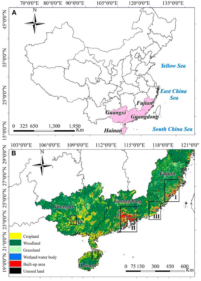
FIGURE 1. (A) Geographic situation of southeastern coastal areas in China and (B) LULC compositions in 2017. The five hotspots experiencing rapid urban expansion are identified in (B): (I) Fujian province coastal city cluster (i.e., Xiamen, Zhangzhou, and Quanzhou cities), (II) the Pearl River Delta city cluster (i.e., Guangzhou, Shenzhen, Dongguan, and Foshan cities), (III) Chao-Shan city cluster (i.e., Chaozhou, Shantou, and Jieyang cities), (IV) Nanning city in Guangxi province, and (V) Haikou city in Hainan province.

In this important agricultural production and economic development region, intensive or even excessive anthropogenic pressure (e.g., agricultural reclamation, urbanization, and deforestation), along with extreme rainfall and heterogeneous landscapes has led to severe soil erosion, which is the primary cause of land degradation (Chen Y et al., 2020; Li et al., 2020). In the past 4 decades from 1978 to 2017, the southeastern coastal area has experienced rapid economic and population growth, urban expansion, and ecosystem conservation and restoration. Furthermore, land-use transformation has been accelerated by intensive human disturbances and policy interventions, such as wetland reclamation, deforestation, revegetation projects, ecosystem restoration efforts, soil and water conservation measures, and urban landscape projects (Mao et al., 2018a; Mao et al., 2018b; Li et al., 2020; Yu et al., 2021). Land-use transitions, particularly among cropland, woodland, and built-up areas, directly alter ecosystem patterns, ES provision capacity, and potential demand (Peng et al., 2020; Wang et al., 2021; Zhang et al., 2021). In particular, urban expansions around southeastern Guangdong and Fujian provinces have degraded cropland and wetland resources, thereby threatening food and ecological security (Zhang et al., 2018; Chen et al., 2019b). Moreover, regional disparities in economic development and population growth have led to significant differentiation and spatial mismatches between the supply and demand of ESs (Peng et al., 2020; Yu et al., 2021).

2.2 Study framework and workflow

Landscape structure is closely associated with ecological processes and functions (Jean et al., 2021), and landscape composition and configuration directly alter ecological processes encompassing material and energy circulation, species migration, hydrological processes, carbon stock, and biodiversity maintenance, eventually resulting in changes in the provision capacity of ESs (Chen et al., 2019a; Chen W et al., 2020; Jean et al., 2021). In addition, human disturbances and policy interventions profoundly alter landscape composition and result in an ES imbalance (Figure 2A). For instance, population migration leads to urban expansion and increases in food and energy demands, thereby further accelerating land-use transformation among woodland, cropland, and urban areas through agricultural reclamation and deforestation practices and ultimately exacerbating the imbalance of ESs and resource scarcity. In contrast, positive policy interventions, such as ecosystem restoration projects, revegetation practices, urban landscape, and catchment management projects cause vegetation restoration and considerable changes in ecosystems, which maintain the supply capacity and enhance landscape sustainability (Yuan et al., 2019; Jiang et al., 2021a). Different landscape structures (Supplementary Figure S1) have been demonstrated to profoundly influence the material transportation, formation, and delivery of ESs (Lee et al., 2015). Specifically, the structures that are centralized, uniform, monotonous, closed, and lacking in connectivity and diversity have adverse effects on the formation and accessibility of ESs, whereas complex and diverse shapes are beneficial for biodiversity maintenance (Jean et al., 2021).

FIGURE 2

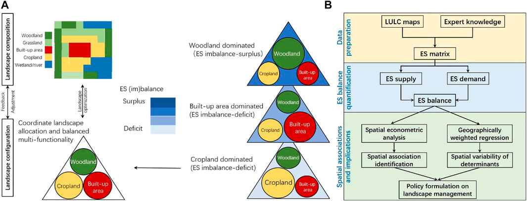
FIGURE 2. (A) Diagram of linkages between the ES balance and landscape composition and (B) study workflow. Woodlands, croplands, and built-up areas in the left column were the three dominant landscape categories, accounting for more than 90% of the total area, and were closely associated with ES supply, demand, and balance. The evolution of landscape composition and the associated ES balance are illustrated in (A) and Supplementary Figure S1.

Landscape metrics encompassing patch density (PD), landscape shape index (LSI), aggregation index, and Shannon’s diversity index (SHDI), are effective and critical indicators that reflect landscape composition, structure, shape, and fragmentation, and diversity, respectively, and have been applied worldwide in landscape planning and related fields (Mitchell et al., 2015; Ayinuer et al., 2018). For definitions and calculation formulas of landscape metrics, refer to McGarigal et al. (2012). In addition, socioeconomic variables, including population density (POPD) and gross domestic product, which indicate the intensity of human activities in the social system, also directly and indirectly respond to ESs and represent the promotion or restriction impacts of ecosystems on socioeconomic development (Wang et al., 2021; Yu et al., 2021). Thereby, we selected a group of landscape and socioeconomic variables as explanatory variables to explain the evolution of the ES balance and explore the spillover effects of spatial determinants, as presented in Figure 2B.

2.3 Datasets and methodologies

2.3.1 Data preparation

LULC datasets with a resolution of 30 × 30 m for three periods (1980, 2000, and 2017), interpreted from moderate-resolution satellite images, were derived from the Resource and Environment Data Cloud Platform (Liu et al., 2014). These datasets were produced by combining visual interpretation and machine learning techniques based on relatively high-quality images obtained from Landsat Multispectral Scanner, Thematic Mapper, Enhanced Thematic Mapper Plus, and Operational Land Imager sensors. Cross-validation through pixel checking and field validation showed that the overall accuracy for interpretation reached 92%, which is capable of capturing landscape pattern changes for regional-scale studies and has been widely applied for ecosystem assessment and ES quantification as well as in other research fields (Liu et al., 2014; Jiang et al., 2021a; Wang et al., 2021). In southeastern coastal areas as shown in Figure 1B, the first-level LULC categories encompass cropland, woodland, grassland, wetland/waterbodies, artificial surface/built-up areas, and unused land/bare land, and the second-level categories include more than 20 sub-categories; for more details on the definitions of each category and technical details for interpretation, refer to Liu et al. (2014). In addition, spatial datasets on demographic and economic attributes, with a resolution of 1 × 1 km, were derived and applied to reflect POPD and economic development changes from 1980 to 2017 (i.e., 1980, 2000, and 2017). These datasets were generated based on the significant spatial regression relationship between statistical records and nighttime stable light data derived by the Defense Meteorological Satellite Program Operational Line-scan System sensor for the years 1980–2015 (Liu et al., 2005). To avoid inconsistencies and uncertainties arising from different projection systems and spatial resolutions of LULC maps and socioeconomic indicator datasets, this study unified the coordinate and projection systems and spatial resolution (i.e., 1 × 1 km) via projection transformation and resampling tools, respectively, on ArcMap Platform (Version 10.3).

2.3.2 Quantification of ecosystem service supply–demand budget

This study applied the supply–demand budget matrix to derive the ES supply, demand, and budget indexes (ESSI, ESDI, and ESBI, respectively) of regulating, provisioning, and cultural ESs for the three time nodes over the past 4 decades. Supply and demand matrices for eighteen LULC categories and twenty-three ES categories were created on the basis of the matrix proposed and developed by Burkhard et al. (2012), Burkhard et al. (2014), with the original matrix adjusted according to expert knowledge for a specific research area (Supplementary Figure S2). The detailed process was as follows: First, because of the different LULC classification systems, we integrated the ESSI, ESDI, and ESBI proposed by Burkhard et al. (2012) by consolidating similar LULC categories. Second, more than thirty papers involving ES matrix, in particular on southern China, were collected and reviewed (e.g., Cai et al., 2017; Ou et al., 2018; Tao et al., 2018; Chen J et al., 2020; Peng et al., 2020; Jiang et al., 2021a), and the scores for entries were assigned according to these studies. The score for each entry indicates supply/demand level of individual ES, the greater is the ESSI/ESDI, the higher is the supply/demand. Then, a group of experts holding doctoral degrees, including more than 25 scholars from related fields, such as ecology, environment, hydrology, biology, and botany, of different research institutions, communities, and non-governmental organizations were requested to score matrix entries individually based on their understanding of the definitions involved in the matrix. Allowing for the relatively extensive disciplinary background, we specifically invited ten additional experts from different fields of ES research, including carbon sequestration, soil and water conservation, biodiversity conservation, climate regulation, water and soil purification, and cultural services (e.g., cultural education and recreation) for scoring. All these experts had good background knowledge and research experience in ecological, geographical, and environmental sciences in southeastern China, which guaranteed an objective and fair evaluation of criteria (Peng et al., 2020). Finally, we organized three rounds of panel discussions to reach an agreement on the final scores for the matrices. Three ES balance indexes were calculated according to the following equations:

$ESSI=\raisebox{1ex}{${\displaystyle \sum }_{v=1}^o{\displaystyle \sum }_{u=1}^p\left(A_u\times S_{uv}\right)$}\!\left/ \!\raisebox{-1ex}{${\displaystyle \sum }_{u=1}^p{A}_u$}\right.(1)$

$ESDI=\raisebox{1ex}{${\displaystyle \sum }_{v=1}^o{\displaystyle \sum }_{u=1}^p\left(A_u\times D_{uv}\right)$}\!\left/ \!\raisebox{-1ex}{${\displaystyle \sum }_{u=1}^p{A}_u$}\right.(2)$

$ESBI=\raisebox{1ex}{${\displaystyle \sum }_{v=1}^o{\displaystyle \sum }_{u=1}^p\left(A_u\times B_{uv}\right)$}\!\left/ \!\raisebox{-1ex}{${\displaystyle \sum }_{u=1}^p{A}_u$}\right.(3)$

where S_uv, D_uv, and B_uv are the supply, demand, and budget matrices, respectively, of the vth ES category of the uth LULC category; A_u represents the area of the uth LULC type; and p and o denote the number of LULC and ES categories, respectively.

2.3.3 Model for spatial spillover effects of the determinants of ecosystem service balance

We applied spatial econometric models (SECMs) to determine the associations, including spillover effects, between ESBI and drivers. Conventional econometric models (such as logistic regression and multiple regression approaches) are completely dependent on the over-idealized assumptions that suggest all involved variables are independent, stationary, and structurally stable (LeSage et al., 2009). Moreover, conventional econometric analyses rarely take the spatial correlations of independent variables into account, which results in inaccurate conclusions (Chaurasia et al., 2020). By contrast, SECMs consider the spatial associations between individual and other variables, under the premise that many socioeconomic and biophysical variables (e.g., population, trade, infrastructure, carbon emission, resource consumption, ESs, and biomass) are spatially related and closely interconnected (Cai et al., 2021). As presented in Fig. S3, the Moran’s I scatterplots of the ESBI in four provinces/region and three periods presented close correlations with the values of Moran’s I larger than 0.55, featured by spatial aggregations of ESBIs. A majority of the ESBIs concentrated in the first and third quadrants, implying that the distributions of ES deficit/surplus tend to be adjacent and spatially autocorrelated; thereby, conventional econometric analyses cannot be applied in this case. Consequently, multiple SECMs, encompassing the spatial lag model (SLM), spatial error model (SEM), and spatial Durbin model (SDM) (LeSage et al., 2009), were applied to identify the spillover effects of determinants on the ESBI. The primary formulas are expressed as follows:

$\mathit{Ln}{ESBI}_{it}=\alpha \beta \mathit{Ln}{ESBI}_{it}+{\gamma }_{i}LnX+{\gamma }_0+{\sigma }_{it}(4)$

$\mathit{Ln}{ESBI}_{it}={\gamma }_0+{\gamma }_{i}LnX+{\sigma }_{it},{\sigma }_{it}=\mu \beta \sigma +{ϵ}_{it}(5)$

$\mathit{Ln}{ESBI}_{it}=\alpha \beta \mathit{Ln}{ESBI}_{it}+{\gamma }_0+{\gamma }_{i}LnX+{\theta }_i\beta LnX+{\sigma }_{it}(6)$

where $\alpha$ means the significance of the autocorrelation of the ESBI between individual and adjacent units; LnX represents the socioeconomic and landscape variables that determine the ESBI; $\beta$ LnESBI_it and $\beta$ LnX denotes the spatial lag terms of the observation and explanatory variables, respectively (i.e., the external effect from adjacent units); $\mu$, $ϵ$_it, and $\sigma$_it are the autocorrelation, random error, and disturbance terms, respectively; $\theta$_i indicates the coefficient of $\beta$ LnX that needs to be derived; $\beta$ represents the weight matrix.

Specifically, the partial differential approach (Elhorst, 2014) was utilized to quantify the direct and indirect effects (i.e., spatial spillover effects) of the associated variables on the ESBI. Thus, the SDM is written as follows:

${ESBI}_t={\left(I_n-\alpha W\right)}^{-1}\left(X_t\gamma +W{X}_t\theta \right)+{\left(I_n-\alpha W\right)}^{-1}{\sigma }_t^{\ast }(7)$

where I_n indicates the Moran’s I index (Dall’erba, 2009) and ${\sigma }_t^{*}$ is the error term. The partial differential formula of the observation variable to the kth explanatory variable in different spatial units (X_jk for j = 1, … , M) at an individual time is written as below:

${\left[\frac{\partial ESBI}{\partial X_{1k}}\cdots \frac{\partial ESBI}{\partial X_{Nk}}\right]}_t={\left(I-\alpha W\right)}^{-1}\left[\begin{array}{ccc}{\gamma }_k& {\beta }_{12}{\theta }_k& \cdots \\ {\beta }_{21}{\theta }_k& {\gamma }_k& \cdots \\ {\beta }_{N1}{\theta }_k& {\beta }_{N2}{\theta }_k& \cdots \end{array}\begin{array}{c}{\beta }_{1N}{\theta }_k\\ {\beta }_{2N}{\theta }_k\\ {\gamma }_k\end{array}\right](8)$

The diagonal and the row or column of the non-diagonal terms reflect the direct and indirect effects of the explanatory variables on the ESBI, respectively. The former and latter represent the effects of changes in an explanatory variable on the ESBI in individual and adjacent units, respectively (Meng et al., 2021).

2.3.4 Model comparison and validation

To examine the effects of spatiotemporal variation (i.e., heterogeneity) of independent variables on dependent variables, the geographically and temporally weighted regression (GTWR) approach (Fotheringham et al., 1998; He and Huang, 2018) was used to identify the spatiotemporal associations between the ES supply–demand budget and socioeconomic and landscape variables (Cai et al., 2021). The fundamental formulas are as follows:

$Y_i={\alpha }_0\left(u_i,v_i\right)+{\displaystyle \sum }_{j=1}^m{\alpha }_j\left(u_i,v_i\right)x_{ij}+{\delta }_i(9)$

${\alpha }_j\left(u_i,v_i\right)={\left(M^{T}V\left(u_i,v_i\right)M\right)}^{-1}{M}^{T}V\left(u_i,v_i\right)y_i(10)$

where Y_idenotes the dependent variable (i.e., ESBI); α₀ (u_i, v_i) and α_j denote the intercept and regression coefficient for variable j in county i, respectively; (u_i, v_i) represents the coordinates of the geographic center of gravity; m is the number of explanatory variables; δ_i is a residual term; M and M^T are the independent variables and transposed matrixes, respectively; V (u_i, v_i) is the spatial weight matrix. As shown in Supplementary Table S1, in contrast to ordinary least squares and GWR, GTWR performs better in capturing the effects of spatiotemporal heterogeneity in independent variables, because the overall assessment results, indicated by R², of GTWR for three periods are larger than those of the other two models.

To minimize the effect of the multicollinearity of independent variables (i.e., landscape metrics and socioeconomic variables) on spatial econometric analyses, this study tested the multicollinearity before linear regression through the variance inflation factor (VIF; Zheng, 1995), which denotes the possibility of collinearity between explanatory variables. The calculation formula for VIF is expressed as follows:

$VIF=\frac{1}{1-r_i^2}(11)$

where r_i represents the coefficient of correlation between the independent variable i and the other explanatory variables. When the VIF is less than 10, multicollinearity does not significantly influence the performance of the regression model. As shown in Table 1, the VIF values were less than 10, indicating that multicollinearity did not exist between the explanatory variables.

TABLE 1

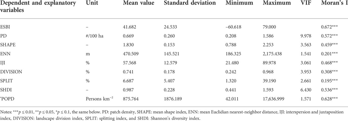
TABLE 1. Summaries of the ESBI and explanatory variables for 1980, 2000, and 2017.

3 Results

3.1 Landscape dynamics and evolution of the ecosystem service supply–demand budget

In the three time nodes of 1980, 2000, and 2017, the overall patterns of landscape composition in the four provinces/region remained stable, except for some hotspots of rapid urban expansion (Figure 3). The narrow coastal zone of Fujian province experienced rapid land-use transformation from croplands, including agricultural ponds and wetlands, to urban areas (Figure 3A). In Guangdong province, the two large urban agglomerations around the northeast and southeast along the coastal area (Chao-Shan and the Pearl River Delta city clusters in Figure 1B) also expanded rapidly, which accelerated the loss of wetlands and agricultural ponds, particularly of mangrove, coral reef, beach, and intertidal zone in the Pearl River Delta city cluster (Figure 3B). In contrast to those in Fujian and Guangdong, the urbanizing trends of Zones III and IV were not as significant as those of Zones I and II, and Nanning city and Haikou city were situated in the inland and coastal regions, respectively (Figures 3C,D). Similarly, the landscape metrics remained stable for the overall patterns of the three periods (Fig. S4), and substantial landscape changes were identified in coastal hotspots of urbanization.

FIGURE 3

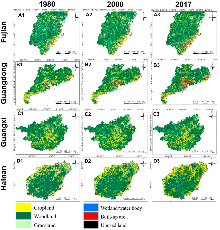
FIGURE 3. Spatial disparities of landscape composition for four provinces/region in the three periods of 1980, 2000, and 2017: (A) Fujian, (B) Guangdong, (C) Guangxi, and (D) Hainan.

The ES balance patterns, including the ESSI, ESDI, and ESBI, presented similar patterns as that of landscape composition (Figure 4): the high ESSIs were mainly spatially concentrated in woodlands and grasslands in inland areas, whereas the coastal areas were characterized by strong ES demands (i.e., ESDIs), particularly for rapidly expanding areas. Accordingly, the high and low ESBI values (i.e., ES surplus and deficit, respectively) were situated in the inland and coastal regions, respectively. Specifically, this study focused on the four hotspots of rapid expansion and investigated the temporal changes in the three ES balance indexes (Figure 5). All the ESBIs in the four zones declined substantially, and the different categories of ESs and total ESs presented increasingly strong demands and weak supply capacity (i.e., high ESDIs and low ESSIs, respectively).

FIGURE 4

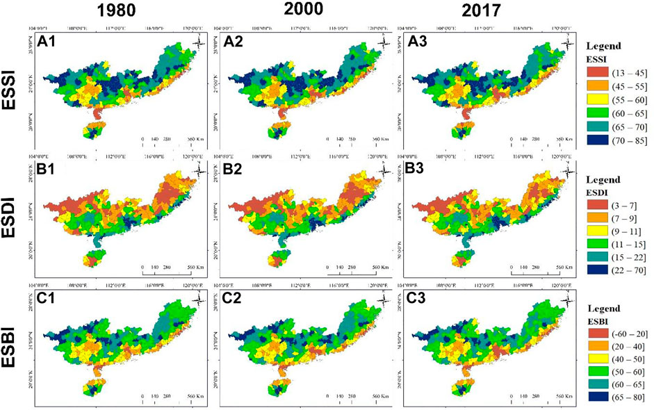
FIGURE 4. Spatial evolution of the (A) ESSI, (B) ESDI, and (C) ESBI of the south-eastern coastal region of China for the three periods of 1980, 2000, and 2017.

FIGURE 5

FIGURE 5. Temporal changes in the ESBI and supply and demand of total ESs and different categories of ESs in five hotspots of rapid urbanization. Blue, green, and red lines represent the budget index, supply, and demand of ESs, respectively. For geographic locations of rapidly urbanizing regions, refer to Figure 1B.

3.2 Spatial associations between the ecosystem service supply–demand budget and landscape structure

As shown in Figure 6, the ES balance indexes were significantly correlated with landscape composition (p < 0.0001). The proportions of woodlands and grasslands were positively correlated with ESSI and ESBI but negatively correlated with ESDI. In contrast, both ESSIs and ESDIs in cropland and urban areas presented downward and upward trends, respectively, with increasing proportions, reflecting that woodland and grassland had relatively high ES supply capacities, whereas urban area and cropland presented strong ES demands.

FIGURE 6

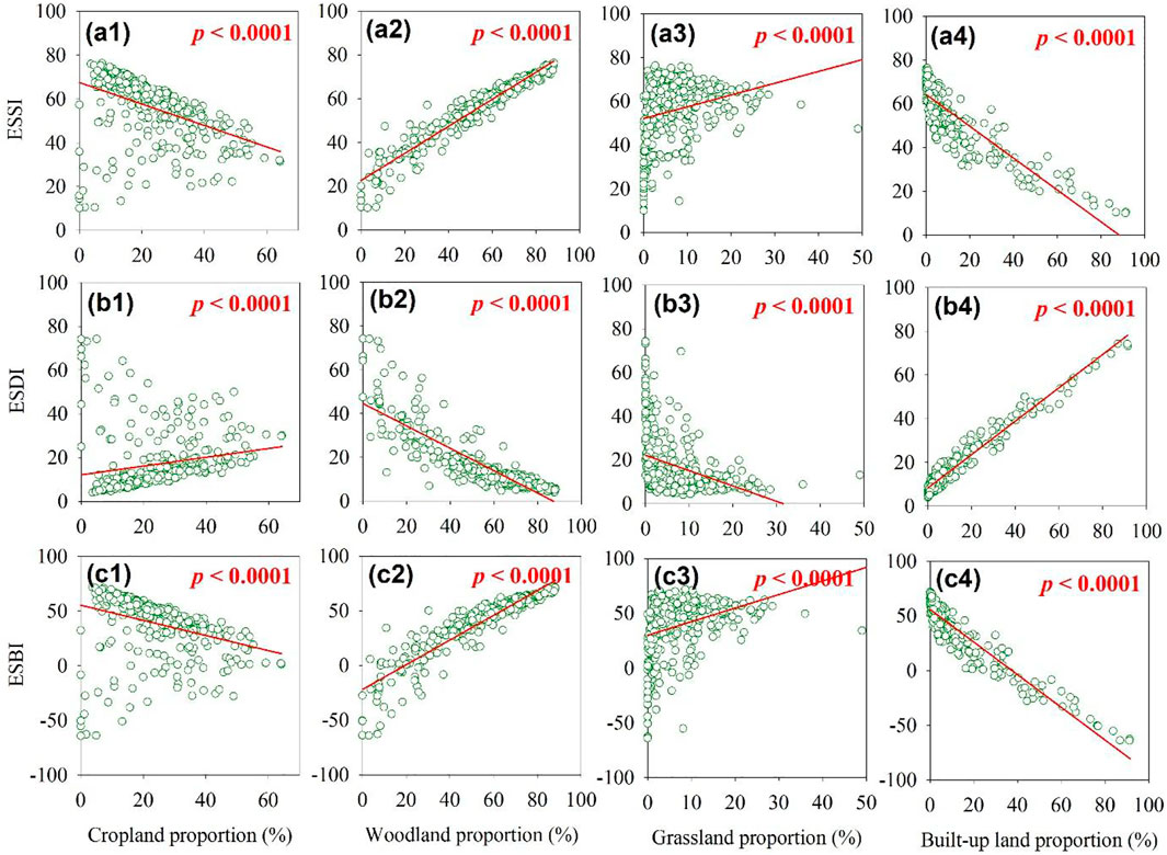
FIGURE 6. Associations between (A) ESSI, (B) ESDI, and (C) ESBI and dominant landscape compositions.

In addition to landscape composition, landscape metrics were also significantly related to ES balance indexes (Figures 7, 8). The number of patches (NP), landscape shape index (LSI), and patch cohesion index (COHESION) were positively correlated with the ESSI, whereas the other metrics presented negative correlations, all of which reached the p = 0.0001 significance level. The ESBI also showed a similar correlation with landscape metrics, and positive correlations were observed only in NP, LSI, and COHESION. Both ESSI and ESBI were negatively correlated with POPD, which indicated that population growth weakened ES supply and exacerbated ES imbalance.

FIGURE 7

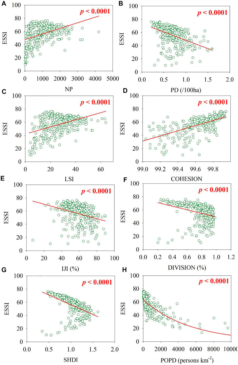
FIGURE 7. Associations between the ESSI and landscape and socioeconomic variables: (A) NP, (B) PD, (C) LSI, (D) COHESION, (E) IJI, (F) DIVISION, (G) SHDI, and (H) POPD.

FIGURE 8

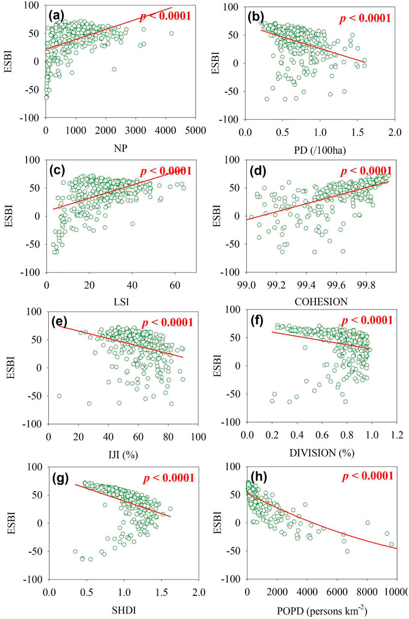
FIGURE 8. Associations between the ESBI and landscape and socioeconomic variables: (A) NP, (B) PD, (C) LSI, (D) COHESION, (E) IJI, (F) DIVISION, (G) SHDI, and (H) POPD.

SECMs revealed that observation and explanatory variables (i.e., ESBI and associated variables) were significantly correlated, but the regression coefficients in the different models with spatial and time-period fixed effects (STFEs) were different (Table 2). For example, in the SLM and SEM with STFEs and SDM with spatial fixed effects (SFEs), PD, ENN, and SHDI made positive contributions to the ESBI, whereas SHAPE, IJI, and DIVISION negatively contributed to the ESBI; almost all the regressions reached a significance level of p = 0.01. In the SDM with time-period fixed effects (TFEs), the regression coefficients of PD, SHAPE, ENN, and SHDI were opposite to those in the other models, including SLM, SEM, and SDM with SFEs and SDM with STFEs. In addition, the GTWR revealed that the spatial determinants of ESBI showed strong variability (Supplementary Figure S5), which depended on the dominant effects of the landscape metrics for specific regions.

TABLE 2

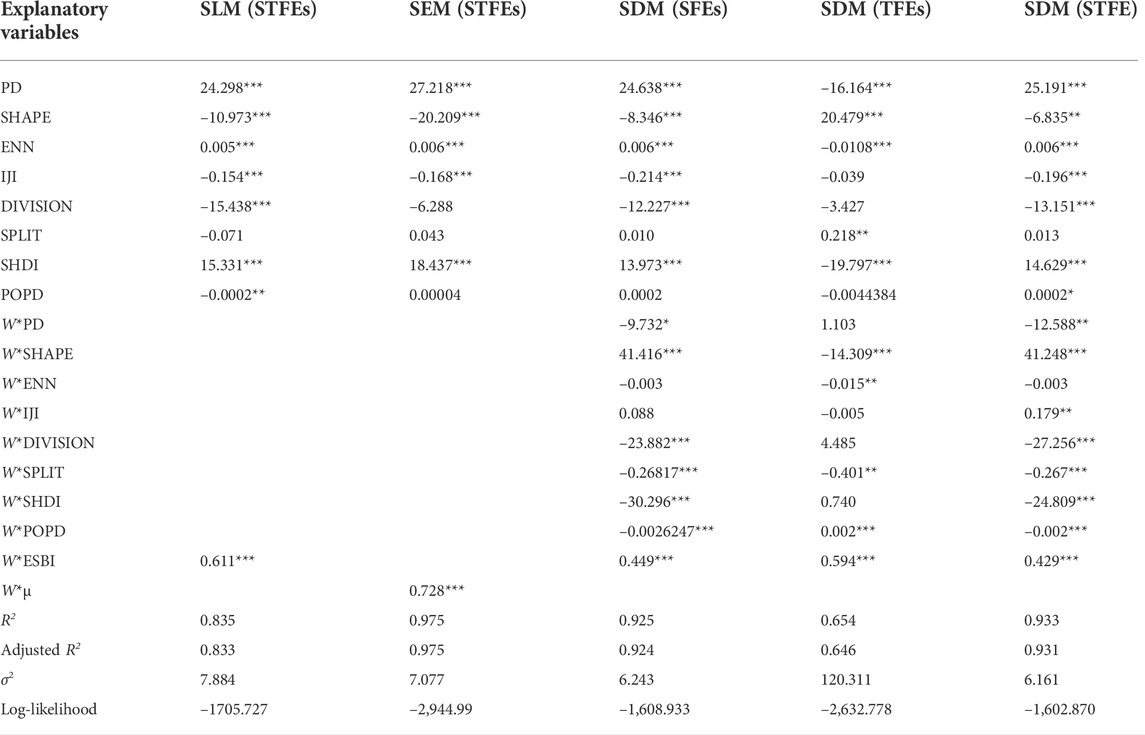
TABLE 2. Spatial associations between the ESBI and explanatory variables quantified using the SECMs.

The direct, indirect, and total effects of the explanatory variables on ESBIs in local and adjacent locations are listed in Table 3. Direct and indirect effects mean the impact of explanatory variables from local and adjacent locations, respectively. In the SDM, almost all explanatory variables were statistically significant in the regression analyses. For example, the direct and indirect effects (spillover effects) of SHDI were 15.340 and 10.274, respectively, indicating that an increase in SHDI in individual areas resulted in an increase in the ESBI in local and adjacent locations.

TABLE 3

TABLE 3. Direct and indirect effects of explanatory variables on the ESBI quantified using the SDM.

4 Discussion

4.1 Spatial determinants of the ecosystem service supply–demand budget

Significant spatial associations between ES balance and explanatory variables embody the importance of landscape metrics in describing spatial composition and configuration, which are associated with ecological, hydrological, and other biophysical and biogeochemical processes (Mitchell et al., 2015; Jean et al., 2021). Specifically, landscape dynamics driven by human disturbances and policy interventions, for instance, urbanization, terrain reconstruction, revegetation projects, and soil and water conservation measures, might prevent or disturb material circulation and energy transportation and further influence the formation of ESs, such as soil erosion control, hydrological and climatic regulations, and species migration (Jean et al., 2021). For instance, PD reflects landscape fragmentation and intensity of human interventions (McGarigal et al., 2012; Ayinuer et al., 2018). Normally, the areas that feature high human activities are located in urban areas, which have strong demands and low provision capacity of ESs (Peng et al., 2020; Zhang et al., 2021); thus, PD negatively correlates with the ESSI and ESBI (Figures 7, 8). The LSI represents the complexity of patches, and the positive correlation between LSI and ESSI (ESBI) demonstrates that the more irregular the patches are, the smaller the ESBI is. Identifying the spatial relationship between landscape structure and the ES supply–demand balance deepens our understanding of the impact of landscape composition and structure on this balance, which further supports landscape planning and management by monitoring landscape dynamics and optimizing the critical landscape composition and configuration (Mitchell et al., 2015; Chen et al., 2019a; Chen W et al., 2020).

In addition, spatial econometric analyses concluded that neither landscape metrics nor socioeconomic variables are the sole driving factors of ES balance; thus, these factors should be concurrently considered as critical determinants in landscape planning and ES management (Jiang et al., 2020; Yu et al., 2021). The significantly negative correlations (p < 0.0001) between ESBI and POPD demonstrated that population growth resulted in a rapid increase in the demand for food, water, energy, and land resources, and ESs, which further promoted land-use transitions, altered supply and demand patterns, and challenged the ES balance (Wang et al., 2021).

Traditional econometric models assume that observation and explanatory variables are spatially independent, whereas geographic location-based variables are typically spatially correlated, and that this spatial characteristic should be carefully considered in regression analyses to reduce inaccurate results (Meng et al., 2021). Spatial econometric analyses consider spatial dependence and spillover effects, which improves the interpretability of spatial autocorrelations and demonstrates that SECMs can be adopted as useful tools to identify the determinative variables of ES budgets (Chen W et al., 2020; Cai et al., 2021; Meng et al., 2021). In addition, GTWR analysis revealed that the primary determinants presented strong spatial heterogeneity in influencing the patterns of supply–demand balance (Supplementary Figure S5), which has also been proved in existing literatures (e.g., Ayinuer et al., 2018; Funes et al., 2019). Landscape planning should allow for spatial variations in critical landscape metrics according to specific locations and formulation of localized and flexible, but not monotonous, policy interventions to optimize the regional landscape and ensure ES balance.

4.2 Implications of research findings for landscape planning and ecosystem service management

Incorporating ES supply and demand perspectives into ES assessment provides a complete and clear understanding of ecosystem evolution and ES dynamics and supports practical benefits for landscape optimization, ES management, and ecosystem conservation (Chen W et al., 2020). Revealing the ES surplus and deficit enables us to understand the impacts of human activity-driven landscape changes on ESs and identify regions that suffer from ES scarcity, and therefore, are not suitable for future exploitation. Furthermore, ES balance indexes can be used as effective indicators or policy tools to direct landscape planning and decisions (Yuan et al., 2019; Jiang et al., 2021a; Zhang et al., 2021).

SECMs identified the primary determinants of ES supply–demand balance and found that landscape composition, fragmentation, shape, and complexity were closely correlated with the ES balance. These determinants should be considered in landscape planning and land-use allocation, particularly for green and blue infrastructure in rapidly expanding urban agglomerations and coastal areas experiencing intensive exploitation. For instance, as shown in Figures 9A–D, the case of Guangzhou city (i.e., one of the city clusters in Zone II of Figure 1B) demonstrated that local environmental management and landscape planning already considered green and blue spaces as important components of urban ecosystems and reserved some spaces for rivers, lakes, forests, grasslands, and wetlands (Mao et al., 2018a; Mao et al., 2018b). These components generate crucial ESs such as air and water purification, climatic regulation, and cultural services, including education, tourism, and recreation (Zhang et al., 2021). However, the spatial allocation of these landscape patches is still not completely appropriate. For instance, one of the most important functions of green and blue spaces in urban agglomerations is to mitigate the heat island effect through the cooling effect of woodlands, grasslands, and wetlands (Liu et al., 2021). However, the parallel distribution of different landscape categories shown in Supplementary Figure S1A4–A5 is not beneficial for heat transportation and air temperature regulation (Zhang et al., 2021). In addition, the concentration and distribution of urban areas (Supplementray Figure S1A1–A3) do not sufficiently allow for the connectivity and diversity of landscape patches and constitute adverse conditions for material transportation, species migration, and delivery of other ESs (Mitchell et al., 2015). Therefore, the diversity, connectivity, and appropriate combination of different landscape categories should be maintained, reallocated, and optimized from the perspective of ES balance and landscape multifunctionality (Supplementray Figure S1A6); Chen W et al., 2020; Sun et al., 2020). However, considering the negative correlations between landscape fragmentation and the ESBI (Figure 8), the patches should be maintained as relatively complete because excessive fragmentation cannot facilitate the maintenance of ES balance.

FIGURE 9

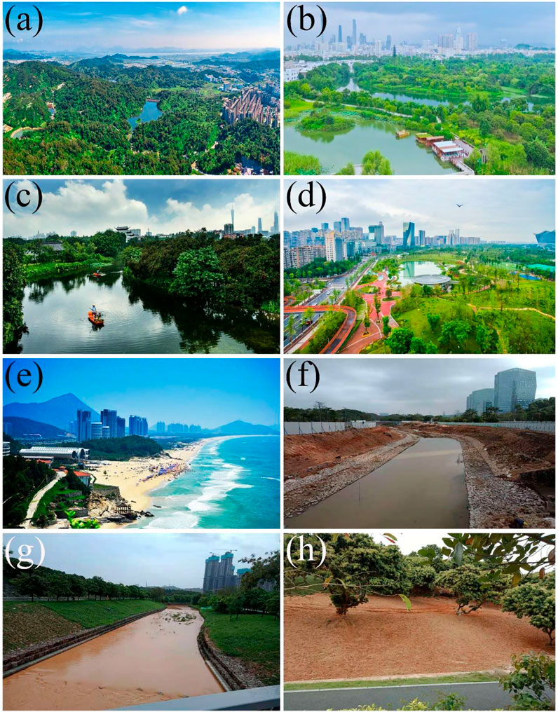
FIGURE 9. (A–D) Pictures of urban landscape compositions coordinating blue and green infrastructures (i.e., wetlands, rivers, lakes, woodlands, and grasslands) and urban development, (E) coastal exploitation, and (F–H) inappropriate urban landscape and catchment management projects that damage surface vegetation cover and exacerbate soil loss and water pollution. (A and B), (C and D), and (E) are from the Haizhu and Liwan districts of Guangzhou city and Jieyang city of Guangdong province, respectively. (F and H) Are from the Nanshan District of Shenzhen city, Guangdong province.

Specifically, considering the distinctive environmental, socioeconomic, and industrial features of coastal cities, landscape planning and regional development for these areas should conserve and appropriately allocate important landscape elements according to their ecological benefits to maintain regional ES balance and enhance ecosystem sustainability. For instance, coastal mangroves and coral reefs typically have important ecological functions, such as the mitigation of geological and meteorological disasters caused by tsunamis and typhoons (Ren et al., 2019). In addition, the wetland and mangrove ecosystems in urban–rural transition zones primarily support material and energy cycles and exhibit important ESs, such as heat island effect mitigation and aquatic purification (Jia et al., 2018). However, commercial exploitation and other inappropriate practices such as mangrove deforestation for aquaculture ponds as well as agricultural pond and wetland losses caused by urbanization and development of tourism industry normally destroy ecosystems, which further weakens ESs and might lead to irreversible damage (Mao et al., 2018a; Mao et al., 2018b; Ren et al., 2019). Therefore, coastal wetlands, mangroves, and coral reefs should be carefully conserved from the perspective of ecosystem connectivity, diversity, and functionality, and their excessive exploitation for commercial purposes and economic benefits, such as by tourism and real estate industries, should be avoided.

Results of the spatial regression analysis shown in Table 3 indicate that the ES balance in specific locations is associated with the ES balance in adjacent regions because of the existence of spatial spillover effects. The underlying explanation is that a specific landscape category is more likely to be converted to another category if it is adjacent to a location that has been converted (Jiang et al., 2020; Cai et al., 2021). Similarly, population growth and economic development in developed regions tend to provide economic benefits and environmental pressures to neighboring regions (Chi and Ho, 2018; Jiang et al., 2020). Urban sprawl and population pressure result in increased energy, resource, and ES demands, which in turn lead to the degradation of the ecosystem and deterioration of the ES balance (Baró et al., 2016; Zhang et al., 2021). To expand the production scale, increase economic profits, and fulfill the requirements of resources and ESs, industries and enterprises that have high resources and ES demands tend to shift from local counties with considerable environmental constraints to adjacent regions with sufficient ES supplies and fewer resource constraints. Thus, the landscape and socioeconomic variables in local areas not only determine the ES balance in local areas but also influence the ES balance in their surrounding regions (Chen et al., 2019a; Chen W et al., 2020). Specifically, spillover effects are clearly presented in urban landscape projects, including catchment governance and soil erosion control (Figures 9F–H). Although landscape projects in downstream ecosystems have improved land surface vegetation cover (Figure 9G), the soil loss-induced water pollution in upstream regions has not been effectively mitigated; thus, river channel sedimentation downstream is still severe (Figures 9F,H).

This study revealed the determinants of ES balance and their spillover effects, implying that, in addition to effective efforts by individual local communities to conserve ecosystems and maintain ES balance, strengthening coordination and collaborative efforts are also required from adjacent areas for them to move from being ES supply sources to beneficiaries (Chen et al., 2019a; Jiang et al., 2021a; Jean et al., 2021).

4.3 Uncertainties, limitations, and future perspectives

Some uncertainties and limitations remain in the current study. The current supply–demand matrix proposed by Burkhard et al. (2012), Burkhard et al. (2014) and adapted based on semi-quantitative local expert knowledge might not completely reflect the actual conditions of the research areas, and hence, it should be further refined and adapted according to other natural environmental conditions and socioeconomic features, including climate, terrain, vegetation species, and industrial and economic levels (e.g., Lorencová et al., 2016; Carli et al., 2018; Barbieri and Consoli, 2019; Raza et al., 2019). Existing studies have adopted an expert knowledge approach to quantify social demands for the assessment of ES balance, particularly for the demand aspect (e.g., Campagne et al., 2018; Tao et al., 2018; Sun et al., 2020). As the scoring method is based on subjective experience and it largely does not rely on accurate input parameters and complex data requirements, it can only reflect the relative levels of supply and demand (Burkhard et al., 2014). In addition, the ES demands of each era are different, and their values also differ over decades with the development of socioeconomic conditions (Carli et al., 2018; Barbieri and Consoli, 2019), and thus, it is not completely reasonable to apply the present assessment standards (as shown in Fig. S2) to assess the ES balance in previous decades. Therefore, in future studies, more input data from various sources, such as statistical records and spatially explicit data, should be incorporated into the assessment to obtain more accurate results and absolute values of ES demand (Schirpke et al., 2019; Yuan et al., 2019; Wang et al., 2021). Allowing for the low data accessibility of county-scale socioeconomic and environmental variables (Blanco et al., 2017), this study recommends exploring the possibilities of applying various emerging spatial mobile data to assess sub-county, site, and pixel-scale ES demands (Funes et al., 2019; Liu et al., 2020).

The GTWR and Moran’s I scatterplots showed that the supply–demand balance and its determinants exhibited significant spatial autocorrelations and heterogeneity and might largely rely on research scales. Some studies also show that interactions among ESs are complicated because of scale effects (Kim and Arnhold, 2018; Wilkerson et al., 2018). Therefore, the current county-scale analysis and its conclusions might not be applicable to land-use management at different levels of governments, and hence, further studies should be conducted to reveal the impacts of landscape structure on ES balance at different spatial scales and to practically support strategy formulation and implementation for combating ecosystem degradation. In terms of spillover effects, this study only obtained the direct and indirect effects of explanatory variables through SECMs (Table 3), and therefore, the effects of LULC transformation and socioeconomic indicator change in specific units on the ES balance at a regional scale is still not clear. The mechanisms of influence on the ES balance can be revealed by spatially explicit models, such as Integrated Valuation of Ecosystem Services and Trade-offs (Sharp et al., 2018) and Artificial Intelligence for Ecosystem Services (Villa et al., 2009) that couple landscape composition and structure with ESs in an integrated manner. The driving mechanisms, delivery process, and spatial variation of ES supply and demand must be investigated by including more involved socioeconomic indicators (e.g., transport network and road density) for the formulation of practical solutions toward sustainable landscape management (Wilkerson et al., 2018; Schirpke et al., 2019).

5 Conclusion

A coastal area in southeastern China was selected as a case study to reveal the spatial patterns of ES supply–demand budget in 1980, 2000, and 2017 by applying the supply–demand matrix. We identified the spatial determinants and heterogeneity of the ES budget using SECMs and GWR approaches. The overall patterns of ES balance in three time nodes were stable, whereas ES deficits typically existed in rapidly urbanizing areas. ESSI and ESBI closely correlated with landscape proportions because cropland and built-up areas exhibited week ES supply and strong ES demand, while woodland and grassland had strong ES supply and week ES demand. Landscape variables and POPD were identified as the primary spatial determinants of the ES balance and they were closely associated with the ESBI and exhibited remarkable spatial variability and external effects.

The spatial heterogeneity of determinants implies that regional landscape management strategies should account for the spatial dependencies of independent variables and provide an important reference for decision-making for regional landscape planning and ecosystem conservation. In addition, localized biophysical and socioeconomic variables, such as landscape composition, environmental conditions, economic levels, and localized management practices, which are designed according to actual conditions, should be considered to accurately assess and effectively reconcile ES imbalance (i.e., ES deficits) through targeted policy regulations, landscape optimizations, and other human interventions. Considering the existence of spatial spillover effects of determinants, the strategy formulation and solution implementation for landscape planning and ES management should not completely rely on individual governments or organizations but rather require collaborative efforts from different levels of communities in both local and adjacent districts (i.e., cross-border regions), particularly for the rapidly expanding coastal urban agglomerations.

Data availability statement

The original contributions presented in the study are included in the article/Supplementary Material, further inquiries can be directed to the corresponding author.

Author contributions

WC and CJ: Conceptualization, Methodology, Writing “original draft, Writing” review and editing. YW: Investigation, Methodology, Data curation. XL, BD, JY, and WH: Funding acquisition, Project administration, Resources.

Acknowledgments

Guangdong Academy of Sciences Project of Science and Technology Development (2020GDASYL-20200103010), National Natural Science Foundation of China (41901258; 41976189; 42006170; 42101084), Guangdong Forestry Science and Technology Project (2020KJCX003), Provincial Science and Technology Program of Guangdong Province (2019B020208002), Marine Economy Development Foundation of Guangdong Province (No. GDNRC[2020]051), Natural Science Foundation of Guangdong Province (2022A1515011898), and National Park Construction Project (2021GJGY029).

Conflict of interest

The authors declare that the research was conducted in the absence of any commercial or financial relationships that could be construed as a potential conflict of interest.

Publisher’s note

All claims expressed in this article are solely those of the authors and do not necessarily represent those of their affiliated organizations, or those of the publisher, the editors and the reviewers. Any product that may be evaluated in this article, or claim that may be made by its manufacturer, is not guaranteed or endorsed by the publisher.

Supplementary material

The Supplementary Material for this article can be found online at: https://www.frontiersin.org/articles/10.3389/fenvs.2022.1002902/full#supplementary-material

References

Ayinuer, Y., Zhang, F., Yu, H., and Kung, H. (2018). Quantifying the spatial correlations between landscape pattern and ecosystem service value: a case study in ebinur lake basin, xinjiang, China. Ecol. Eng. 113, 94–104. doi:10.1016/j.ecoleng.2018.02.005

CrossRef Full Text | Google Scholar

Barbieri, N., and Consoli, D. (2019). Regional diversification and green employment in US metropolitan areas. Res. Policy 48, 693–705. doi:10.1016/j.respol.2018.11.001

CrossRef Full Text | Google Scholar

Baró, F., Palomo, I., Zulian, G., Vizcaino, P., Haase, D., and Gómez-Baggethun, E. (2016). Mapping ecosystem service capacity, flow and demand for landscape and urban planning: a case study in the barcelona metropolitan region. Land Use Policy 57, 405–417. doi:10.1016/j.landusepol.2016.06.006

CrossRef Full Text | Google Scholar

Blanco, V., Holzhauer, S., Brown, C., Lagergren, F., Vulturius, J., Lindeskog, M., et al. (2017). The effect of forest owner decision-making, climatic change and societal demands on land-use change and ecosystem service provision in Sweden. Ecosyst. Serv. 23, 174–208. doi:10.1016/j.ecoser.2016.12.003

CrossRef Full Text | Google Scholar

Burkhard, B., Kroll, F., Nedkov, S., and Müller, F. (2012). Mapping ecosystem service supply, demand and budgets. Ecol. Indic. 21, 17–29. doi:10.1016/j.ecolind.2011.06.019

CrossRef Full Text | Google Scholar

Burkhard, B., Kandziora, M., Hou, Y., and Müller, F. (2014). Ecosystem service potentials, flows and demands concepts for spatial localisation, indication and quantification. Landsc. Online 34, 1–32. doi:10.3097/lo.201434

CrossRef Full Text | Google Scholar

Cai, W., Gibbs, D., Zhang, L., Ferrier, G., and Cai, Y. (2017). Identifying hotspots and management of critical ecosystem services in rapidly urbanizing Yangtze River Delta Region, China. J. Environ. Manage. 191, 258–267. doi:10.1016/j.jenvman.2017.01.003

PubMed Abstract | CrossRef Full Text | Google Scholar

Cai, Z., Li, W., and Cao, S. (2021). Driving factors for coordinating urbanization with conservation of the ecological environment in China. Ambio 50, 1269–1280. doi:10.1007/s13280-020-01458-x

PubMed Abstract | CrossRef Full Text | Google Scholar

Campagne, C. S., Roche, P. K., and Salles, J.-M. (2018). Looking into pandora’s box: ecosystem disservices assessment and correlations with ecosystem services. Ecosyst. Serv. 30, 126–136. doi:10.1016/j.ecoser.2018.02.005

CrossRef Full Text | Google Scholar

Carli, R., Dotoli, M., and Pellegrino, R. (2018). Multi-criteria decision-making for sustainable metropolitan cities assessment. J. Environ. Manage. 226, 46–61. doi:10.1016/j.jenvman.2018.07.075

PubMed Abstract | CrossRef Full Text | Google Scholar

Castillo-Eguskitza, N., Martín-Lopez, ´ B., and Onaindia, M. (2018). A comprehensive assessment of ecosystem services: integrating supply, demand and interest in the urdaibai biosphere reserve. Ecol. Indic. 93, 1176–1189. doi:10.1016/j.ecolind.2018.06.004

CrossRef Full Text | Google Scholar

Chaplin-Kramer, R., Sharp, R. P., Weil, C., Bennett, E. M., Pascual, U., Arkema, K. K., et al. (2019). Global modeling of nature’s contributions to people. Science 366 (6462), 255–258. doi:10.1126/science.aaw3372

PubMed Abstract | CrossRef Full Text | Google Scholar

Chaurasia, H., Srivastava, S., and Singh, J. K. (2020). Does seasonal variation affect diarrhoea prevalence among children in India? An analysis based on spatial regression models. Child. Youth Serv. Rev. 118, 105453. doi:10.1016/j.childyouth.2020.105453

CrossRef Full Text | Google Scholar

Chen, W., Chi, G., and Li, J. (2019a). The spatial association of ecosystem services with land use and land cover change at the county level in China, 1995–2015. Sci. Total Environ. 669, 459–470. doi:10.1016/j.scitotenv.2019.03.139

PubMed Abstract | CrossRef Full Text | Google Scholar

Chen, W., He, B., Nover, D., Lu, H., Liu, J., Sun, W., et al. (2019b). Farm ponds in southern China: Challenges and solutions for conserving a neglected wetland ecosystem. Sci. Total Environ. 659, 1322–1334. doi:10.1016/j.scitotenv.2018.12.394

PubMed Abstract | CrossRef Full Text | Google Scholar

Chen, J., Xiao, H., Li, Z., Liu, C., Ning, K., and Tang, C. (2020). How effective are soil and water conservation measures (SWCMs) in reducing soil and water losses in the red soil hilly region of China? A meta-analysis of field plot data. Sci. Total Environ. 735, 139517. doi:10.1016/j.scitotenv.2020.139517

PubMed Abstract | CrossRef Full Text | Google Scholar

Chen, W., Chi, G., and Li, J. (2020). The spatial aspect of ecosystem services balance and its determinants. Land Use Policy 90, 104263. doi:10.1016/j.landusepol.2019.104263

CrossRef Full Text | Google Scholar

Chen, Y., Dong, J., Xiao, X., Ma, Z., Tan, K., Melville, D., et al. (2020). Effects of reclamation and natural changes on coastal wetlands bordering China's Yellow Sea from 1984 to 2015. Land Degrad. Dev. 30, 1533–1544. doi:10.1002/ldr.3322

CrossRef Full Text | Google Scholar

Chi, G., and Ho, H. C. (2018). Population stress: a spatiotemporal analysis of population change and land development at the county level in the contiguous United States, 2001-2011. Land Use Policy 70, 128–137. doi:10.1016/j.landusepol.2017.10.008

PubMed Abstract | CrossRef Full Text | Google Scholar

Costanza, R., de Groot, R., Braat, L., Kubiszewski, I., Fioramonti, L., Sutton, P., et al. (2017). Twenty years of ecosystem services: how far have we come and how far do we still need to go? Ecosyst. Serv. 28, 1–16. doi:10.1016/j.ecoser.2017.09.008

CrossRef Full Text | Google Scholar

Dall’erba, S. (2009). “Exploratory spatial data analysis,” in International encyclopedia of human geography (Cham: Springer), 683–690. doi:10.1016/B978-008044910-4.00433-8

CrossRef Full Text | Google Scholar

Elhorst, J. P. (2014). MATLAB software for spatial panels. Int. Reg. Sci. Rev. 37 (3), 389–405. doi:10.1177/0160017612452429

CrossRef Full Text | Google Scholar

Fotheringham, A. S., Brundson, C., and Charlton, M. (1998). Geographically weighted regression: A natural evolution of the expansion method for spatial data analysis. Environ. Plan. A 30, 1905–1927. doi:10.1068/a301905

CrossRef Full Text | Google Scholar

Funes, I., Savé, R., Rovira, P., Molowny-Horas, R., Alcañiz, J. M., Ascaso, E., et al. (2019). Agricultural soil organic carbon stocks in the north-eastern iberian peninsula: drivers and spatial variability. Sci. Total Environ. 668, 283–294. doi:10.1016/j.scitotenv.2019.02.317

PubMed Abstract | CrossRef Full Text | Google Scholar

He, Q. Q., and Huang, B. (2018). Satellite-based mapping of daily high-resolution ground PM2.5 in China via space-time regression modeling. Remote Sens. Environ. 206, 72–83. doi:10.1016/j.rse.2017.12.018

CrossRef Full Text | Google Scholar

Jean, P. M., Jaramar, V. R., Andrés, F. S. C., Sofía, L. C., Adrian, G. C., Rebecca, K. R., et al. (2021). Considering landscape-level processes in ecosystem service assessments. Sci. Total Environ. 796, 149028. doi:10.1016/j.scitotenv.2021.149028

PubMed Abstract | CrossRef Full Text | Google Scholar

Jia, M., Wang, Z., Zhang, Y., Mao, D., and Wang, C. (2018). Monitoring loss and recovery of mangrove forests during 42 years: The achievements of mangrove conservation in China. Int. J. Appl. Earth Obs. Geoinf. 73, 535–545. doi:10.1016/j.jag.2018.07.025

CrossRef Full Text | Google Scholar

Jiang, C., Zhao, L., Dai, J., Liu, H., Lie, Z., Wang, X., et al. (2020). Examining the soil erosion responses to ecological restoration programs and landscape drivers: A spatial econometric perspective. J. Arid. Environ. 183, 104255. doi:10.1016/j.jaridenv.2020.104255

CrossRef Full Text | Google Scholar

Jiang, C., Yang, Z., Wen, M., Huang, L., Liu, H., Wang, J., et al. (2021a). Identifying the spatial disparities and determinants of ecosystem service balance and their implications on land use optimization. Sci. Total Environ. 793, 148472. doi:10.1016/j.scitotenv.2021.148472

PubMed Abstract | CrossRef Full Text | Google Scholar

Jiang, C., Yang, Z., Wang, X., Dong, X., Li, Z., and Li, C. (2021b). Examining the reversal of soil erosion decline in the hotspots of sandstorms: A non-linear ecosystem dynamic perspective. J. Arid. Environ. 186, 104421. doi:10.1016/j.jaridenv.2020.104421

CrossRef Full Text | Google Scholar

Kim, I., and Arnhold, S. (2018). Mapping environmental land use conflict potentials and ecosystem services in agricultural watersheds. Sci. Total Environ. 630, 827–838. doi:10.1016/j.scitotenv.2018.02.176

PubMed Abstract | CrossRef Full Text | Google Scholar

Larondelle, N., and Lauf, S. (2016). Balancing demand and supply of multiple urban ecosystem services on different spatial scales. Ecosyst. Serv. 22, 18–31. doi:10.1016/j.ecoser.2016.09.008

CrossRef Full Text | Google Scholar

Lee, Y., Ahern, J., and Yeh, C. (2015). Ecosystem services in peri-urban landscapes: the effects of agricultural landscape change on ecosystem services in taiwan’s Western coastal plain. Landsc. Urban Plan. 139, 137–148. doi:10.1016/j.landurbplan.2015.02.023

CrossRef Full Text | Google Scholar

LeSage, J., Pace, R., Schucany, W., Schilling, E., and Balakrishnan, N. (2009). Introduction to spatial econometrics. New York: Chapman and Hall/CRC.

Google Scholar

Li, Z., Xu, X., Zhu, J., Xu, C., and Wang, K. (2019a). Sediment yield is closely related to lithology and landscape properties in heterogeneous karst watersheds. J. Hydrol. X. 568, 437–446. doi:10.1016/j.jhydrol.2018.10.076

CrossRef Full Text | Google Scholar

Li, Z., Xu, X., Zhu, J., Xu, C., and Wang, K. (2019b). Effects of lithology and geomorphology on sediment yield in karst mountainous catchments. Geomorphology 343, 119–128. doi:10.1016/j.geomorph.2019.07.001

CrossRef Full Text | Google Scholar

Li, Z., Ning, K., Chen, J., Liu, C., Wang, D., Nie, X., et al. (2020). Soil and water conservation effects driven by the implementation of ecological restoration projects: Evidence from the red soil hilly region of China in the last three decades. J. Clean. Prod. 260, 121109. doi:10.1016/j.jclepro.2020.121109

CrossRef Full Text | Google Scholar

Lin, W., Xu, D., Guo, P., Wang, D., Li, L., and Gao, J. (2019). Exploring variations of ecosystem service value in hangzhou bay wetland, eastern China. Ecosyst. Serv. 37, 100944. doi:10.1016/j.ecoser.2019.100944

CrossRef Full Text | Google Scholar

Liu, H., Jiang, D., and Yang, X. (2005). Spatialization approach to 1km grid GDP supported by remote sensing. Geo-information Sci. 7 (2), 120–123. (in Chinese with English abstract). http://www.dqxxkx.cn/CN/Y2005/V7/I2/120.

Google Scholar

Liu, J., Kuang, W., Zhang, Z., Xu, X., Qin, Y., Ning, J., et al. (2014). Spatio-temporal characteristics, patterns and causes of land-use changes in China since the late 1980s. J. Geogr. Sci. 24 (2), 195–210. doi:10.1007/s11442-014-1082-6

CrossRef Full Text | Google Scholar

Liu, H., Remme, R. P., Hamel, P., Nong, H., and Ren, H. (2020). Supply and demand assessment of urban recreation service and its implication for greenspace planning-A case study on Guangzhou. Landsc. Urban Plan. 203, 103898. doi:10.1016/j.landurbplan.2020.103898

CrossRef Full Text | Google Scholar

Liu, Z., Wu, R., Chen, Y., Fang, C., and Wang, S. (2021). Factors of ecosystem service values in a fast-developing region in China: Insights from the joint impacts of human activities and natural conditions. J. Clean. Prod. 297, 126588. doi:10.1016/j.jclepro.2021.126588

CrossRef Full Text | Google Scholar

Lorencová, E. K., Harmácˇková, Z. V., Landová, L., Pártl, A., and Vacˇkárˇ, D. (2016). Assessing impact of land use and climate change on regulating ecosystem services in the Czech Republic. Ecosyst. Health Sustain. 2 (3), e01210. doi:10.1002/ehs2.1210

CrossRef Full Text | Google Scholar

Ma, S., Smailes, M., Zheng, H., and Robinson, B. E. (2019). Who is vulnerable to ecosystem service change? Reconciling locally disaggregated ecosystem service supply and demand. Ecol. Econ. 157, 312–320. doi:10.1016/j.ecolecon.2018.11.026

CrossRef Full Text | Google Scholar

Mandle, L., Shields-Estrada, A., Chaplin-Kramer, R., Mitchell, M. G., Bremer, L. L., Gourevitch, J. D., et al. (2020). Increasing decision relevance of ecosystem service science. Nat. Sustain. 1–9, 161–169. doi:10.1038/s41893-020-00625-y

PubMed Abstract | CrossRef Full Text | Google Scholar

Mao, D., Wang, Z., Wu, J., Wu, B., Zeng, Y., Song, K., et al. (2018a). China's wetlands loss to urban expansion. Land Degrad. Dev. 29, 2644–2657. doi:10.1002/ldr.2939

PubMed Abstract | CrossRef Full Text | Google Scholar

Mao, D., Luo, L., Wang, Z., Wilson, M. C., Zeng, Y., Wu, B., et al. (2018b). Conversions between natural wetlands and farmland in China: A multiscale geospatial analysis. Sci. Total Environ. 634, 550–560. doi:10.1016/j.scitotenv.2018.04.009

PubMed Abstract | CrossRef Full Text | Google Scholar

McGarigal, K., Cushman, S. A., and Ene, E., 2012. Fragstats: Spatial pattern analysis Program for categorical and continuous maps. Computer Software Program Produced by the Authors at the University of Massachusetts, Amherst. Available at the following web site: http://www.umass.edu/landeco/research/fragstats/fragstats.html.

Google Scholar

Meng, X., Cao, J., Wang, X., Zhang, C., and Lv, J. (2021). Spatial characteristics of the human factors of soil erosion at the boundary of political divisions: A spatial approach. Catena 201, 105278. doi:10.1016/j.catena.2021.105278

CrossRef Full Text | Google Scholar

Mitchell, M. G. E., Suarez-Castro, A. F., Martinez-Harms, M., Maron, M., McAlpine, C., Gaston, K. J., et al. (2015). Reframing landscape fragmentation’s effects on ecosystem services. Trends Ecol. Evol. (Amst.) 30, 190–198. doi:10.1016/j.tree.2015.01.011

PubMed Abstract | CrossRef Full Text | Google Scholar

Ou, W. X., Wang, H. N., and Tao, N. (2018). A land cover-based assessment of ecosystem services supply and demand dynamics in the Yangtze River Delta region. Acta Ecol. Sin. 38 (17), 6337–6347.

Google Scholar

Ouyang, Z., Song, C., Zheng, H., Polasky, S., Xiao, Y., Bateman, I. J., et al. (2020). Using gross ecosystem product (GEP) to value nature in decision making. Proc. Natl. Acad. Sci. U. S. A. 117 (25), 14593–14601. doi:10.1073/pnas.1911439117

PubMed Abstract | CrossRef Full Text | Google Scholar

Peng, J., Wang, X., Liu, Y., Zhao, Y., Xu, Z., Zhao, M., et al. (2020). Urbanization impact on the supply-demand budget of ecosystem services: Decoupling analysis. Ecosyst. Serv. 44, 101139. doi:10.1016/j.ecoser.2020.101139

CrossRef Full Text | Google Scholar

Raza, S. A., Shah, N., and Sharif, A. (2019). Time frequency relationship between energy consumption, economic growth and environmental degradation in the United States: evidence from transportation sector. Energy 173, 706–720. doi:10.1016/j.energy.2019.01.077

CrossRef Full Text | Google Scholar

Ren, C., Wang, Z., Zhang, Y., Zhang, B., Chen, L., Xia, Y., et al. (2019). Rapid expansion of coastal aquaculture ponds in China from Landsat observations during 1984–2016. Int. J. Appl. Earth Obs. Geoinf. 82, 101902. doi:10.1016/j.jag.2019.101902

CrossRef Full Text | Google Scholar

Schirpke, U., Candiago, S., Vigl, L. E., J¨ ager, H., Labadini, A., Marsoner, T., et al. (2019). Integrating supply, flow and demand to enhance the understanding of interactions among multiple ecosystem services. Sci. Total Environ. 651, 928–941. doi:10.1016/j.scitotenv.2018.09.235

PubMed Abstract | CrossRef Full Text | Google Scholar

Sharp, R., Tallis, H. T., Ricketts, T., Guerry, A. D., Wood, S. A., Chaplin-Kramer, R., et al. (2018). InVEST 3.6.0 user’s guide. The natural capital project. Stanford: Stanford University, University of Minnesota. The Nature Conservancy, and World Wildlife Fundthe United States of America.

Google Scholar

Sun, X., Tang, H., Yang, P., Hu, G., Liu, Z., and Wu, J. (2020). Spatiotemporal patterns and drivers of ecosystem service supply and demand across the conterminous United States: A multiscale analysis. Sci. Total Environ. 703, 135005. doi:10.1016/j.scitotenv.2019.135005

PubMed Abstract | CrossRef Full Text | Google Scholar

Tao, Y., Wang, H., Ou, W., and Guo, J. (2018). A land-cover-based approach to assessing ecosystem services supply and demand dynamics in the rapidly urbanizing Yangtze River Delta region. Land Use Policy 72, 250–258. doi:10.1016/j.landusepol.2017.12.051

CrossRef Full Text | Google Scholar

Turpie, J. K., Forsythe, K. J., Knowles, A., Blignaut, J., and Letley, G. (2017). Mapping and valuation of South Africa’s ecosystem services: a local perspective. Ecosyst. Serv. 27, 179–192. doi:10.1016/j.ecoser.2017.07.008

CrossRef Full Text | Google Scholar

Villa, F., Ceroni, M., Bagstad, K., Johnson, G., and Krivovet, S. (2009). “ARIES (ARtificial intelligence for ecosystem services): A new tool for ecosystem services assessment, planning, and valuation,” in Proceedings of the 11 the Annual BIOECON Conference on Economic Instruments to Enhance the Conservation and Sustainable Use of B. BioEcon, Venezia, Sept 21, 1–10.

Google Scholar

Wang, S., Liu, Z., Chen, Y., and Fang, C. (2021). Factors influencing ecosystem services in the Pearl River Delta, China: Spatiotemporal differentiation and varying importance. Resour. Conserv. Recycl. 168, 105477. doi:10.1016/j.resconrec.2021.105477

CrossRef Full Text | Google Scholar

Wilkerson, M. L., Mitchell, M. G. E., Shanahan, D., Wilson, K. A., Ives, C. D., Lovelock, C. E., et al. (2018). The role of socio-economic factors in planning and managing urban ecosystem services. Ecosyst. Serv. 31, 102–110. doi:10.1016/j.ecoser.2018.02.017

CrossRef Full Text | Google Scholar

Yu, H., Xie, W., Sun, L., and Wang, Y. (2021). Identifying the regional disparities of ecosystem services from a supply-demand perspective. Resour. Conserv. Recycl. 169, 105557. doi:10.1016/j.resconrec.2021.105557

CrossRef Full Text | Google Scholar

Yuan, Y., Chen, D., Wu, S., Mo, L., Tong, G., and Yan, D. (2019). Urban sprawl decreases the value of ecosystem services and intensifies the supply scarcity of ecosystem services in China. Sci. Total Environ. 697, 134170. doi:10.1016/j.scitotenv.2019.134170

PubMed Abstract | CrossRef Full Text | Google Scholar

Zhang, J., He, C., Chen, L., and Cao, S. (2018). Improving food security in China by taking advantage of marginal and degraded lands. J. Clean. Prod. 171, 1020–1030. doi:10.1016/j.jclepro.2017.10.110

CrossRef Full Text | Google Scholar

Zhang, Z., Peng, J., Xu, Z., Wang, X., and Meersmans, J. (2021). Ecosystem services supply and demand response to urbanization: A case study of the Pearl River Delta, China. Ecosyst. Serv. 49, 101274. doi:10.1016/j.ecoser.2021.101274

CrossRef Full Text | Google Scholar

Zhang, H., Jiang, C., Wang, Y., Zhao, Y., Gong, Q., Wang, J., et al. (2022). Linking land degradation and restoration to ecosystem services balance by identifying landscape drivers: insights from the globally largest loess deposit area. Environ. Sci. Pollut. Res. Int. doi:10.1007/s11356-022-21707-8

CrossRef Full Text | Google Scholar

Zheng, J. H. (1995). Statistical dictionary. Beijing: China Statistics Press, 190. (in Chinese).

Google Scholar