A Decoupling Analysis of the Crop Water Footprint Versus Economic Growth in Beijing, China

Beijing, the capital of China, is experiencing a serious lack of water, which is becoming a main factor in the restriction of the development of the social economy. Due to the low economic efficiency and high consumption proportion of agricultural water use, the relationship between economic growth and agricultural water use is worth investigating. The “decoupling” index is becoming increasingly popular for identifying the degree of non-synchronous variation between resource consumption and economic growth. However, few studies address the decoupling between the crop water consumption and agricultural economic growth. This paper involves the water footprint (WF) to assess the water consumption in the crop production process. After an evaluation of the crop WF in Beijing, this paper applies the decoupling indicators to examine the occurrence of non-synchronous variation between the agricultural gross domestic product (GDP) and crop WF in Beijing from 1981 to 2013. The results show that the WF of crop production in 2013 reduced by 62.1% compared to that in 1980 — in total, 1.81 × 109 m³. According to the decoupling states, the entire study period is divided into three periods. From 1981 to 2013, the decoupling states represented seventy-five percent of the years from 1981 to 1992 (Period I) with a moderate decoupling degree, more than ninety percent from 1993 to 2003 (Period II) with a very strong decoupling degree and moved from non-decoupling to strong decoupling from 2004 to 2013 (Period III). Adjusting plantation structure, technology innovation and raising awareness of water-saving, may promote the decoupling degree between WF and agricultural GDP in Beijing.

1 Introduction

Water is the fountain of life and an important material base for a city to sustain economic growth. However, with the rapid development of the population and social economy, water demand increases rapidly, and water scarcity is a global problem (Wang et al., 2016). To solve the water crisis in the Middle East, Allan (1993) proposed the concept of “virtual water”, and, based on this concept, Hoekstra et al. (2011) proposed the term “water footprint,” which refers not only to direct water use but also to the indirect water use of a consumer or producer. Blue water footprint (WF_blue), green water footprint (WF_green) and grey water footprint (WF_grey) are parts of the water footprint (WF). WF_blue refers to irrigation water drawn from surface water and ground water, WF_green refers to rainwater, and WF_grey refers to the volume of freshwater that is used to dilute the pollution generated in the crop production process (Chapagain and Hoekstra, 2011).

The water footprint assesses the impact of human activities on water resources and is critical for determining the link between humans and the water environment. With the rapid development of water footprint research, water footprint has become one of the hot research topics (Zhang et al., 2017; Wu et al., 2021). China is short of water resources, and the amount of water per capita is lacking. In addition, the distribution of water resources and economic conditions exist significant regional differences (Deng et al., 2021). From the perspective of the industry sector, the agricultural water consumption is the largest in China. Due to the high consumption proportion of agricultural water use, assessing the crop water use based on water footprint indicator is significant for sustainable crop production and water consumption.

To evaluate the relationship between economic growth and energy consumption, some scholars have proposed the decoupling theory. The decoupling theory comes from physics, which refers to the lack of connection between two or more physical quantities. The decoupling theory was first mentioned in environmental research at the beginning of the 2000s by Zhang (2000) and was applied in the field of agricultural policy by the Organization for Economic Co-operation and Development (OECD) (OECD, 2002). At present, studies on the decoupling theory are mainly involved in CO₂ emissions and economic growth. Due to the low economic efficiency and high consumption proportion of agricultural water use, the relationship between economic development and agricultural water use is worth investigating. However, few studies have been devoted to analyzing the decoupling of the crop water footprint from agricultural economic growth.

Beijing, the capital of China, is experiencing a serious lack of water (Huang et al., 2015). Benefiting from the implementation of the South-to-North Water Transfer Project, the total amount of water resources in Beijing has increased significantly (Xu et al., 2015). However, according to the Beijing Water Authority, the average per capita water resources have decreased because of the surging population. Clearly, the water shortage in Beijing is becoming the main factor in the restriction of the development of the social economy (Wang et al., 2013c). More attention should be directed to agricultural water consumption, as it represents a large proportion of total water consumption. It has been predicted that Beijing agricultural water consumption will be reduced 14% by 2020 compared to 1997; however, this will still account for more than half of the total water consumption (Hubacek et al., 2009).

Water footprint is a powerful tool for describing agricultural production and water use because of its comprehensiveness (Cao et al., 2021). After an evaluation of the crop water footprint in Beijing, this paper serves as a preliminary attempt to apply the decoupling theory to examine the occurrence of non-synchronous variation between the agricultural GDP and the crop water footprint in Beijing from 1981 to 2013. The findings of this study provide scientific guidance for the management of agricultural production in Beijing that ultimately aims to generate the sustainable agricultural water use.

2 Literature Review of the Decoupling Analysis

Although the concept of the decoupling theory is easy to understand, the calculation of methods and the divisions of the decoupling degree are complicated. This section summarizes the main research methods and makes a literature review of the decoupling analysis.

2.1 Decoupling Theory

“Decoupling” is a term that is derived from physics. It has been widely applied in the research on resources and the environment. The decoupling index is becoming increasingly popular for reflecting the degree of non-synchronous variation between resource consumption and economic growth. The concept of decoupling is mainly used in the study of the development of the environment and economy. Issues about resources and the environment are becoming increasingly significant; many scholars have promoted further development of theoretical and practical research on decoupling. Based on the previous research, the study of decoupling mainly involves research in the field of carbon emissions, water, and other aspects.

The decoupling theory has been widely used in the research on CO₂ emissions and GDP, such as decomposing a decoupling relationship between energy-related CO₂ emissions and economic growth in China (Zhang and Da, 2015) and a comparative study of decoupling analysis of four countries (Wang et al., 2013a). In addition to the decoupling relationship between energy use and economic growth, the decoupling theory is applied to various areas, such as a decoupling assessment of a rural settlement area and the rural population in China (Song and Liu, 2014). Few studies have examined water issues. Further exploration is needed both in macro and micro areas. At present, only a small number of studies have mentioned the connection between GDP and the water footprint — for example, the decoupling analysis of water consumption and economic growth in China (Wang et al., 2011).

2.2 Comparison of Decoupling Indicators

Decoupling theory that is applied in the research on the relationship between resource consumption and economic growth is still in the early stages. Many different kinds of decoupling indicators have been proposed by different scholars. According to the literature, the following six types of decoupling indicators were widely adopted.

The OECD (2002) proposed a method of evaluating a decoupling indicator and developed the decoupling degree further in the report “Indicators to Measure Decoupling of Environmental Pressure from Economic Growth.” Decoupling was divided into two states: relative and absolute. “Relative decoupling” occurs when the growth rate of energy use was positive but less than the growth rate of GDP. “Absolute decoupling” occurs when the growth rate of the energy use was zero or negative while the growth rate of the GDP was positive. However, a decoupling factor cannot distinguish the type of non-decoupling. As mentioned before, the decoupling theory was first applied in the field of agricultural policy by the OECD (2002). Accordingly, the decoupling method has been widely adopted in many studies, including a study examining the decoupling of environmental pressure from economic growth (Yu et al., 2013).

According to the definition given by Tapio (2005) when he studied the decoupling of transportation and GDP, we can calculate %ΔGDP which is the percentage change of GDP in the same period (Tapio, 2005). When %ΔGDP>0, the decoupling state takes four cases (Tapio, 2005): weak decoupling, expansive coupling, expansive negative decoupling and strong decoupling. However, when %ΔGDP<0, the decoupling state takes another four cases (Tapio, 2005): strong negative decoupling, weak negative decoupling, recessive coupling and recessive decoupling.

Many researchers have measured the decoupling state using this method — for example, an assessment of decoupling between the rural settlement area and rural population in China (Song and Liu, 2014), an evaluation of decoupling indicators of CO₂ emissions from the tourism industry in China during the 1990–2012 period (Tang et al., 2014), an empirical study on environmental pressure versus economic growth in China during the 1991–2012 period (Zhang et al., 2015), and a study on the decoupling of completely energy consumption and economic growth in China’s economic sectors between 1995 and 2015 (Li et al., 2021).

With regard to the change of environmental stress, economic growth, environmental stress per unit of GDP, etc., a decoupling indicator was introduced by Vehmas et al. (2003). The degrees of de-linking and re-linking environmental stress (ES) from the GDP are shown in Table 1.

TABLE 1

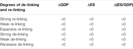
TABLE 1. Degrees of de-linking and re-linking environmental stress (ES).

The decoupling indicator based on the IPAT Equation will be introduced in detail in Section 3.3. Here, some examples using this method are presented along with its advantages and disadvantages. It is not common to find studies that have adopted this method as it is slightly difficult to calculate and cannot distinguish between types of non-decoupling. However, it can be easily applied to relevant planning index calculations. For example, Wang et al. (2013a) examined the decoupling conditions of the domestic extraction of materials, energy use, and sulfur dioxide (SO₂) emissions from the gross domestic product (GDP) of four countries. Lu et al. (2015) analyzed the decoupling of an environmental mountain with case studies from China.

A decomposition analysis used to assess the progress in decoupling industrial growth from CO₂ emissions in an EU manufacturing sector revealed a new method of evaluating decoupling degrees (Diakoulaki and Mandaraka, 2007). The output effect and the non-output effect can be obtained by decomposition analysis, and the calculation of decoupling index based on the ratio of non-output effect and output effect. Evaluating decoupling degrees with this method is clear. A variety of studies use this method — for example, a decomposition of the decoupling of energy-related CO₂ emissions and economic growth in Jiangsu, China (Wang et al., 2013b) and the decomposition of energy-related carbon emissions and its decoupling from economic growth in China (Zhang and Da, 2015).

To evaluate the degree of decoupling with the method of statistical analysis, we should establish a functional relationship between energy pressure and GDP using a regression analysis followed by a relative coefficient that includes the Tapio method to obtain the result. There are some advantages of this method. We can ignore any unnecessary factors and focus on the key factors. it can evaluate the degree of decoupling and quantitatively analyze the driving factors — for example, the decoupling of industrial energy consumption and CO₂ emissions in energy intensive industries in Scandinavia (Enevoldsen et al., 2007), and the decoupling relationship between biophysical and socioeconomic variables and runoff and sediment yield in public catchments of Jiangxi province (Yu et al., 2021).

In the above method, the Tapio method fractionizes the decoupling stated, making it more accurate than the OECD method. Compared with the Tapio method, the statistical analysis method shows higher precision. However, it requires a pretty large amount of data. There is the same problem with the index decomposition method. The Vehmas method is simple and obvious but the critical state of the degrees was not considered, nor can it contribute to the evaluation of a long-term plan. Contrasting to other methods, the IPTA model is more easily to apply to the calculation of relevant planning indicators.

As shown in Table 2, we can identify the characteristics of these six methods. This paper attempts to apply the decoupling index presented by Tapio and the IPAT model to examine the occurrence of non-synchronous variations between GDP and the water footprint in Beijing from 1980 to 2013 and compare the results derived from these two methods.

TABLE 2

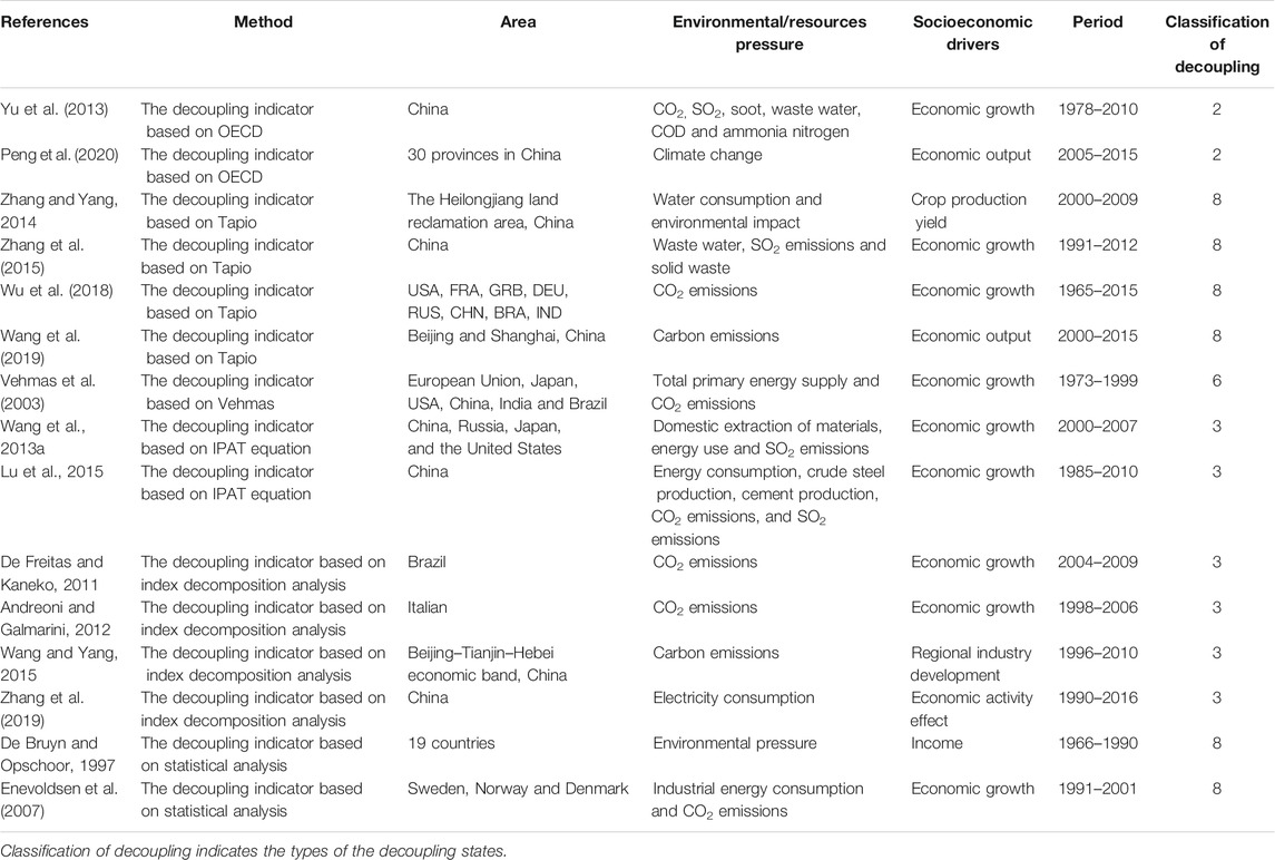
TABLE 2. Comparison of different methods for measuring decoupling.

3 Methods and Data

3.1 WF Evaluation

The water footprint (WF) of crop production is calculated using the following formulas (Hoekstra et al., 2011).

$WF=W{F}_{blue}+W{F}_{green}+W{F}_{grey}(1)$

$W{F}_{blue}=\frac{CW{U}_{blue}}{Y}\times C=10\times \frac{E{T}_{blue}}{Y}\times C(2)$

$W{F}_{green}=\frac{CW{U}_{green}}{Y}\times C=10\times \frac{E{T}_{green}}{Y}\times C(3)$

$W{F}_{grey}=\frac{\left(\alpha \times AR\right)/\left(C_{\max }-C_{nat}\right)}{Y}\times C(4)$

where WF is the water footprint of the crop (m³), CWU_blue is the blue water in crop water consumption (m³ha⁻¹), CWU_green is the green water in crop water consumption (m³ha⁻¹), 10 is the factor that converts the water depth (mm) into water volume per area (m³ha⁻¹) (Hoekstra et al., 2011), ET_blue is the blue water evapotranspiration (mm), ET_green is the green water evapotranspiration (mm), Y is the crop yield per unit area (kg ha⁻¹) (Hoekstra et al., 2011), C is the crop yield (t), AR is the amount of fertilizer used per unit area (kg hm⁻²), α is the leaching rate (the proportion of pollutants into the water out of all the fertilizer), C_max is the maximum allowable concentration (kg m⁻³), and C_nat is the natural background concentration (kg m⁻³).

3.2 Decoupling Indicator Based on Tapio

Based on the calculation formula used in evaluating the CO₂ emission-economic growth linkage (Tapio, 2005), we can examine the occurrence of decoupling between the growth rates in economic activity and the crop product water footprint from energy consumption in the calculation framework as follows.

$T=\frac{\%\Delta WF}{\%\Delta GDP}=\frac{\%\left(WF-W{F}^{\text{'}}\right)/W{F}^{\text{'}}}{\%\left(GDP-GD{P}^{\text{'}}\right)/GD{P}^{\text{'}}}(5)$

where T is the decoupling index; WF and WF^’ are the water footprint from the target year and base year (m³), respectively; GDP and GDP^’ are the agricultural GDP from the target year and base year (yuan), respectively.

The decoupling state takes the following eight cases:

(1) If 0 < T ≤ 0.8, %ΔWF >0, %ΔGDP> 0, weak decoupling is indicated.

(2) If 0.8 < T ≤ 1.2, %ΔWF >0, %ΔGDP> 0, expansive coupling is indicated.

(3) If T > 1.2, %ΔWF >0, %ΔGDP> 0, expansive negative decoupling is indicated.

(4) If T ≤ 0, %ΔWF <0, %ΔGDP> 0, strong decoupling is indicated.

(5) If T ≤ 0, %ΔWF >0, %ΔGDP< 0, strong negative decoupling is indicated.

(6) If 0 < T ≤ 0.8, %ΔWF <0, %ΔGDP<0, weak negative decoupling is indicated.

(7) If 0.8 < T ≤ 1.2, %ΔWF <0, %ΔGDP<0, recessive coupling is indicated.

(8) If T > 1.2, %ΔWF <0, %ΔGDP<0, recessive decoupling is indicated.

3.3 Decoupling Indicator Based on an IPAT Equation

The decoupling indicator of IGT is derived from a famous IPAT Equation (Commoner, 1972; Ehrlich and Holdren, 1972):

$I=P\times A\times T(6)$

where I is environmental impact, P is the population, A is the per capita GDP, and T is technology (impacts/unit of GDP).

$G=P\times A(7)$

Substituting Eq. 7 into Eq. 6, we can obtain the following IGT Equation (Lu and Mao, 2003; Lu, 2005, 2007, 2008, 2009):

$I=G\times T(8)$

where G is the GDP, which we regard as agricultural GDP; I is redefined as resource use, which we regard as the water footprint; and T is resource use per unit of agricultural GDP.

To evaluate the decoupling between agricultural GDP and the water footprint, Eq. 8 is deduced from the following Equation (Lu et al., 2011),

$I_0=G_0\times T_0(9)$

where G₀ is the agricultural GDP in the base year, I₀ is the water footprint in the base year, and T₀ is the resource use per unit of agricultural GDP in the base year.

We define g as the agricultural GDP growth rate (which is positive when the agricultural GDP growth rate increases and is negative when it decreases) and t as the decreasing rate of the water footprint per unit of agricultural GDP (which is positive when the water footprint per unit of agricultural GDP decreases and is negative when the water footprint increases).

Thus, we can obtain these Equations as follows (Lu et al., 2011).

$I_n=G_n\times T_n(10)$

$G_n=G_0\times {\left(1+g\right)}^n(11)$

$T_n=T_0\times {\left(1-t\right)}^n(12)$

where G_n is the agricultural GDP in the target year, I_n is the water footprint in the target year, and T_n is the resource use per unit of agricultural GDP in target year.

Substituting Eqs 11, 12 into Eq. 10, we can obtain this useful Equation (Lu et al., 2011):

$I_n=G_0\times T_0\times {\left[\left(1+g\right)\times \left(1-t\right)\right]}^n(13)$

When n = 1, Eq. 13 can be written as follows (Lu et al., 2011):

$I_1=G_0\times T_0\times \left(1+g\right)\times \left(1-t\right)(14)$

We define k_r as the increasing rate of the water footprint, thus (Lu et al., 2011),

$k_r=\frac{I_1-I_0}{I_0}(15)$

Substituting Eqs 9, 14 into Eq. 15, we can obtain another Equation (Lu et al., 2011):

$k_r=\left(1+g\right)\times \left(1-t\right)-1(16)$

When the water footprint remains constant, a critical condition has been derived — that is (Lu and Mao, 2003; Lu, 2007, 2005, 2008, 2009),

$t_k=\frac{g}{1+g}(17)$

where t_k is the critical value of t and g is the agricultural GDP growth rate.

Three possible cases are presented as follows:

If t = t_k, the water footprint will remain constant.

If t < t_k, the water footprint will increase.

If t > t_k, the water footprint will decrease.

Thus, the ratio t/t_k is the key to evaluating the decoupling between the water footprint and agricultural GDP. This ratio was defined as the decoupling indicator for waste emissions by Lu et al. (2011):

$D_r=\frac{t}{t_k}(18)$

where D_r is the decoupling indicator for waste emissions, which we regard as the decoupling indicator for the water footprint.

Substituting Eq. 17 into Eq. 18, we can obtain the final formula of the decoupling indicator for waste emissions (Lu et al., 2011):

$D_r=\frac{t}{g}\times \left(1+g\right)(19)$

The values of D_r in the different decoupling conditions are shown in Table 3.

TABLE 3

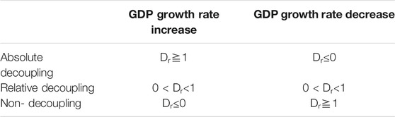
TABLE 3. The values of D_r in the different decoupling conditions.

3.4 Data

When evaluating the water footprint of crop production, we obtained the climate data (1980–2013) in Beijing from the China Meteorological Data Sharing Service System (CMA, 2014), including the relative humidity, hours of sunshine, wind speed, monthly average minimum temperature, monthly average maximum temperature, and precipitation. Agricultural data (1980–2013) were obtained from the Beijing Statistical Yearbook (BBS, 1981-2014), including nitrogen fertilizer data, crop planting area, arable land, and crop production. We also used CROPWAT 8.0 to calculate the crop water requirements and irrigation requirements according to the climate and soil as well as the crop data. Agricultural GDP data were collected from the Beijing Statistical Yearbook (BBS 1981-2014).

4 Results

4.1 Temporal and Spatial Pattern of Crop WF in Beijing

Eight main types of crops were chosen for our study. We calculated their WF from 1980 to 2013 in Beijing. As shown in Figure 1, among the eight main types of crops, the WF of wheat, rice, potatoes, peanuts and maize experienced a gradual downward trend. The WF of wheat and rice fell sharply approximately 2003. The WF of wheat, rice, potatoes, peanuts and maize decreased from 2.17 × 109 m³, 5.54 × 108 m³, 7.63 × 107 m³, 2.14 × 108 m³, and 1.42 × 109 m³ to 3.52 × 108 m³, 2.16 × 106 m³, 8.84 × 106 m³, 2.90 × 10⁷ m³, and 9.35 × 108 m³, respectively. The WF of soybeans and vegetables experienced different trends in different periods from 1980 to 2013, which was a gradual upward trend from 1980 to 2002 followed by a downward period from 2003 to 2013. The WF of soybeans in 2013 is much lower than in 1980, and when compared with soybeans, we can see that the WF of vegetables is very different — 1.6 times greater than the WF from 34 years ago. The WF of melons changed irregularly with the passage of time.

FIGURE 1

FIGURE 1. Changes in the crop WF in Beijing from 1980 to 2013.

Beijing is divided into 16 districts and counties: Dongcheng district, Xicheng district, Chaoyang district, Haidian district, Fengtai district, Shijingshan district, Changping district, Daxing district, Tongzhou district, Shunyi district, Fangshan district, Mentougou district, Huairou district, Pinggu district, Miyun county and Yanqing county. The first six districts is the central municipal district, and the crop yield of them is small. Figure 2 show the spatial pattern of crop WF in Beijing. The agriculture Census Yearbook is the only public source that can directly provide detailed districts and counties agricultural data. However, only two agricultural censuses in Beijing were carried out in 1996 and 2006, respectively. This study depicted the spatial pattern of crop WF in Beijing in 1996 and 2006.

FIGURE 2

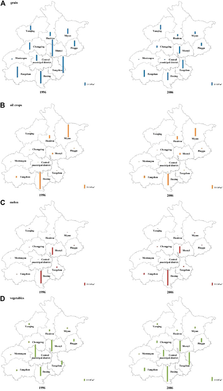
FIGURE 2. The crop WF for districts and counties in Beijing in 1996 and 2006. Panel 2A–D show the spatial pattern of grain WF, oil crops WF, melon WF and vegetables WF respectively.

As shown in Figure 2, comparing 1996 and 2006, the WF of grains in each district and county decreased to different degrees. For other crops, the overall trend was WF decrease in the central municipal district and increase in other districts. The total crop WF in central municipal district in 2006 was reduced by 80.71% compared to the WF in 1996, which is attributed to the municipal development planning of Beijing.

4.2 Decoupling Indicator Based on Tapio

The decoupling state during the 1981 to 2013 period is presented in Figure 3. The WF presented expansive negative decoupling with agricultural GDP growth in 1991, 1992, 1996, 2004, 2005 and 2006. Among these, the decoupling indexes in 2004, 2005 and 2006 were 3.19, 9.01 and 33.63, respectively. The development in 1986, 2008, 2009 and 2011 presented expansive coupling. Weak decoupling appeared in 1983, 1988, 1994 and 1995. However, strong decoupling occurred in the other years of the study period. Six decoupling indexes stand out, which is the period from 1998 to 2003. The decoupling indexes were −9.34, −2.85, −18.54, −9.21, −5.76 and −11.24, respectively. As a whole, during the 33-years study period, 6 years presented expansive negative decoupling, 4 years presented expansive coupling, 4 years presented weak decoupling and 19 years presented strong decoupling.

FIGURE 3

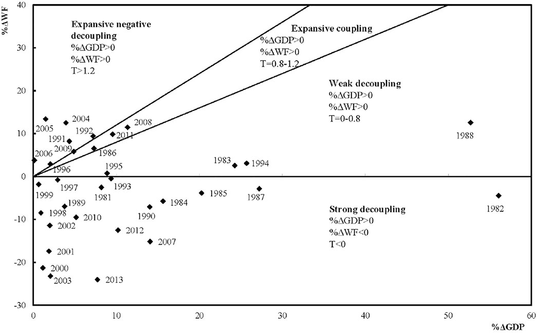
FIGURE 3. The degrees of coupling and decoupling of WF growth from agricultural GDP growth (based on Tapio).

4.3 Decoupling Indicator Based on the IPAT Equation

When we use the method based on the IPAT Equation, we can obtain the decoupling degree for every year, which are shown in Figure 4. This figure vividly describes the decoupling states, in which the agricultural GDP growth rate (g) is on the x-axis, the decoupling indicator for resource use (D_r) is on the y-axis, and t is on each curve. When D_r is positive, it is above the origin or below the origin.

FIGURE 4

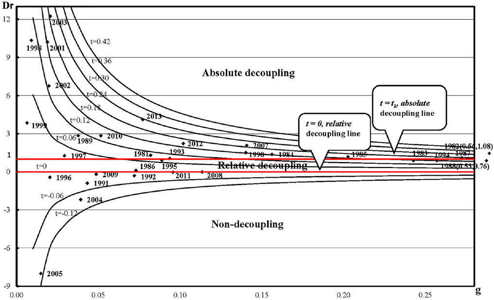
FIGURE 4. The degrees of coupling and decoupling of WF growth from agricultural GDP growth (based on the IPAT equation).

Two lines in the chart are particularly important. One is line t = 0, which means that the resource use increases or decreases contemporaneously with agricultural GDP. The other line is D_r = 1, which means that the resource use remains constant, regardless of how agricultural GDP changed.

As shown in Figure 4, a similar conclusion can be drawn as in Section 4.2. The WF presented non-decoupling with agricultural GDP growth in 1991, 1992, 1996, 2004, 2005, 2006, 2008, 2009 and 2011. Among these years, the decoupling indexes (D_r) in 2004, 2005 and 2006 were -2.19, -8.01 and -32.63, respectively. The decoupling indexes (D_r) in 2008, 2009 and 2011 were -0.01, -0.20 and -0.03, respectively, which are close to relative decoupling. Relative decoupling appeared in 1983, 1986, 1988, 1994 and 1995. However, absolute decoupling occurred in the other years during the study period. As in Section 4.2, the period from 1998 to 2003 was unique. The decoupling indexes (D_r) for this period were huge, which means a high degree of absolute decoupling. To summarize, during the 33-years study period, 9 years presented non-decoupling, 5 years presented relative decoupling and 19 years presented absolute decoupling. Thus, more than seventy percent of the years in the study period presented decoupling. In Figure 4, for the majority of the points, four points (in 1982, 1988, 2000 and 2006) are outside of the figure area.

5 Discussion

As shown in Figures 3, 4, we can obtain similar outcomes. However, we can see that the outcome is described in more detail when based on Tapio. Consequently, we analyze the result based on Tapio to obtain a better evaluation of the decoupling degrees of WF growth from agricultural GDP growth. As vividly depicted in Figure 3, during the study period, the decoupling state changed significantly and experienced different trends in different periods from 1981 to 2013. According to the decoupling states, the entire study period is divided into three periods. We define 1981–1992 as Period I, 1993–2003 as Period II and 2004–2013 as Period III.

Although the decoupling states represent seventy-five percent of Period I, the decoupling degree of this period is not strong. Since China launched its open-door policy and economic reform program in the later part of 1978, the government has attached great importance to the development of agriculture. From 1982 to 1986, the Central Committee of the Chinese Communist Party successively released five “No. 1” documents (the No.1 document originally denoted the first document released by the Central Committee of Chinese Communist Party each year; the No. 1 document now is defined as an issue that is significant for issues related to agriculture, the countryside and the rural population). Beijing, the capital of China, actively responded to the national call. Agriculture was suitably prioritized in the national economy, and the agricultural market demand was expanded. Due to these policies that proceeded from the realities of rural life and the respect shown for the wishes of the rural population, the enthusiasm of this population improved. All in all, the agricultural GDP was not only stable but continued to growing. However, because of the lag in agricultural technology, the problem of the low efficiency of irrigation water was extremely serious. The WF experienced a gradual upward trend in Period I (Xu et al., 2015). To some extent, agricultural development relied on water.

Period 1993–2003 is defined as Period II. More than ninety percent of the WF presented a strong decoupling with agricultural GDP growth in these years. From the decoupling indexes, we can see the degree of decoupling is strong. During Period II, Beijing seriously lacked water resources; therefore, the development of water-saving agricultural practices was of great importance. From 1995 to 2000, $4\times {10}^{4}h{m}^2$ new fields were equipped with water-saving irrigating systems. The area of fields that were irrigated with reclaimed water was $1.47\times {10}^{4}h{m}^2$, and the amount of farmland that was equipped with water-saving irrigating systems totaled $26.67\times {10}^{4}h{m}^2$ (BWCB, 2000). At the same time, with the application of pest control and the mechanization of farming, agricultural productivity and land use efficiency improved greatly. Because the government was vigilant to constantly improve agricultural productivity and strengthen the contribution made by the technological effect of saving water, a harmonious relationship between the WF and agricultural GDP was created.

Finally, the trend in Period III changed from expansive negative decoupling to strong decoupling. As time passed, new difficulties in agricultural development arose. The development imbalance between the urban and rural areas was serious. The decelerating growth of the agricultural GDP led to expansive negative decoupling from 2004 to 2006. In the face of this difficult situation, the Central Committee of the Chinese Communist Party released a new “No. 1” document every year beginning in 2004. The main idea of these documents was to increase the farmers’ income, improve agricultural productivity and develop modern agricultural practices. As a result, agricultural GDP increased rapidly. Furthermore, the government optimized the water-saving irrigation system. Significant progress was made in the water efficiency of irrigation. According to the statistics, the water efficiency of irrigation in Beijing increased from 0.675 in 2007 (BWA, 2008) to 0.69 in 2013 (BWA, 2014). We can see that the WF experienced a downward trend in the latter part of Period III. From 2007 to 2013, although the WF decreased from $2.3\times {10}^9{m}^3$ to $1.8\times {10}^9{m}^3$, the agricultural GDP increased from $1.0\times {10}^{10}RMB$ to $1.6\times {10}^{10}RMB$. Moreover, the decoupling indexes changed from −1.1 to −3.1, and the degree of decoupling became much stronger. Along with the implementation of the Strictest Administration of Water Resources in Beijing, which was issued by the State Council of China in 2012, the government emphasized the importance of high efficiency water saving practices (Fana et al., 2015). With the improvement of the water-saving system, water consumption was successfully controlled. The result suggested that harmonious and sustainable development between WF and agricultural GDP can be realized with effort.

Beijing is experiencing a serious lack of water, which is certainly a main factor in the restriction of the development of the social economy. To ease the local water pressure, Beijing is accelerating progress on the South-to-North Water Transfer Project. It is said that Beijing will benefit from the important strategic project and import 12,000 million tons of fresh water annually by 2020 (Kim, 2003), which will greatly support and ease pressure on the local water supply. Although large amounts of freshwater will be imported, this program cannot promote the degree of decoupling between WF and agricultural GDP. Thus, we should take some other action to improve the situation.

Irrigation water consumption is directly affected by structural changes in agricultural production. It is advisable to adjust plantation structures and plant crops with high yields and lower water demands. Water-intensive crops such as rice are not recommended for planting in Beijing. Thus, large quantities of crop products are imported from geographically adjacent provinces like Hebei, Shandong, and Henan (Xu et al., 2015). Beijing no longer grows rice as a main staple food but instead relies entirely on imports (Huang et al., 2012).

Furthermore, since the water-saving technology achieved remarkable success during Period II and Period III, we must continue to develop water-saving techniques and use more modern facilities in the course of agricultural modernization. Therefore, the original agricultural infrastructure will be replaced by a better infrastructure. For instance, compared with traditional irrigation methods, drip irrigation technology can reduce labor intensity as well as increase crop production. In addition, to some extent, destruction of the environment by human activities cannot be neglected. We must implement more policies that serve to improve awareness of the importance of saving water, such as the Strictest Administration of Water Resources in Beijing, which was issued by the State Council of China in 2012 (Fana et al., 2015).

The occurrence of non-synchronous changes between agricultural GDP and crop WF can be investigated by structural indicators, which play an important role in promoting sustainable water use. However, some other socioeconomic drivers have not been considered yet. For instance, population, urbanization level and technical level may have a significant impact on environmental/resources pressure (Wei et al., 2017). The relationship between these socioeconomic drivers and crop WF is complex, which is worth further investigating.

6 Conclusion

This study evaluated the WF of eight main types of crops in Beijing from 1980 to 2013 and serves as a preliminary attempt to apply the decoupling theory to examine the occurrence of decoupling between agricultural GDP and the crop water footprint. For Beijing, the WF of crop production in 2013 was reduced by 62.1% compared to the WF in 1980; this totals 1.81 × 109 m³. The WF of wheat, rice, potatoes, peanuts and maize experienced a gradual downward trend. The WF of soybeans and vegetables experienced a gradual upward trend from 1980 to 2002 and then saw a downward trend from 2003 to 2013. The WF of soybeans in 2013 was much lower than in 1980, while the WF of vegetables is 1.6 times greater than the WF from 34 years ago.

Furthermore, this study obtained similar outcomes by using two different decoupling indicators. From 1981 to 2013, the decoupling states represented seventy-five percent of the years between 1981 and 1992 (Period I) with a moderate decoupling degree, more than ninety percent from 1993 to 2003 (Period II) with a very strong decoupling degree and experienced a shift from non-decoupling to strong decoupling from 2004 to 2013 (Period III). Overall, more than seventy percent of the years in the study period presented decoupling. As a water-deficient region, adjusting the plantation structure, improving water-saving technology, using more modern facilities and launching more policies to raise awareness of the importance of saving water can promote the degree of decoupling between WF and agricultural GDP.

Data Availability Statement

The original contributions presented in the study are included in the article/Supplementary Material, further inquiries can be directed to the corresponding authors.

Author Contributions

KH: Supervision, Investigation, Funding acquisition; MW: Investigation, Writing-Original draft preparation; ZZ: Supervision, Writing-Reviewing and Editing; YY: Writing-Reviewing and Editing; YB: Data curation.

Funding

This research was supported by the Beijing Natural Science Foundation (9172012) and National Natural Science Foundation of China (52070017).

Conflict of Interest

The authors declare that the research was conducted in the absence of any commercial or financial relationships that could be construed as a potential conflict of interest.

Publisher’s Note

All claims expressed in this article are solely those of the authors and do not necessarily represent those of their affiliated organizations, or those of the publisher, the editors, and the reviewers. Any product that may be evaluated in this article, or claim that may be made by its manufacturer, is not guaranteed or endorsed by the publisher.

Reference

Allan, J. A. (1993). Fortunately There Are Substitutes for Water: Otherwise Our Hydropolitical Futures Would Be Impossible. London, United Kingdom: Overseas Development Administration.

Google Scholar

Andreoni, V., and Galmarini, S. (2012). Decoupling Economic Growth from Carbondioxide Emissions: A Decomposition Analysis of Italian Energy Consumption. Energy. 44(1), 682-691.

CrossRef Full Text | Google Scholar

BBS (1981-2014). Beijing Statistics Yearbook. Beijing, China: China Statistics Press. In Chinese.

Google Scholar

BWA (2008). The Calculation and Analysis Results of Effective Utilization Coefficient of Irrigated Water in Beijing 2007. Beijing: China Water and Hydropower Publisher

Google Scholar

BWA (2014). The Calculation and Analysis Results of Effective Utilization Coefficient of Irrigated Water in Beijing 2013. Beijing: China Water and Hydropower Publisher

Google Scholar

BWCB (2000). Sustainable Utilization Planning of Beijing Water Resources of Initial Decades in the 21st century. Beijing: China Water and Hydropower Publisher, 1–30.

Google Scholar

Cao, X., Xiao, J., Wu, M., Zeng, W., and Huang, X. (2021). Agricultural Water Use Efficiency and Driving Force Assessment to Improve Regional Productivity and Effectiveness. Water Resour. Manage. 35 (8), 2519–2535. doi:10.1007/s11269-021-02845-z

CrossRef Full Text | Google Scholar

Chapagain, A. K., and Hoekstra, A. Y. (2011). The Blue, green and Grey Water Footprint of rice from Production and Consumption Perspectives. Ecol. Econ. 70 (4), 749–758. doi:10.1016/j.ecolecon.2010.11.012

CrossRef Full Text | Google Scholar

CMA (2014). China Meteorological Data Sharing Service System. Beijing. Available at: http://cdc.cma.gov.cn/

Google Scholar

Commoner, B. (1972). “The Environmental Cost of Economic Growth,” in Population, Resources and the Environment. Editor R. G. Ridker (Washington, DC: U.S: Government Printing Office), 339–363.

Google Scholar

Deng, J., Li, C., Wang, L., Yu, S., Zhang, X., and Wang, Z. (2021). The Impact of Water Scarcity on Chinese Inter-provincial Virtual Water Trade. Sustain. Prod. Consumption 28, 1699–1707. doi:10.1016/j.spc.2021.09.006

CrossRef Full Text | Google Scholar

De Bruyn, S. M., and Opschoor, J. B. (1997). Developments in the Throughput-Income Relationship: Theoretical and Empirical Observations. Ecol. Econ. 20(3), 255-268.

CrossRef Full Text | Google Scholar

De Freitas, L. C., and Kaneko, S. (2011). Decomposing the Decoupling of CO₂ Emissions and Economic Growth in Brazil. Ecol. Econ. 70(8), 1459-1469.

CrossRef Full Text | Google Scholar

Diakoulaki, D., and Mandaraka, M. (2007). Decomposition Analysis for Assessing the Progress in Decoupling Industrial Growth from CO2 Emissions in the EU Manufacturing Sector. Energ. Econ. 29 (4), 636–664. doi:10.1016/j.eneco.2007.01.005

CrossRef Full Text | Google Scholar

Ehrlich, P. R., and Holdren, J. P. (1972). Critique. Bull. At. Scientists 28 (5), 16–27. doi:10.1080/00963402.1972.11457930

CrossRef Full Text | Google Scholar

Enevoldsen, M. K., Ryelund, A. V., and Andersen, M. S. (2007). Decoupling of Industrial Energy Consumption and CO2-emissions in Energy-Intensive Industries in Scandinavia. Energ. Econ. 29 (4), 665–692. doi:10.1016/j.eneco.2007.01.016

CrossRef Full Text | Google Scholar

Fan, L., Wang, H., Lai, W., and Wang, C. (2015). Administration of Water Resources in Beijing: Problems and Countermeasures. Water Policy 17 (4), 563–580. doi:10.2166/wp.2014.407

CrossRef Full Text | Google Scholar

Hoekstra, A. Y., Chapagain, A. K., Aldaya, M. M., and Mekonnen, M. M. (2011). The Water Footprint Assessment Manual: Setting the Global Standard. London: UK: Earthscan.

Google Scholar

Huang, J., Zhang, H.-L., Tong, W.-J., and Chen, F. (2012). The Impact of Local Crops Consumption on the Water Resources in Beijing. J. Clean. Prod. 21 (1), 45–50. doi:10.1016/j.jclepro.2011.09.014

CrossRef Full Text | Google Scholar

Huang, K., Wang, Z., Yu, Y., and Yang, S. (2015). Assessing the Environmental Impact of the Water Footprint in Beijing, China. Water Policy 17 (5), 777–790. doi:10.2166/wp.2015.085

CrossRef Full Text | Google Scholar

Hubacek, K., Guan, D., Barrett, J., and Wiedmann, T. (2009). Environmental Implications of Urbanization and Lifestyle Change in China: Ecological and Water Footprints. J. Clean. Prod. 17 (14), 1241–1248. doi:10.1016/j.jclepro.2009.03.011

CrossRef Full Text | Google Scholar

Kim, H. S. (2003). Sustainable Development and the South-To-North Water Transfer Project in China. New Britain, Connecticut: Central Connecticut State University.

Google Scholar

Li, C., Hu, H., Deng, L., Liu, Y., and Wang, Z. (2021). Structural Decoupling the Sectoral Growth from Complete Energy Consumption in China. Energ. Strategy Rev. 34, 100634. doi:10.1016/j.esr.2021.100634

CrossRef Full Text | Google Scholar

Lu, Z. W. (2008). Crossing "environmental Mountain"-Study of Industrial Ecology. Beijing, China: Science Press.

Google Scholar

Lu, Z. W., and Mao, J. S. (2003). Crossing "environmental Mountain"-On the Increase and Decrease of Environment Load in the Process of Economic Growth. Eng. Sci. 5 (12), 36–42.

Google Scholar

Lu, Z. W. (2005). Striving for Better Environmental Protection Plan by Controlling Resource Use as its Breach. Res. Environ. Sci. 18 (6), 1–6. doi:10.13198/j.res.2005.06.3.luzhw.001

CrossRef Full Text | Google Scholar

Lu, Z. W. (2009). The Foundations of Industrial Ecology. Beijing,China: Science Press.

Google Scholar

Lu, Z. W. (2007). The Quantitative Relationship between Economic Growth and Environmental Load. Envrionmental Prot. (7), 13–18. doi:10.1080/14697680600895039

CrossRef Full Text | Google Scholar

Lu, Z., Wang, H., and Yue, Q. (2015). Decoupling Analysis of the Environmental Mountain—with Case Studies from China. J. Ind. Ecol. 19(6), 1082-1090.

CrossRef Full Text | Google Scholar

Lu, Z. W., Wang, H. M., and Yue, Q. (2011). Decoupling Indicators: Quantitative Relationships between Resource Use, Waste Emission and Economic Growth. Resour. Sci. 33 (01), 2–9.

Google Scholar

OECD (2002). Indicators to Measure Decoupling of Environmental Pressure from Economic Growth. SG/SD (2002) 1/Final. Sustainable Development. Available at: http://www.olis.oecd.org/olis/2002doc.nsf/LinkTo/sg-sd(2002)1-final (Accessed 08 28, 10).

Google Scholar

Peng, X., Tao, X., Feng, K., and Hubacek, K. (2020). Drivers toward a Low-Carbon Electricity System in China's Provinces. Environ. Sci. Technol. 54 (9), 5774–5782. doi:10.1021/acs.est.0c00536

PubMed Abstract | CrossRef Full Text | Google Scholar

Song, W., and Liu, M. (2014). Assessment of Decoupling between Rural Settlement Area and Rural Population in China. Land Use Policy 39, 331–341. doi:10.1016/j.landusepol.2014.02.002

CrossRef Full Text | Google Scholar

Tang, Z., Shang, J., Shi, C., Liu, Z., and Bi, K. (2014). Decoupling Indicators of CO2 Emissions from the Tourism Industry in China: 1990-2012. Ecol. Indicators 46, 390–397. doi:10.1016/j.ecolind.2014.06.041

CrossRef Full Text | Google Scholar

Tapio, P. (2005). Towards a Theory of Decoupling: Degrees of Decoupling in the EU and the Case of Road Traffic in Finland between 1970 and 2001. Transport Policy 12 (2), 137–151. doi:10.1016/j.tranpol.2005.01.001

CrossRef Full Text | Google Scholar

Vehmas, J., Kaivo-oja, J., and Luukkanen, J. (2003). Global Trends of Linking Environmental Stress and Economic Growth. Turku: Finland Futures Research Centre, 6–9.

Google Scholar

Wang, H., Hashimoto, S., Yue, Q., Moriguchi, Y., and Lu, Z. (2013a). Decoupling Analysis of Four Selected Countries. J. Ind. Ecol. 17 (4), 618–629. doi:10.1111/jiec.12005

CrossRef Full Text | Google Scholar

Wang, K., Shao, D. G., Gu, W. Q., Cen, D. H., Tan, X. Z., and Yang, F. S. (2011). Decoupling Analysis between Water Consumption and Economic Growth in China. J. Irrigation Drainage 30 (03), 34–38. doi:10.13522/j.cnki.ggps.2011.03.008

CrossRef Full Text | Google Scholar

Wang, Q., Zhao, M., and Li, R. (2019). Decoupling Sectoral Economic Output from Carbon Emissions on City Level: A Comparative Study of Beijing and Shanghai, China. J. Clean. Prod. 209, 126–133. doi:10.1016/j.jclepro.2018.10.188

CrossRef Full Text | Google Scholar

Wang, W., Liu, R., Zhang, M., and Li, H. (2013b). Decomposing the Decoupling of Energy-Related CO2 Emissions and Economic Growth in Jiangsu Province. Energ. Sustain. Develop. 17 (1), 62–71. doi:10.1016/j.esd.2012.11.007

CrossRef Full Text | Google Scholar

Wang, X., Huang, K., Yu, Y., Hu, T., and Xu, Y. (2016). An Input-Output Structural Decomposition Analysis of Changes in Sectoral Water Footprint in China. Ecol. Indicators 69, 26–34. doi:10.1016/j.ecolind.2016.03.029

CrossRef Full Text | Google Scholar

Wang, Z., Huang, K., Yang, S., and Yu, Y. (2013c). An Input-Output Approach to Evaluate the Water Footprint and Virtual Water Trade of Beijing, China. J. Clean. Prod. 42, 172–179. doi:10.1016/j.jclepro.2012.11.007

CrossRef Full Text | Google Scholar

Wang, Z., and Yang, L. (2015). Delinking Indicators on Regional Industry Development and Carbon Emissions: Beijing–Tianjin–Hebei Economic Band Case. Ecol. Indic. 48, 41-48.

CrossRef Full Text | Google Scholar

Wei, J., Huang, K., Yang, S., Li, Y., Hu, T., and Zhang, Y. (2017). Driving Forces Analysis of Energy-Related Carbon Dioxide (CO 2 ) Emissions in Beijing: an Input-Output Structural Decomposition Analysis. J. Clean. Prod. 163, 58–68. doi:10.1016/j.jclepro.2016.05.086

CrossRef Full Text | Google Scholar

Wu, L., Huang, K., Ridoutt, B. G., Yu, Y., and Chen, Y. (2021). A Planetary Boundary-Based Environmental Footprint Family: From Impacts to Boundaries. Sci. Total Environ. 785, 147383. doi:10.1016/j.scitotenv.2021.147383

CrossRef Full Text | Google Scholar

Wu, Y., Zhu, Q., and Zhu, B. (2018). Decoupling Analysis of World Economic Growth and CO2 Emissions: A Study Comparing Developed and Developing Countries. J. Clean. Prod. 190, 94–103. doi:10.1016/j.jclepro.2018.04.139

CrossRef Full Text | Google Scholar

Xu, Y., Huang, K., Yu, Y., and Wang, X. (2015). Changes in Water Footprint of Crop Production in Beijing from 1978 to 2012: a Logarithmic Mean Divisia index Decomposition Analysis. J. Clean. Prod. 87, 180–187. doi:10.1016/j.jclepro.2014.08.103

CrossRef Full Text | Google Scholar

Yu, S., Xie, C., Zhao, J., Zhen, W., Ling, W., and Shi, Z. (2021). Socioeconomic Development Mitigates Runoff and Sediment Yields in a Subtropical Agricultural Watershed in Southern China. Environ. Res. Lett. 16 (2), 024053. doi:10.1088/1748-9326/abdd5a

CrossRef Full Text | Google Scholar

Yu, Y., Chen, D., Zhu, B., and Hu, S. (2013). Eco-efficiency Trends in China, 1978-2010: Decoupling Environmental Pressure from Economic Growth. Ecol. Indicators 24, 177–184. doi:10.1016/j.ecolind.2012.06.007

CrossRef Full Text | Google Scholar

Zhang, C., Su, B., Zhou, K., and Yang, S. (2019). Analysis of Electricity Consumption in China (1990-2016) Using index Decomposition and Decoupling Approach. J. Clean. Prod. 209, 224–235. doi:10.1016/j.jclepro.2018.10.246

CrossRef Full Text | Google Scholar

Zhang, Y.-J., and Da, Y.-B. (2015). The Decomposition of Energy-Related Carbon Emission and its Decoupling with Economic Growth in China. Renew. Sustain. Energ. Rev. 41, 1255–1266. doi:10.1016/j.rser.2014.09.021

CrossRef Full Text | Google Scholar

Zhang, Y., Huang, K., Yu, Y., and Yang, B. (2017). Mapping of Water Footprint Research: A Bibliometric Analysis during 2006-2015. J. Clean. Prod. 149, 70–79. doi:10.1016/j.jclepro.2017.02.067

CrossRef Full Text | Google Scholar

Zhang, Z., Chen, X., Heck, P., Xue, B., and Liu, Y. (2015). Empirical Study on the Environmental Pressure versus Economic Growth in China during 1991-2012. Resour. Conserv. Recycling 101, 182–193. doi:10.1016/j.resconrec.2015.05.018

CrossRef Full Text | Google Scholar

Zhang, Z. (2000). Decoupling China's Carbon Emissions Increase from Economic Growth: An Economic Analysis and Policy Implications. World Develop. 28 (4), 739–752. doi:10.1016/s0305-750x(99)00154-0

CrossRef Full Text | Google Scholar

Zhang, Y., and Yang, Q. (2014). Decoupling Agricultural Water Consumption and Environmental Impact from Crop Production Based on the Water Footprint Method: A Case Study for the Heilongjiang Land Reclamation Area, China. Ecol. Indic. 43, 29–35.

Google Scholar