 Hamid Salehi
 Ali Shamsoddini2
 Behnam Mirgol
 Meisam Nazari
- 1Department of Water Engineering, Tarbiat Modares University, Tehran, Iran
- 2Department of Remote Sensing and GIS, Tarbiat Modares University, Tehran, Iran
- 3Center for Agroecology, Water and Resilience, Coventry University, Coventry, United Kingdom
- 4Division of Biogeochemistry of Agroecosystems, Georg-August University of Göttingen, Göttingen, Germany
Producing daily actual evapotranspiration (ETa) maps with high spatial resolution has always been a challenge for remote sensing research. This study assessed the feasibility of producing daily ETa maps with a high spatial resolution (30 m) for the sugarcane farmlands of Amir Kabir Sugarcane Agro-industry (Khuzestan, Iran) using three different scenarios. In the first scenario, the reflectance bands of Landsat 8 were predicted from the moderate resolution imaging spectroradiometer (MODIS) imagery using the spatial and temporal adaptive reflectance fusion model (STARFM) algorithm. Also, the thermal bands of Landsat 8 were predicted by the spatiotemporal adaptive data fusion algorithm for temperature mapping (SADFAT). Then, ETa amounts were calculated employing such bands and the surface energy balance algorithm for land (SEBAL). In the second scenario, the input data needed by SEBAL were downscaled using the MODIS images and different methods. Then, using the downscaled data and SEBAL, daily ETa amounts with a spatial resolution of 30 m were calculated. In the third scenario, ETa data acquired by MODIS were downscaled to the scale of Landsat 8. In the second and third scenarios, downscaling of the data was carried out by the ratio, regression, and neural networks methods with two different approaches. In the first approach, the Landsat image on day 1 and the relationship between the two MODIS images on day 1 and the other days were used. In the second approach, the simulated image on the previous day and the relationship between the two consecutive images of MODIS were used. Comparing the simulated ETa amounts with the ETa amounts derived from Landsat 8, the first scenario had the best result with an RMSE (root mean square error) of 0.68 mm day−1. The neural networks method used in the third scenario with the second approach had the worst result with an RMSE of 2.25 mm day−1, which was however a better result than the ETa amounts derived from MODIS with an RMSE of 3.19 mm day−1. The method developed in this study offers an efficient and inexpensive way to produce daily ETa maps with a high spatial resolution. Furthermore, we suggest that STARFM and SADFAT algorithms have acceptable accuracies in the simulation of reflectance and thermal bands of Landsat 8 images for homogeneous areas.
Introduction
Evapotranspiration (ET) is a major component of global water cycle (Sobrino et al., 2021). Precise estimation of actual evapotranspiration (ETa) on different temporal and spatial scales is necessary for various applications such as natural resources and agricultural management, water resources management, irrigation planning, and soil and crop modeling (Steiner et al., 1991; Nassar et al., 2021). Given the limited number of weather stations and high cost and time required for collecting ground data, using remote sensing techniques can be useful for determining ETa, if a good output accuracy is guaranteed. One of the most common methods for determining ETa using remotely sensed data is the surface energy balance algorithm for land (SEBAL) (Bastiaanssen et al., 2002; Bastiaanssen et al., 2005; Li et al., 2021). Hafeez et al. (2002) compared the results of daily ETa calculated by SEBAL using advanced spaceborne thermal emission and reflection radiometer (ASTER) data with ETo (reference ET calculated by the FAO Penman-Monteith method), ETpan (ET measured at weather stations), and ETc (ET calculated having the crop coefficient Kc = 0.9) and indicated that SEBAL is of a good accuracy. In another study, Chandrapala and Wimalasuriya (2003) compared ETa resulted from SEBAL with ETa measured by a scintillometer and showed that the differences between them in 10-days and monthly periods were 17 and 1%, respectively. These studies concluded that SEBAL is of a good performance in estimating ETa.
A balance is established between spatial, temporal, and spectral resolutions in the designing process of satellites (Emelyanova et al., 2013; Zhu et al., 2018; Bai et al., 2020; Moreno-Martinez et al., 2020). Nevertheless, due to technical limitations, most satellites are not able to collect images with high temporal, spatial, and spectral resolutions simultaneously (Ghassemian, 2009; Bai et al., 2015). Many of satellites images of high spatial resolution have lower temporal resolution compared to those with low to average spatial resolutions (Emelyanova et al., 2013; Zhu et al., 2018; Bai et al., 2020). For example, due to their high spatial resolution, Landsat images are used for many environmental applications i.e., production of ETa maps (Fu et al., 2014; Ping et al., 2018). However, there is a huge limitation in using the Landsat imagery for monitoring dynamic changes over land surfaces due to a 16-days temporal resolution and the probability of cloud cover (Gao et al., 2006; Roy et al., 2008; Ping et al., 2018). On the other hand, the moderate resolution imaging spectroradiometer (MODIS) imagery has a daily temporal resolution, but its low spatial resolution limits its performance in environmental applications (Zhu et al., 2010; Gevaert and García-Haro, 2015; Ping et al., 2018). Thus, it has not so far been possible to monitor important environmental phenomena like ETa with the same sensor and high spatial and temporal resolutions. In order for an accurate spatial and temporal estimation of environmental ETa, image fusion methods are usually employed (Ha et al., 2013; Ping et al., 2018). In the process of image fusion, images acquired from two or more sensors are used as input data, and an output that has more information compared to the input images is derived (Roshan et al., 2015; Malhotra et al., 2021). This process of spatial resolution enhancement of remotely sensed data by fusion of separate data is called downscaling (Atkinson, 2013). For instance, downscaling of MODIS images using Landsat data could create images with a spatial resolution of 30 m and a temporal resolution of 1 day (Ke et al., 2016).
To date, various methods have been used and assessed for downscaling remotely sensed data in order to obtain ETa maps with high temporal and spatial resolutions. The downscaling can be conducted in three levels as downscaling of bands, downscaling of input data required for energy balance algorithms, and downscaling of ETa products. For instance, Gao et al. (2006) introduced an algorithm for combining images acquired from the enhanced thematic mapper plus (ETM+) and MODIS in order to achieve images with better clarity and higher temporal and spatial resolutions. They employed the spatial and temporal adaptive reflectance fusion model (STARFM) for prediction of reflectance bands in ETM+. They also used MODIS images at time 1 (the day on which Landsat images are available) and time 2 (the day on which Landsat images are not available) as well as ETM + images at time 1 to predict reflectance bands of ETM+ (i.e., bands 1, 2, 3, 4, 5, 7) at time 2. They compared the downscaled images with the ETM + images and demonstrated that the results were good.
Given the high accuracy of STARFM, it can be used for simulation of Landsat reflectance bands in order to monitor ETa. However, for achieving ETa maps with high temporal and spatial resolutions, thermal bands are also required. Hong et al. (2013) produced high-resolution daily ETa images using two different approaches. In the first approach, they obtained input data for SEBAL (e.g., surface albedo coefficient, normalized difference vegetation index [NDVI] and land surface temperature [LST]) from MODIS, and then downscaled these data to the spatial resolution of Landsat 7 using the subtraction and regression methods and obtained ETa using the downscaled data. In this approach, they calculated a mean absolute difference (MAD) of 0.55 mm day−1 for the subtraction method and 0.54 mm day−1 for the regression method. In the second approach, they obtained ETa using MODIS images and SEBAL, and then downscaled ETa obtained from MODIS to the spatial resolution of Landsat 7 using the subtraction and regression methods. In this approach, a MAD of 0.53 mm day−1 was calculated for the subtraction method and 0.57 mm day−1 for the regression method. Brindhu et al. (2013) conducted a study in Tamil Nadu and parts of the Thamiraparani River Basin (India) with a total area of 5,665 km2 and downscaled LSTs obtained from MODIS with a spatial resolution of 960 m to the scale of Landsat 7 with a spatial resolution of 60 m using the Nonlinear DisTrad method. They compared the LSTs downscaled using the Nonlinear DisTrad method with the LSTs downscaled using the sharpening thermal (TsHARP) method and the LSTs obtained from Landsat 7. In their study, RMSEs were 0.96° K for the Nonlinear DisTrad method and 1.91º K for the TsHARP method. They also compared the ETa amounts resulted from SEBAL using the LSTs downscaled by the Nonlinear DisTrad method, the LSTs downscaled by the TsHARP method, the LSTs obtained from Landsat 7. Their calculated RMSEs for ETa were 0.16 mm day−1 using the LSTs downscaled by the Nonlinear DisTrad method and 0.55 mm day−1 using the LSTs downscaled by the TSHARP method.
For monitoring ETa, reflectance bands are also required. Weng et al. (2014) modified STARFM in order to take into account the annual temperature cycle (ATC) and developed the spatiotemporal adaptive data fusion algorithm for temperature mapping (SADFAT) for downscaling thermal data. They attained a coefficient of determination (R2) of 0.87 between the downscaled and Landsat thermal data. In another study, Mahour et al. (2017) evaluated the effect of downscaling of LSTs by the Co-Kriging method on the estimation of ETa for a farmland located in Qazvin (Iran). They used two approaches for downscaling. In the first approach, the LSTs obtained from MODIS with a spatial resolution of 1,000 m were downscaled to a spatial resolution of 250 m by the Co-Kriging method. They used the outcome and applied the surface energy balance system (SEBS) algorithm for estimating daily ETa with a spatial resolution of 250 m. In the second approach, they downscaled the ETa data obtained from MODIS with a resolution of 1,000 m using SEBS to a spatial resolution of 250 m using the Co-Kriging method. They used the LSTs obtained from Landsat 8 for accuracy assessment. Their results illustrated that a difference of 2.7º K between the LSTs obtained from Landsat 8 and the downscaled LSTs exists. Further, ETa calculated by SEBS and Landsat 8 was 5.76 mm day−1 and the downscaled ETa was 5.57 mm day−1. The RMSE between the reference ETa and the downscaled ETa was 1.26 mm day−1, and the RMSE between the reference LSTs and the downscaled LSTs was 3.67º K. They concluded that LST has a great impact on the estimation of ETa based on remote sensing data.
So far, there has been no study that uses downscaling techniques in three levels including downscaling of bands, downscaling of input data required for the energy balance algorithms, and downscaling of ETa images to obtain daily ETa images with a spatial resolution of 30 m. Thus, the present study aimed to employ downscaling techniques in three different scenarios for producing daily ETa maps with a spatial resolution of 30 m for the sugarcane farmlands of Amir Kabir Sugarcane Agro-industry, Khuzestan, Iran. In the first scenario, the reflectance and thermal bands of Landsat 8 were predicted using STARFM and SADFAT, respectively. Then, ETa was calculated using these bands and SEBAL. In the second scenario, the input data required for SEBAL were downscaled and then daily ETa with a spatial resolution of 30 m was calculated. In the third scenario, the ETa images obtained from MODIS were downscaled to the scale of Landsat 8. In the second and third scenarios, data downscaling was conducted by using the ratio, regression, and neural networks methods with two different approaches. In the first approach, for simulating the data with a spatial resolution of 30 m and a temporal resolution of 1 day, the Landsat image on day 1 and the relationship between the two MODIS images on day 1 and the other days were used. In the second approach, for simulating the data on the desired day, the simulated image on the previous day and the relationship between the two consecutive images of MODIS were used.
Methods
Study Area and Data Acquisition
The study area is the sugarcane farmlands of Amir Kabir Sugarcane Agro-industry. The company is located in south of Khuzestan province, Iran, at 48° 16′ 49″ E and 31° 2’ 2” N. Amir Kabir Sugarcane Agro-industry is located 45 km from Ahwaz-Khorramshahr Road and bordered with Karun River from the east. The gross area of the abovementioned farmlands is 15,000 ha and the net area is 12,000 ha, which is divided into several 25-ha pieces (Figure 1).
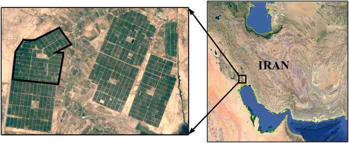
FIGURE 1. Geographical location of the study area.
Satellite data including MODIS images acquired on June 16, 2017 and June 30, 2017 and Landsat 8 images acquired on June 14, 2017, June 30, 2017 and July 16, 2017 were used. The bands used in this study for downscaling including Landsat 8 bands and the corresponding bands in MODIS images are listed in Table 1.
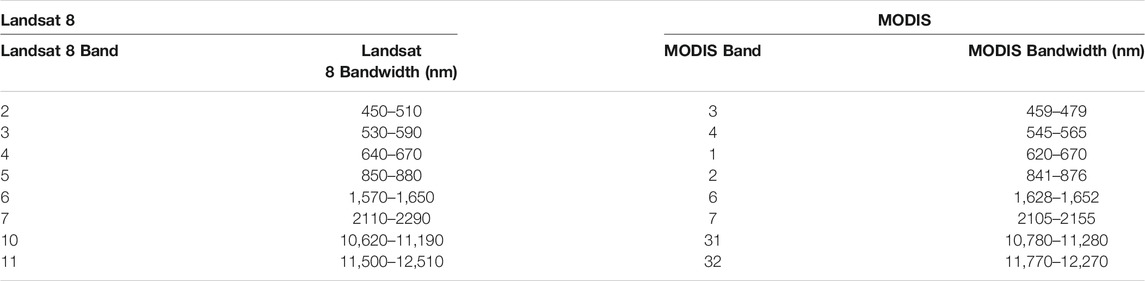
TABLE 1. Bands and bandwidths of Landsat 8 and the corresponding bands and bandwidths in MODIS.
Pre-Processing of Satellite Images
Due to the atmosphere between the sensor and land surface, the reflectance of the surface features before reaching the sensor is affected by two factors of absorption and scattering, leading to uncertainty in determination of the surface reflectance (Kaufman et al., 1997; Gao et al., 2000). In this study, the method introduced by Tasumi et al. (2008) was used for atmospheric correction of the MODIS and Landsat 8 images.
Downscaling of Reflectance Bands Using STARFM
In order to achieve images with high temporal and spatial resolutions, researchers used an image fusion algorithm for combining images of ETM + and MODIS (Gao et al., 2006). This algorithm is abbreviated as STARFM and is a common basic algorithm for temporal and spatial combination of satellite images. It predicts the value of the central pixel in Landsat images at the second time based on the calculation of correct weights for the neighboring pixels. Therefore, this algorithm moves over the Landsat classified image acquired on the first time as a moving window and downscales the image with low spatial resolution acquired at the second time with respect to the images of MODIS acquired at the first and second times and the classified image of Landsat acquired at the first time. The following equation was established for a heterogeneous pixel of MODIS:
where
Equation 1 is logical for homogeneous pixels in MODIS image, but it should be considered that all pixels in MODIS image are not homogeneous and it is possible that the type of land cover changes over the prediction period. Thus, the neighborhood information was used for correcting the surface reflectance by applying a weight function:
where w is the size of the moving window,
For ensuring that the information in Eq. 2 is correct and that the neighboring pixels are homogeneous, only spectrally similar pixels (pixels belonging to one spectral class) were used. A classified Landsat image was needed for achieving this. The ISOData algorithm was used as an unsupervised classification method.
Downscaling of Thermal Bands Using the SADFAT
STARFM has been used for prediction of reflectance bands based on the assumption that surface reflectances in MODIS and Landsat images on the same day are similar (Gao et al., 2006; Masek et al., 2006). For homogeneous pixels, so long as this assumption i.e., band similarity between Landsat and MODIS thermal data on the same day is established, STARFM was used for downscaling thermal images and LST. However, changes of LST over time show that daily and seasonal variations are severe (Sabins, 1997; Weng et al., 2008). Weng et al. (2014) modified STARFM taking into account ATC and heterogeneous urban thermal landscape for prediction of thermal radiance and LST data. They named the new algorithm SADFAT. In this algorithm, the linear spectral mixture analysis (LSMA) was used for relating radiance in the Landsat and MODIS images so that temporal changes in the radiance could be included in the fusion model. For a homogeneous pixel in Landsat image, radiance at tp is equal to the total radiance of Landsat image at t0 and a coefficient of difference in radiance in MODIS images at tp and t0. The required coefficient (a) can be determined through a regression relationship derived from the association between thermal bands of Landsat MODIS images. Since a large number of pixels contain more than one cover type, the radiance of the mixed pixel of the Landsat image was estimated according to the below processes.
The radiance change of the MODIS pixel from t1 to t2 was computed as:
where R is the radiance and M and L are abbreviations of MODIS and Landsat respectively.
Seasonal change in LST was modeled using the annual temperature cycle (ATC) approximated using a sinusoidal function (Bechtel, 2012):
where MAST is the mean annual surface temperature, YAST is the yearly amplitude surface temperature, w is the angular frequency, d is the day of year (DOY) relative to the equinox, and θ is the phase shift. Since spectral radiance is related to LST by the Plank’s law, the radiance change of an L pixel from time t1 to t2 was quantified as:
where θ is the phase shift or heat lag, c is the amplitude of the radiance variation, C is the constant,
If the radiances of the kth L pixel at date t1 and t2 are known, Eq. 4 has an instance as:
By combining Eqs 6, 7, Eq. 8 can be obtained:
Since θ reflects the phase shift of a pixel and is associated with thermal properties of land surface materials, it can be regarded as constant as long as the land cover does not change in the observational period. Therefore, the ratio of the radiance change of kth L pixel to that of the corresponding M pixel is constant for a certain L pixel. Here,
Based on Eq. 8, if one pair of L and M radiance image at t0 and another M radiance image at tp are available, the L radiance image at tp can be predicted using the following formula:
where Wi is the weight of the similar neighboring pixel and N is the number of similar pixels.
The calculated radiance could be converted to LST using Planck’s law. In Eq. 3, the weight of similar neighboring pixels of the central pixel should be calculated. This weight determines the contribution of the neighboring pixels to the calculation of a central pixel. Similarity between reflectance and thermal radiances in a pixel and the central pixel as well as the distance between the central pixel and a neighboring pixel increase the pixel weight.
In the MODIS sensor, thermal bands 31 and 32 are used to estimate LST. For this, the radiance was converted to the brightness temperature using the inverse of the Planck’s law (Lu and Weng, 2006).
where
The constant coefficients
where
In the Landsat 8 satellite, LST is obtained from bands 10 or 11. In this study, LST was obtained from band 10 using Eq. 13.
where
Ratio and Regression Methods
In the ratio and regression methods, for simulation of the Landsat image at T1 (the day on which Landsat images are not available), a relationship was established between the two MODIS images at T0 and T1 by the ratio and regression methods. Then, by assuming that this relationship is also established between the two Landsat images at T0 (the day on which Landsat images are available) and T1 (Hong et al., 2013), the Landsat image at T1 was simulated (Figure 2).
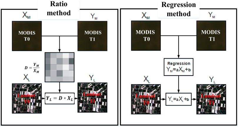
FIGURE 2. Calculation processes based on the ratio and regression methods (Hong et al., 2013).
Neural Networks Method
The neural networks method has different algorithms, one of which is the multi-layer perceptron (MLP). MLP is formed of multiple layers and neurons. It consists of an input layer, one or more hidden layers, and an output layer. One of the differences between different neural networks is their distinct activation functions. In the hidden layer of MLP, mostly three types of sigmoid, hyperbolic and linear (identical) moving functions are used. In the present study, the sigmoid function was used in the hidden layer. Generally, in MLP networks, some factors should be determined properly including the number of hidden layers, the number of neurons in the hidden layers, the learning rate, the momentum, and the error threshold in order to reach a suitable model for solving a specific problem.
SEBAL for Calculation of ETa
The energy balance equation is the basis of remote sensing algorithms for calculation of ETa. The energy balance equation is as follows (Bastiaanssen et al., 1998):
where Rn is net radiation, G is soil heat flux, H is sensible heat flux, λET is latent heat flux, s is biomass energy, P is photosynthesis, and h is the horizontal component of sensible and latent heat fluxes.
In Eq. 4, photosynthesis and heat storage in plants could be ignored, because most plants consume less than 1% of the reached Sun radiation for photosynthesis. Daytime heat storage in plants could also be ignored, because it is important only when temperature changes fast (especially at sunset and sunrise) and when amounts of Rn, H, and λET are small. Moreover, the horizontal component of sensible and latent heat fluxes indicates the net amount of energy exchanged by the plant in a horizontal direction. In dry weather, it can be equal to net radiation, and despite its importance, it is usually not taken into account due to lack of a simple solution for evaluation. Considering such assumptions in the energy balance equation and elimination of those three components, Bastiaanssen et al. (1998) applied an algorithm of land surface energy namely SEBAL using the multi-step physical calculations. The equations and calculation processes for each parameter of Rn, G and H are explained fully in the study of Bastiaanssen et al. (2002). Due to the high efficiency of SEBAL for calculation of ETa, this method was used to evaluate the efficiency of the used scenarios for calculation of daily ETa with a high spatial resolution.
Results
Visual comparison of the simulated bands with the original bands of Landsat 8 (Figure 3) and the RMSE values provided in Table 2 indicated that STARFM had an acceptable performance. Also, comparison of LST determined based on the simulated bands with LST obtained from the original image of Landsat 8 acquired on June 30, 2017 showed that SADFAT was able to simulate the LST distribution well (Figure 4).
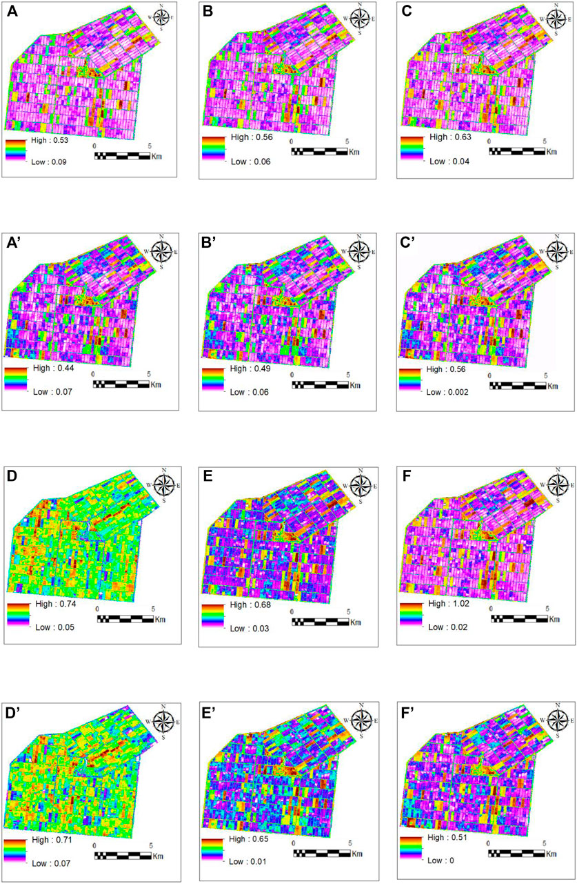
FIGURE 3. Simulated reflectance bands of the sugarcane farmlands of Amir Kabir Sugarcane Agro-industry with the spatial resolution of 30 m using STARFM on June 30, 2017 and the original reflectance bands of the Landsat 8 image on the same day. (A) original band 2, (A׳) simulated band 2, (B) original band 3, (B׳) simulated band 3, (C) original band 4, (C׳) simulated band 4, (D) original band 5, (D׳) simulated band 5, (E) original band 6, (E׳) simulated band 6, (F) original band 7, and (F׳) simulated band 7 on June 30, 2017. White spots on the right edge and central part of the simulated image are cloud cover over these areas.

TABLE 2. Comparison of the simulated and original bands of the Landsat 8 image of the sugarcane farmlands of Amir Kabir Sugarcane Agro-industry on June 30, 2017.
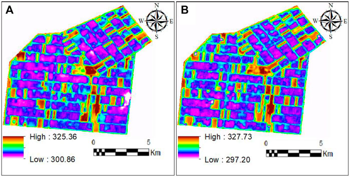
FIGURE 4. Reflectance bands of the land surface temperature (LST) of the sugarcane farmlands of Amir Kabir Sugarcane Agro-industry on June 30, 2017. (A) simulated by SADFAT; (B) obtained from the Landsat 8 image.
In the second scenario, the input data of SEBAL (i.e., surface albedo, NDVI, leaf area index [LAI], and LST) were simulated by the ratio, regression, and neural networks methods with two approaches. In the ratio method, both approaches were the same and had identical performances (Table 3; Figure 5). In the regression method, the R2 values obtained for the input data simulated by the first and the second approaches were the same (Figure 5). ETa obtained by SEBAL for the input data simulated by the regression method with the first and second approaches had the same R2 values but different RMSEs (Table 3; Figure 5). In the neural networks method, the first and second approaches were completely different (Table 3; Figure 5).
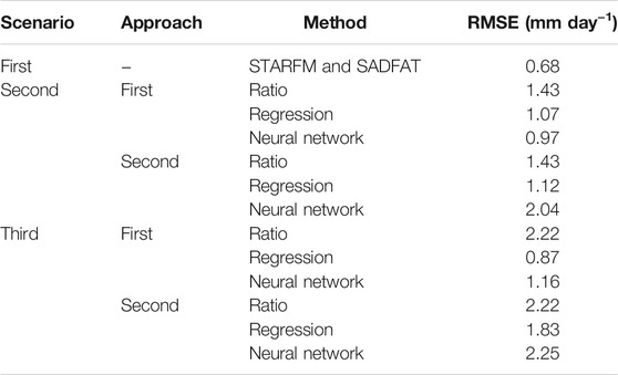
TABLE 3. RMSE values for the simulated ETa amounts.
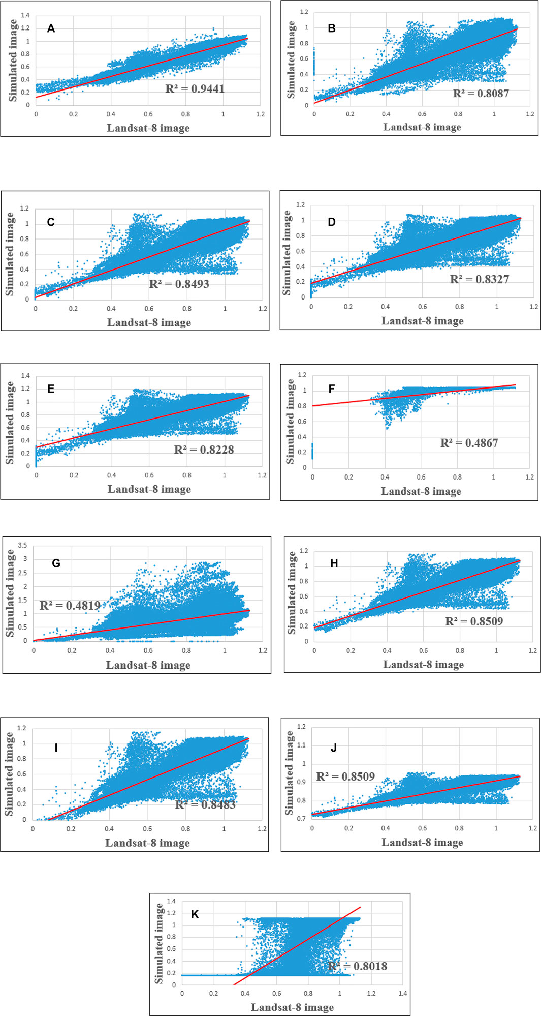
FIGURE 5. Comparison of ETa derived from the simulations and Landsat 8 image: (A) the first scenario, (B) the second scenario, the ratio method (the first and second approaches), (C) the second scenario, the regression method, the first approach, (D) the second scenario, the neural networks method, the first approach, (E) the second scenario, the regression method, the second approach, (F) the second scenario, the neural networks method, the second approach, (G) the third scenario, the ratio method (the first and second scenario), (H) the third scenario, the regression method, the first approach, (I) the third scenario, the neural networks method, the first approach, (J) the third scenario, the regression method, the second approach, (K) the third scenario, the neural networks method, the second approach.
In the third scenario, ETa amounts simulated by the first and second approaches were identical and had equal performances (Table 3; Figure 5). In the regression method, the R2 values calculated for ETa amounts simulated with the first and second approaches were the same, but the RMSEs were different (Table 3; Figure 5). In the neural networks method, the simulated ETa had different R2 values and RMSEs (Table 3; Figure 5).
The simulated ETa images and the ETa images obtained from MODIS and Landsat 8 data on June 30, 2017 were visually compared (Figure 6). In these images, pink points indicate minimum ETa and represent idle lands. Dark brown points show maximum ETa and illustrate lands with dense vegetation. As it is shown in image A2, pixels on the northern and eastern borders of the farmlands had the lower ETa than the other pixels, due to the neighboring barren lands.
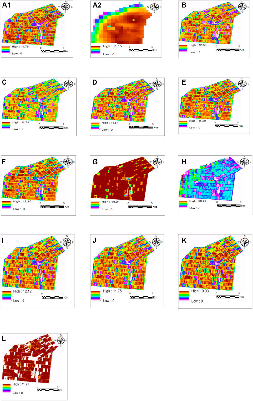
FIGURE 6. Actual evapotranspiration (ETa, mm day−1) images on June 30, 2017 (A1) ETa obtained from Landsat 8 data, (A2) ETa obtained from MODIS data, (B) ETa simulated in the first scenario, (C) ETa simulated in the second scenario by the ratio method (the first and the second approaches), (D) ETa simulated in the second scenario by the regression method with the first approach, (E) ETa simulated in the second scenario by the neural networks method with the first approach, (F) ETa simulated in the second scenario by the regression method with the second approach, (G) ETa simulated in the second scenario by the neural networks method with the second approach, (H) ETa simulated in the third scenario by the ratio method (the first and the second approaches), (I) ETa simulated in the third scenario by the regression method with the first approach, (J) ETa simulated in the third scenario by the neural networks method with the first approach, (K) ET simulated in the third scenario by the regression method with the second scenario, (L) ETa simulated in the third scenario by the neural networks with the second approach.
Discussion
Evaluation of the Used Scenarios
The first scenario with an RMSE of 0.68 mm day−1 had the best performance (Table 3). A major reason for this could be the simulation of the thermal band with higher accuracy in this scenario. In the first scenario, the value of RMSE for the simulated LST on June 30, 2017 is estimated to be 1.95 °K. (Weng et al., 2014) used SADFAT for simulation of LST with the spatial resolution of Landsat 8 and compared the results with the images acquired by Landsat 8. They found RMSE values for the study area to be between 1.32 °K to 2 °K. Their finding is in agreement with the results of the present study. In SADFAT, changes of LST over the time gap between acquisition times of MODIS and Landsat images of the same day are taken into account. Whilst the ratio, regression, and neural networks methods function based on the assumption that LST values obtained from MODIS and Landsat images of the same day are similar. Mahour et al. (2017) also pointed out the importance of thermal data accuracy in determination of ETa.
STARFM was used in the first scenario for simulating the reflectance bands. STARFM had a satisfactory performance in the study area (Table 2). Gao et al. (2006), Hilker et al. (2009), and Bhandari et al. (2012) also reported a high efficiency for STARFM in the simulation of Landsat reflectance bands. STARFM is greatly dependent on the homogeneity of study areas, and heterogeneity and variability of land cover in the area may significantly affect results of this algorithm (Gao et al., 2006). Thus, the homogeneity of the study area in the present study could be the main reason for the high R2 (except band 5) and low RMSE values for the simulated bands. A major reason for the reduced R2 of band 5 can be the existence of uncertainties related to downscaling. Bhandari et al. (2012) found low R2 for bands 1 and 2 but suggested no specific reason for this. Rather than being an accuracy indicator, R2 is a statistical measure to reveal how close the data are to the fitted regression line. Instead, RMSE is a measure of accuracy. Since the RMSE value for band 5 is reasonably well, therefore it may not distort the results. It is seen in Table 2 that the simulation accuracy varies between the different bands. This difference could have two major reasons. First, it is due to variable atmospheric effects in different wavelengths especially in shorter ones (Roy et al., 2008), which might have caused different atmospheric conditions at the acquisition times of the MODIS and Landsat images (Bhandari et al., 2012). Second, inadequate wavelength overlapping between the corresponding bands in the Landsat and MODIS images could have caused a spectral difference in the corresponding bands and consequently affected the outcome of the downscaling process (Pohl and Van Genderen, 1998).
The neural networks method in the third scenario with the second approach had the worst performance with an RMSE of 2.25 mm day−1 (Table 3). Nevertheless, it had a better accuracy than ETa obtained from the MODIS images with an RMSE of 3.19 mm day−1. Therefore, it is deduced that the simulated actual ETa images in all three scenarios and using all methods with both approaches have better performances than the ETa images obtained from the MODIS data. Since the time required for the calculations in the third scenario is much shorter than that of the first and second scenarios and also according to Table 3, the regression method in the third scenario with the first approach with an RMSE of 0.87 mm day−1 is of a good accuracy as a quick and efficient method.
Evaluation of the Used Methods
Hong et al. (2013) aimed at producing ETa maps with a resolution of 30 m and daily temporal resolution. They used four methods namely input subtraction, output subtraction, input regression, and output regression. In the input subtraction and input regression methods, they downscaled the input data of SEBAL. They reported a higher accuracy for the input regression method compared to the input subtraction method. Furthermore, Spiliotopoulos et al. (2013) showed that the regression method had a greater accuracy than the subtraction method. Due to high similarity between the subtraction and ratio methods, it is derived that the results of the second scenario in the present study is similar to the results of the studies of Hong et al. (2013) and Spiliotopoulos et al. (2013). The lower accuracy of the ratio method compared to the regression and neural networks methods has different reasons. One of the reasons is that, in the ratio method, a separate relationship is made between both pixels of the MODIS images acquired at times 1 and 2, and this relationship is only applied for the pixels of the Landsat image within that pixel of the MODIS image. In contrast, in the regression and neural networks methods, only one relationship is made between all pixels of the MODIS images acquired at times 1 and 2, and this relationship is applied for all pixels of the Landsat image at time 1, causing no severe change in the images downscaled by the regression and neural networks methods. Whilst the images downscaled by the ratio method have severe changes in some pixels and less changes in some others. By visual comparison of the images simulated by the ratio method and the images acquired by Landsat 8 (Figure 6), these severe changes can be seen in some pixels, while there are no severe changes in such pixels in the images simulated by the regression and neural networks methods. Another reason for this could be the lack of a complete geometric conformity of MODIS and Landsat images through the georeferencing process. The ratio and subtraction methods are more vulnerable to such geometric non-conformity between satellite images compared to the regression and neural networks methods (Hong et al., 2013). In STARFM and SDFAT, since a moving window is used for simulation of the central pixel value, the error due to the geometric non-conformity is much less than the ratio, regression, and neural networks methods. Moreover, other sources of uncertainties such as difference in viewing the sensor angle, Sun radiation angle, acquisition time, atmospheric correction, and calculation of emissivity could also affect the results (McCabe and Wood, 2006; Kim and Hogue, 2012).
Evaluation of the Used Approaches
The first and second approaches were similar in the ratio method, because the ratio method is linear and the relationship in this method is pixel to pixel. In the present study, the subtraction method was not used for simulation of the input data. However, due to similar processes in the subtraction and ratio methods, it can be concluded that the first and second approaches would be identical with similar performances in the subtraction method. In the second and third scenarios in the regression method, the first and second approaches had the same R2 values, but the simulated ETa amounts by the regression method with the first approach were more accurate than the second approach. Moreover, in the neural networks method in both scenarios, the first approach has a better performance than the second approach. Thus, in the second and third scenarios, except in the ratio method in which both approaches have the same performance, the first approach has a better performance in the regression and neural networks methods. In the first approach, for simulating all images, the Landsat image was the reference image. Therefore, the interval between the reference image and the simulated image varied from 1 day to 15 days. In fact, in this approach, the downscaling methods were used once for simulation of the Landsat image on the desired date. In the second approach, the interval between the reference image and the simulated image is 1 day for all simulations. For simulating the Landsat image on the desired date, the simulated Landsat image for the day before was used. Actually, in the second approach, for simulating the image on the desired date, the downscaling methods are used 1 to 15 times. Thus, it can be deduced that the time gap in the first approach causes less error than using the downscaling methods several times in the second approach.
Conclusion
We applied three scenarios for downscaling of the MODIS images using the Landsat 8 images in order to estimate daily ETa with a spatial resolution of 30 m for the sugarcane farmlands. In total, our results show that STARFM and SADFAT algorithms have acceptable accuracies in the simulation of reflectance and thermal bands, respectively, of Landsat 8 images for homogeneous areas. We recommend using the first scenario for producing daily ETa maps with a spatial resolution of 30 m. Moreover, using the third scenario, the regression method, and the first approach is a simple process for quick production of accurate daily ETa maps with a spatial resolution of 30 m. Finally, it is suggested that future studies apply the developed method in this study to heterogeneous areas.
Data Availability Statement
The original contributions presented in the study are included in the article/supplementary material, further inquiries can be directed to the corresponding author.
Author Contributions
HS and AS developed the idea and performed the study. SM, BM, and MN analyzed and validated the study and commented on the manuscript. MN corrected the technical issues of the manuscript. HS prepared the manuscript draft. All authors read the manuscript and confirmed it before submission.
Conflict of Interest
The authors declare that the research was conducted in the absence of any commercial or financial relationships that could be construed as a potential conflict of interest.
Publisher’s Note
All claims expressed in this article are solely those of the authors and do not necessarily represent those of their affiliated organizations, or those of the publisher, the editors and the reviewers. Any product that may be evaluated in this article, or claim that may be made by its manufacturer, is not guaranteed or endorsed by the publisher.
Acknowledgments
The German Federal Environmental Foundation (Deutsche Bundesstiftung Umwelt, DBU) is acknowledged for funding the Ph.D. studies of MN during preparation of the manuscript.
References
Atkinson, P. M. (2013). Downscaling in Remote Sensing. Int. J. Appl. Earth Obs. Geoinf. 22, 106–114. doi:10.1016/j.jag.2012.04.012
Bai, B., Tan, Y., Donchyts, G., Haag, A., and Weerts, A. (2020). A Simple Spatio-Temporal Data Fusion Method Based on Linear Regression Coefficient Compensation. Remote Sensing 12, 3900. doi:10.3390/rs12233900
Bai, Y., Wong, M., Shi, W.-Z., Wu, L.-X., and Qin, K. (2015). Advancing of Land Surface Temperature Retrieval Using Extreme Learning Machine and Spatio-Temporal Adaptive Data Fusion Algorithm. Remote Sensing 7, 4424–4441. doi:10.3390/rs70404424
Bastiaanssen, W. G. M., Waters, R., Allen, R., Tasumi, M., and Terzza, R. (2002). Advanced Training and User's Manual of Surface Energy Balance Algorithms for Land. Boise: Nasa EOSDIS/Synergy grant from the Raythoen Company through the Idaho Department of Water Resources, Vol. 1, 1–98.
Bastiaanssen, W. G. M., Menenti, M., Feddes, R. A., and Holtslag, A. A. M. (1998). A Remote Sensing Surface Energy Balance Algorithm for Land (SEBAL). 1. Formulation. J. Hydrol. 212-213, 198–212. doi:10.1016/s0022-1694(98)00253-4
Bastiaanssen, W. G. M., Noordman, E. J. M., Pelgrum, H., Davids, G., Thoreson, B. P., and Allen, R. G. (2005). SEBAL Model with Remotely Sensed Data to Improve Water-Resources Management under Actual Field Conditions. J. Irrig. Drain Eng. 131, 85–93. doi:10.1061/(asce)0733-9437(2005)131:1(85)
Bechtel, B. (2012). Robustness of Annual Cycle Parameters to Characterize the Urban thermal Landscapes. IEEE Geosci. Remote Sensing Lett. 9 (5), 876–880. doi:10.1109/lgrs.2012.2185034
Bhandari, S., Phinn, S., and Gill, T. (2012). Preparing Landsat Image Time Series (LITS) for Monitoring Changes in Vegetation Phenology in Queensland, Australia. Remote Sensing 4 (6), 1856–1886. doi:10.3390/rs4061856
Brindhu, V. M., Narasimhan, B., and Sudheer, K. P. (2013). Development and Verification of a Non-linear Disaggregation Method (NL-DisTrad) to Downscale MODIS Land Surface Temperature to the Spatial Scale of Landsat thermal Data to Estimate Evapotranspiration. Remote Sensing Environ. 135, 118–129.
Chandrapala, L., and Wimalasuriya, M. (2003). Satellite Measurements Supplemented with Meteorological Data to Operationally Estimate Evaporation in Sri Lanka. Agric. Water Manage. 58, 89–107. doi:10.1016/s0378-3774(02)00127-0
Emelyanova, I. V., McVicar, T. R., Van Niel, T. G., Li, L. T., and van Dijk, A. I. J. M. (2013). Assessing the Accuracy of Blending Landsat-MODIS Surface Reflectances in Two Landscapes with Contrasting Spatial and Temporal Dynamics: A Framework for Algorithm Selection. Remote Sensing Environ. 133, 193–209. doi:10.1016/j.rse.2013.02.007
Feng Gao, F., Masek, J., Schwaller, M., and Hall, F. (2006). On the Blending of the Landsat and MODIS Surface Reflectance: Predicting Daily Landsat Surface Reflectance. IEEE Trans. Geosci. Remote Sensing 44 (8), 2207–2218. doi:10.1109/tgrs.2006.872081
Fu, D., Chen, B., Zhang, H., Wang, J., Black, T. A., Amiro, B. D., et al. (2014). Estimating Landscape Net Ecosystem Exchange at High Spatial-Temporal Resolution Based on Landsat Data, an Improved Upscaling Model Framework, and Eddy Covariance Flux Measurements. Remote Sensing Environ. 141, 90–104. doi:10.1016/j.rse.2013.10.029
Gao, B.-C., Montes, M. J., Ahmad, Z., and Davis, C. O. (2000). Atmospheric Correction Algorithm for Hyperspectral Remote Sensing of Ocean Color from Space. Appl. Opt. 39 (6), 887–896. doi:10.1364/ao.39.000887
Gevaert, C. M., and García-Haro, F. J. (2015). A Comparison of STARFM and an Unmixing-Based Algorithm for Landsat and MODIS Data Fusion. Remote Sensing Environ. 156, 34–44. doi:10.1016/j.rse.2014.09.012
Ghassemian, H. (2009). “Multi-sensor Remote Sensing Image Fusion Based on Reetain-Inspired Model,” in IEEE Symposium on Industrial Electronics & Applications (ISIEA), Kuala Lumpur, Malaysia, October 4–6, 2009, 500–505.
Ha, W., Gowda, P. H., and Howell, T. A. (2013). A Review of Downscaling Methods for Remote Sensing-Based Irrigation Management: Part I. Irrig Sci. 31, 831–850. doi:10.1007/s00271-012-0331-7
Hafeez, M., Chemin, Y., Van De Giesen, N., and Bouman, B. (2002). “Field Evapotranspiration Estimation in Central Luzon, Philippines Using Different Sensors: Landsat 7 ETM+, Terra MODIS and ASTER,” in ISPRS/CIG Conference, Corfu, Greece, September 2–6, 2002.
Hilker, T., Wulder, M. A., Coops, N. C., Seitz, N., White, J. C., Feng, G., et al. (2009). Generation of Dense Time Series Synthetic Landsat Data through Data Blending with MODIS Using a Spatial and Temporal Adaptive Reflectance Fusion Model. Remote Sensing Environ. 113, 1988–1999. doi:10.1016/j.rse.2009.05.011
Hong, S. H., Hendrickx, J. M. H., and Borchers, B. (2013). Down-Scaling of SEBAL Derived Evapotranspiration Maps from MODIS (250m) to LANDSAT (30m) Scale. Int. J. Remote Sensing 32, 6457. doi:10.1080/01431161.2010.512929
Kaufman, Y. J., Tanré, D., Gordon, H. R., Nakajima, T., Lenoble, J., Frouin, R., et al. (1997). Passive Remote Sensing of Tropospheric Aerosol and Atmospheric Correction for the Aerosol Effect. J. Geophys. Res. 102 (D14), 16815–16830. doi:10.1029/97jd01496
Ke, Y., Im, J., Park, S., and Gong, H. (2016). Downscaling of MODIS One Kilometer Evapotranspiration Using Landsat-8 Data and Machine Learning Approaches. Remote Sensing 8, 215. doi:10.3390/rs8030215
Kim, J., and Hogue, T. S. (2012). Evaluation and Sensitivity Testing of a Coupled Landsat-MODIS Downscaling Method for Land Surface Temperature and Vegetation Indices in Semi-arid Regions. J. Appl. Remote Sens. 6, 063569. doi:10.1117/1.JRS.6.063569
Li, X., Xu, X., Wang, X., Xu, S., Tian, W., Tian, J., et al. (2021). Assessing the Effects of Spatial Scales on Regional Evapotranspiration Estimation by the SEBAL Model and Multiple Satellite Datasets: A Case Study in the Agro-Pastoral Ecotone, Northwestern china. Remote sensing 13 (8), 1524. doi:10.3390/rs13081524
Lu, D., and Weng, Q. (2006). Spectral Mixture Analysis of ASTER Images for Examining the Relationship between Urban thermal Features and Biophysical Descriptors in Indianapolis, Indiana, USA. Remote Sensing Environ. 104 (2), 157–167. doi:10.1016/j.rse.2005.11.015
Mahour, M., Tolpekin, V., Stein, A., and Sharifi, A. (2017). A Comparison of Two Downscaling Procedures to Increase the Spatial Resolution of Mapping Actual Evapotranspiration. ISPRS J. Photogrammetry Remote Sensing 126, 56–67. doi:10.1016/j.isprsjprs.2017.02.004
Malhotra, R., Kaur, K., and Singh, P. (2021). “Wavelet Based Image Fusion Techniques: A Comparison Based Review,” in 6th International Conference on Communication and Electronics Systems, Online, July 8–10, 2021.
Masek, J. G., Vermote, E. F., Saleous, N. E., Wolfe, R., Hall, F. G., Huemmrich, K. F., et al. (2006). A Landsat Surface Reflectance Dataset for North America, 1990-2000. IEEE Geosci. Remote Sensing Lett. 3 (1), 68–72. doi:10.1109/lgrs.2005.857030
McCabe, M. F., and Wood, E. F. (2006). Scale Influences on the Remote Estimation of Evapotranspiration Using Multiple Satellite Sensors. Remote Sensing Environ. 105, 271–285. doi:10.1016/j.rse.2006.07.006
Moreno-Martínez, Á., Izquierdo-verdiguier, E., Maneta, M. P., Camps-valls, G., Robinson, N., Muñoz-Marí, J., et al. (2020). Multispectral High Resolution Sensor Fusion for Smoothing and gap-filling in the Cloud. Remote Sensing Environ. 247, 111901. doi:10.1016/j.rse.2020.111901
Nassar, A., Torres-Rua, A., Kustas, W., Alfieri, J., Hipps, L., Prueger, J., et al. (2021). Assessing Daily Evapotranspiration Methodologies from One-Time-Of-Day sUAS and EC Information in the GRAPEX Project. Remote Sensing 13 (15), 2887. doi:10.3390/rs13152887
Parodi, G. (2000). AVHRR Hydrological Analysis System – Algorithms and Theory – Version 1.0. WRES. Netherlands: ITC.
Ping, B., Meng, Y., and Su, F. (2018). An Enhanced Linear Spatio-Temporal Fusion Method for Blending Landsat and MODIS Data to Synthesize Landsat-like Imagery. Remote Sensing 10, 881. doi:10.3390/rs10060881
Pohl, C., and Van Genderen, J. L. (1998). Review Article Multisensor Image Fusion in Remote Sensing: Concepts, Methods and Applications. Int. J. Remote Sensing 19, 823–854. doi:10.1080/014311698215748
Roshan, M. R., Helonde, P., and Joshi, M. R. (2015). Image Fusion Based on Medical Image Using DWT and PCA Methods. Int. J. Comput. Tech. 2 (1), 75–79.
Roy, D. P., Ju, J., Lewis, P., Schaaf, C., Gao, F., Hansen, M., et al. (2008). Multi-temporal MODIS-Landsat Data Fusion for Relative Radiometric Normalization, gap Filling, and Prediction of Landsat Data. Remote Sensing Environ. 112 (6), 3112–3130. doi:10.1016/j.rse.2008.03.009
Sabins, F. F. (1997). Remote Sensing. Principles and Interpretation. 3rd ed. NewYork: W. H. Freeman.
Sobrino, J. A., Souza da Rocha, N., Skoković, D., Suélen Käfer, P., López-Urrea, R., Jiménez-Muñoz, J. C., et al. (2021). Evapotranspiration Estimation with the S-SEBI Method from Landsat 8 Data against Lysimeter Measurements at the Barrax Site, spain. Remote Sensing 13 (18), 3686. doi:10.3390/rs13183686
Spiliotopoulos, M., Adaktilou, N., and Toulios, L. (2013). “A Spatial Downscaling Procedure of MODIS Derived Actual Evapotranspiration Using Landsat Images at central Greece,” in Conference Paper in Proceedings of SPIE-The International Society for Optical Engineering, Paphos, Cyprus, August 5, 2013.
Steiner, J. L., Howell, T. A., and Schneider, A. D. (1991). Lysimetric Evaluation of Daily Potential Evapotranspiration Models for Grain Sorghum. Agron J. 83, 240–247. doi:10.2134/agronj1991.00021962008300010055x
Tasumi, M., Allen, R. G., and Trezza, R. (2008). At-surface Reflectance and Albedo from Satellite for Operational Calculation of Land Surface Energy Balance. J. Hydrol. Eng. 13 (2), 51–63. doi:10.1061/(asce)1084-0699(2008)13:2(51)
Weng, Q., Fu, P., and Gao, F. (2014). Generating Daily Land Surface Temperature at Landsat Resolution by Fusing Landsat and MODIS Data. Remote Sensing Environ. 145, 55–67. doi:10.1016/j.rse.2014.02.003
Weng, Q., Liu, H., Liang, B., and Lu, D. (2008). The Spatial Variations of Urban Land Surface Temperatures: Pertinent Factors, Zoning Effect, and Seasonal Variability. IEEE J. Sel. Top. Appl. Earth Obs. Remote Sensing 1 (2), 154–166. doi:10.1109/jstars.2008.917869
Zhu, X., Cai, F., Tian, J., and Williams, T. (2018). Spatiotemporal Fusion of Multisource Remote Sensing Data: Literature Survey, Taxonomy, Principles, Applications, and Future Directions. Remote Sensing 10, 527. doi:10.3390/rs10040527
Keywords: Data Fusion, evapotranspiration, Landsat, MODIS, remote sensing
Citation: Salehi H, Shamsoddini A, Mirlatifi SM, Mirgol B and Nazari M (2021) Spatial and Temporal Resolution Improvement of Actual Evapotranspiration Maps Using Landsat and MODIS Data Fusion. Front. Environ. Sci. 9:795287. doi: 10.3389/fenvs.2021.795287
Received: 14 October 2021; Accepted: 26 November 2021;
Published: 15 December 2021.
Edited by:
Juergen Pilz, University of Klagenfurt, AustriaReviewed by:
Nathan Moore, Michigan State University, United StatesJunzhi Liu, Lanzhou University, China
Copyright © 2021 Salehi, Shamsoddini, Mirlatifi, Mirgol and Nazari. This is an open-access article distributed under the terms of the Creative Commons Attribution License (CC BY). The use, distribution or reproduction in other forums is permitted, provided the original author(s) and the copyright owner(s) are credited and that the original publication in this journal is cited, in accordance with accepted academic practice. No use, distribution or reproduction is permitted which does not comply with these terms.
*Correspondence: Meisam Nazari, bWVpc2FtLm5hemFyaUBzdHVkLnVuaS1nb2V0dGluZ2VuLmRl