Combined Wavelet Transform With Long Short-Term Memory Neural Network for Water Table Depth Prediction in Baoding City, North China Plain

Accurate estimation of water table depth dynamics is essential for water resource management, especially in areas where groundwater is overexploited. In recent years, as a data-driven model, artificial neural networks (NNs) have been widely used in hydrological modeling. However, due to the non-stationarity of water table depth data, the performance of NNs in areas of over-exploitation is challenging. Therefore, reducing data noise is an essential step before simulating the water table depth. This research proposed a novel method to model the non-stationary time series data of water table depth through combing the advantages of wavelet analysis and Long Short-Term Memory (LSTM) neural network (NN). A typical groundwater over-exploitation area, Baoding, North China Plain (NCP), was selected as a study area. To reflect the impact of anthropogenic activities, the variables harnessed to develop the model includes temperature, precipitation, evaporation, and some socio-economic data. The results show that decomposing the time series of the water table depth into three sub-temporal components by Meyer wavelets can significantly improve the simulation effect of LSTM on the water table depth. The average NSE (Nash-Sutcliffe efficiency coefficient) value of all the sites increased from 0.432 to 0.819. Additionally, a feedforward neural network (FNN) is used to compare forecasts over 12-months. As expected, wavelet-LSTM outperforms wavelet-FNN. As the prediction time increases, the advantages of wavelet-LSTM become more evident. The wavelet-LSTM is satisfactory for forecasting the water table depth at most in 6 months. Furthermore, the importance of input variables of wavelet-LSTM is analysed by the weights of the model. The results indicate that anthropogenic activities influence the water table depth significantly, especially in the sites close to the Baiyangdian Lake, the largest lake in the North China Plain. This study demonstrates that the wavelet-LSTM model provides an option for water table depth simulation and predicting areas of over-exploitation of groundwater.

1 Introduction

Groundwater, an important water resource, is being over-exploited due to the rapid population growth and economy, especially in arid and semi-arid areas. Excessive exploitation of aquifers has caused severe land subsidence, increased groundwater recharge area, and led to pollution and salinization of groundwater (Li et al., 2020). The NCP, one of the most heavily influenced regions through anthropogenic activities, has emerged as the largest groundwater depression cone in the world (Tang et al., 2013; Chen et al., 2020). Previous studies have shown that the water table in the NCP exhibited a long-term decline rate of −17.8 ± 0.1 mm/yr from 1971–2015 (Gong et al., 2018).

At present, physical models, such as MODFLOW (Modular Ground-Water Flow Model) (Xu et al., 2012; Lachaal et al., 2012; Xiang et al., 2020), HYDRUS (Huang et al., 2016), GMS (Groundwater Modeling System) (Roy et al., 2015), have been widely used in groundwater resources evaluation and management. For example, Xu et al. (2012) integrated the SWAP (Soil–Water–Atmosphere–Plant) package into MODFLOW to simulate the regional groundwater flow system. Xiang et al. (2020) evaluated the balance between groundwater protection with crop production based on the results of MODFLOW combined with DSSAT (Decision Support System for Agrotechnology Transfer). Maihemuti et al. (2021) employed HYDRUS to evaluate the effects of groundwater on plant distribution. However, these physical models usually require boundary conditions and a large number of hydraulic parameters for calibration. When hydrogeological data is lacking, the data-driven model based on NNs shows advantages.

Over the past decades, many studies have applied NN methods, such as FNN, ANFIS (Adaptive-network-based fuzzy inference system) to predict water table or water table depth (Coppola et al., 2003; Daliakopoulos et al., 2005; Nayak et al., 2006; Altunkaynak, 2007; Chen et al., 2010; Taormina et al., 2012; Nourani and Mousavi, 2016). Compared to physics models, the data required by NNs is easier to collect and quantify (Mohanty et al., 2013). In addition, some studies have shown that the simulation effect of NN is better than that of numerical model in certain scenarios (Altunkaynak, 2007; Mohanty et al., 2013). For example, Zealand et al. (1999) employed FNN to predict short-term streamflow. In their study, the WIFFS model (Winnipeg Flow Forecasting System) was used as a conventional numerical model for a contrastive study. They found that the average RMSE (root mean square error) of about 52.8 m³/s was obtained via FNN, which was better than obtained via WIFFS (64.5 m³/s). Mohanty et al. (2013) evaluated the performance of MODFLOW and FNN in the short-term prediction of water table. Their study show that the NSE value obtained by NN varied in the range of 0.90 − 0.96, up from 0.55 − 0.95 by MODFLOW.

Nevertheless, these traditional NN methods may not deal with time series data effectively because they cannot preserve previous information (Zhang et al., 2018). To deal with time series data in groundwater modelling, some researchers employed Recurrent Neural Network (RNN), as its output can be associated with previous state of the network (Coulibaly et al., 2001; Chang et al., 2014). However, due to the disappearance of the gradient, the performance of RNN in long-term backpropagation is limited. Therefore, a special RNN, LSTM, is widely used to solve long-term sequence prediction problems, including some hydrological domains. For example, Zhang et al. (2018) used the LSTM to predict the water table depth in Hetao Irrigation District, and compared the results with traditional FNN. They found that LSTM’s prediction is much more accurate than that of FNN. They also pointed out that the single hidden layer is better than the double hidden layer. Hewage et al. (2021) found that LSTM performs better than numerical models in weather forecasting, but numerical models have obvious advantages in long-term prediction. Kratzert et al. (2018) used the LSTM network to simulate precipitation in multiple watersheds. They found that in the case of insufficient data, previous training parameters can be recorded and used to simulate the precipitation in other watersheds to achieve satisfactory results.

Although NNs have received a lot of attention in hydrological modeling, NN may not adequately handle nonlinear and non-stationary data (Ebrahimi and Rajaee, 2017). Due to the high autocorrelation of the time series data, NNs tend to produce a forecast that is very similar to the last observed data (de Vos and Rientjes, 2005). The prediction results of NNs are always continuations of historical trends and do not accurately reflect high-frequency and irregular changes for multi-step predictions (Zhang et al., 2021). In addition, most of the measured and observed hydrological time series contain noise. Therefore, eliminating data noise to manage non-stationary data better is essential in hydrological modeling (Nourani and Mousavi, 2016).

As an effective data preprocessing method, wavelet analysis provides a time-frequency representation of signals with many different periods in the time domain. It can decompose time series data into approximate and detailed parts to extract potential information from noisy data (Daubechies, 1990). The combination of wavelet transform analysis, and NN has been used in various fields of hydrology, including streamflow prediction (Tiwari and Chatterjee, 2010; Adamowski and Sun, 2010; Nanda et al., 2016), precipitation prediction (Nourani et al., 2009) and drought forecasting (Kim and Valdés, 2003). Furthermore, wavelet transform combined with an NN also has important applications in groundwater modeling. For example, Gorgij et al. (2017) used an NN based on wavelet analysis and a genetic program model to predict the water table in the eastern plain of Iran. Ebrahimi and Rajaee (2017) used NNs, multiple linear regression and support vector regression combined with wavelet analysis to predict the monthly water table of the Qom plain in Iran and have found that the wavelet transform analysis improved the prediction effect of these models. Therefore, considering the periodicity and randomness of the water table time series events, the wavelet-based NN model can be used as an efficient method to deal with nonlinear and non-stationary water table time series.

This study focuses on combing wavelet analysis with NNs to establish a novel data-driven model for non-stationary time series data of water tables in areas of over-exploitation. Furthermore, the influence of various factors on water table is discussed through analysing the importance of input variables, which provides a reference for local groundwater resource management. The city of Baoding in the NCP was chosen as the study area. The specific objectives of this study are: 1) evaluating the simulation effect of wavelet-LSTM model, 2) forecasting water table over the 12 months using the wavelet-LSTM model, 3) analysing the contribution of each variable to the changes in water table based on the weight of the NN and the land use distribution.

2 Data and Methodology

2.1 Study Area and Data Sources

The study area is located in Baoding City, Hebei Province, in the middle of the NCP, between 113°40′—116°20′E, 38°10′—40°00′N, This region belongs to a temperate continental monsoon climate zone. The average annual precipitation is about 500 mm, and the annual evaporation is about 1,430 mm. Over the past 40 years, the coldest month (average temperature −2.7°C), and the lowest monthly average precipitation (2.4 mm) occurred in January. The hottest month (average temperature 27.1°C), and the highest monthly average precipitation (155.5 mm) occurred in July. We obtained monthly water table depth data from 20 observation wells from 2000 to 2016 from the local hydrological bureau. The locations are shown in Figure 1.

FIGURE 1

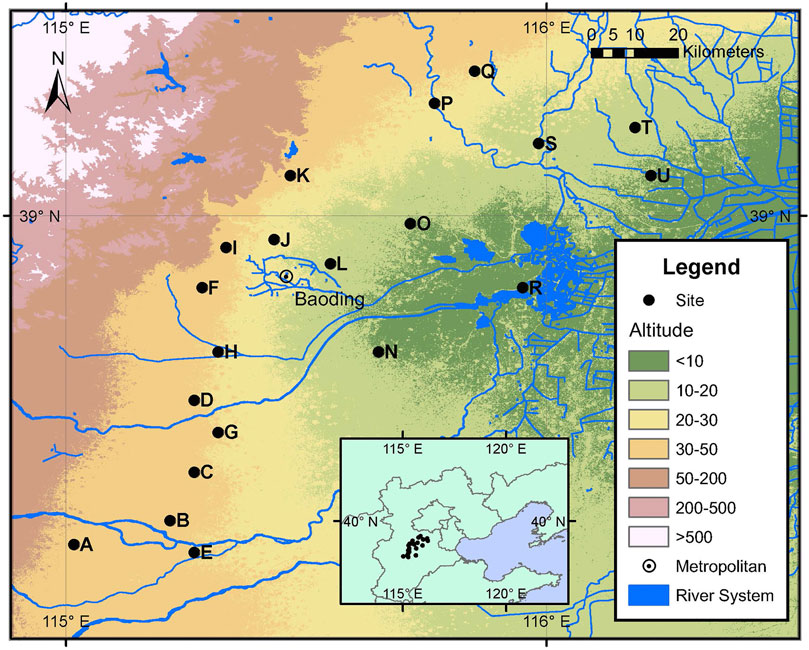
FIGURE 1. Location of all sites in the study area.

The study area mainly includes alluvial fans and alluvial plains, and the lithology is composed of gravels, sands, silts, and silty clays etc. Due to the scarcity of surface water resources in the study area, groundwater is the leading water resource. Agriculture and industries as a major grain producer and steel producer, respectively, in China, accounts for the most significant proportion of water consumption. Studies have shown that groundwater is almost the only source of irrigation water (Xiao et al., 2017). In addition, Hebei Province has historically been the largest steel-producing province in China, with a steel output of 2.184 billion tons in the past decade, accounting for 23% of the country’s total production. As a high water consumption industry, the development of the steel industries has contributed significantly to the depletion of groundwater in the region.

As shown in Figure 2, steel prices and API (Agricultural Price Index) negatively affect the depth of the water table. The three peaks appeared in 2005, 2009, and 2011, respectively, corresponding to the three valleys of the water table. Generally, the periods of high prices correspond to the periods of strong demand. In other words, during high prices, the production activities of steel and agriculture increased significantly, resulting in a large consumption of water, which in turn causes the water table to fall.

FIGURE 2

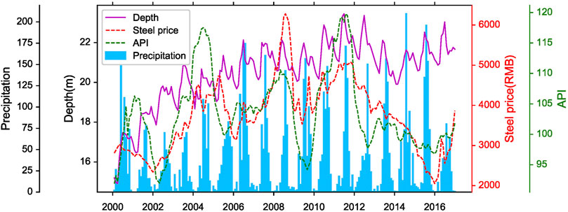
FIGURE 2. Comparison of the average water table depth and precipitation, steel price and API.

2.2 The LSTM Model

NN is a model that simulates the biological brain to achieve the artificial intelligence effect. The basic NN consists of an input layer, an output layer and a hidden layer. Each neuron is connected to the other by weights, and the training process is the process of updating weights. The NN activation function requires a nonlinear function that maps the input to a finite interval that determines whether the neuron is activated.

FNN is a simple NN that is widely used. All layers of the FNN are dense layers, and the parameters are propagated unidirectional from the input layer to the output layer and are updated by the error backpropagation algorithm. The NN parameters are the weights on each connection, and these weights are obtained by learning processes. Backpropagation algorithms based on the gradient descent method are often used to train NNs. In a NN, if we associate the hidden-layer state with each instant, we call it RNN. RNN is generally used for processing time series data because it uses information from the previous moment in each step. In this paper, the activation function we adopted between hidden layers is “tanh.” However, the calculations of the gradient of networks weight is essentially a continuous product operation. The gradients tend to zero or infinity exponentially with the length of the sequence increasing. It is the vanishing and exploding gradient problems. In this case, the model will ignore the previous state information. To solve this problem, the LSTM NN has been proposed (Hochreiter and Schmidhuber, 1997). A forget gate is added to the LSTM to manage the network’s “memory” to remember the model’s state for a long time. The following equation describes the computational procedure of LSTM:

$f_t=\sigma (b_f+U_f{s}_t+V_f{h}_{t-1})(1)$

$i_t=\sigma (b_i+U_i{s}_t+V_i{h}_{t-1})(2)$

$o_t=\sigma (b_o+U_o{s}_t+V_o{h}_{t-1})(3)$

$c_t=tanh(b_c+U_c{s}_t+V_c{h}_{t-1})(4)$

$m_t=f_t\otimes m_{t-1}+i_t\otimes c_t(5)$

where, c_t is calculated by s_t and h_t−1, forget gate and input gate are employed to control m_t. In RNN, h_t is the state of its hidden layer, while in LSTM, m_t (memory) is added to remember its long-term state and c_t to represent its cell state of the current input. In this study, “sigmoid” is employed as activation function of its forget gate.

2.3 Discrete Wavelet Transform

The idea of wavelet transform is to decompose the original sequence into different subsequences to provide detailed information about the multi-scale properties of time series. The superior function of wavelet transforms to reflect information on the time, location and frequency of a signal simultaneously (Cohen and Kovacevic, 1996). Wavelet transform is generally divided into continuous wavelet transform (CWT) and discrete wavelet transform (DWT). Due to information redundancy, DWT is usually recommended in hydrological forecasting (Quilty and Adamowski, 2018; Rajaee et al., 2019). Unlike CWT, DWT uses a specific subset of all zoom and translation values. In DWT, the original sequence is decomposed by a scale function for approximating the original sequence, and the wavelet function is used to describe the details of the original sequence. The scale function and wavelet function of the DWT decomposition can be defined as follows:

$\begin{array}{l}\hfill {\varphi }_{j,k}(t)=2^{j/2}\varphi (2^{j}t-k)\end{array}(6)$

$\begin{array}{l}\hfill {\psi }_{j,k}(t)=2^{j/2}\psi (2^{j}t-k)\end{array}(7)$

where ϕ(t) is scale function, ψ(t) is wavelet function, j and k are dilation factor and translation factor respectively.

Meanwhile, let V_j, W_j is a space spanned by ϕ_j,k(t), ψ_j,k(t) respectively, W_j is a orthogonal complement space of V_j:

$V_0=V_1\subset V_2\subset V_3\cdots \subset V_{j-1}\subset V_j\subset \cdots =W_{j-1}\oplus V_{j-1}(8)$

Thus, each V_j can be decompose to W_j−1 and V_j−1:

$V_j=W_{j-1}\oplus W_{j-2}\oplus W_{j-3}\oplus \cdots \oplus W_0\oplus V_0(9)$

In this study, DWT is applied to decompose the water table time series. The processed sub-time series are input to the LSTM model with meteorological data, socio-economic data as variables.

2.4 Data Processing

The input format of the LSTM or FNN is a multidimensional tensor. The input data is typically preprocessed in a three-dimensional tensor format like (samples, timesteps, features) for time series data. In this study, air temperature (K), precipitation (mm), evapotranspiration (mm) data, normalized difference vegetation index (NDVI) data, agricultural price index (API) and steel price data are harnessed as input variables of LSTM of FNN models. Air temperature, precipitation and evapotranspiration data in NetCDF (Network Common Data Form) format are resampled to monthly data. Monthly API and steel pricing data were collected from the website of the National Bureau of Statistics of China (http://www.stats.gov.cn/tjsj/), while Moderate Resolution Imaging Spectroradiometer (MODIS) provided NDVI data. Also, because the variables are different in order of magnitude, to make their scales uniform, the data has been normalised through the following equation to be a dimensionless value between 0 and 1:

$x_{scaled}=\frac{(x-x_{min})(max-min)}{(x_{max}-x_{min})}+min(10)$

where x_scaled is normalized data, x_min and x_max represent minimum and maximum value of the data respectively.

2.5 Model Evaluation

The NSE, RMSE (the root mean square error) and R (correlation coefficient) are harnessed to evaluate the performance of the model:

$\begin{array}{l}\hfill NSE=1-\frac{\sum _{i=1}^n{(O_i-P_i)}^2}{\sum _{i=1}^n{(O_i-\bar{O})}^2}\end{array}(11)$

$\begin{array}{l}\hfill RMSE=\sqrt{\frac{\sum _{i=1}^n{(O_i-P_i)}^2}{n}}\end{array}(12)$

$\begin{array}{l}\hfill R=\frac{\sum _{i=1}^n(O_i-\bar{O})(P_i-\bar{P})}{\sqrt{\left[\sum _{i=1}^n{(O_i-\bar{O})}^2\right]\left[\sum _{i=1}^n{(P_i-\bar{P})}^2\right]}}\end{array}(13)$

where O_i is observed value at time i, P_i is predicted value at time i, $\bar{O}$ is the mean value of O_i, $\bar{P}$ is the mean value of P_i. The NSE value range from negative infinity to 1 while the correlation coefficient R from −1 to 1. The prediction is ideal if NSE and correlation coefficient are close to 1 or RMSE to 0.

3 Results and Discussions

3.1 The LSTM Model

The correlation between the two sites was examined to reduce the noise influence of the water table data as much as possible. According to the correlated heat map of the water table depth at each site (Figure 3), the 20 sites are divided into four clusters (Figure 4). Data from the first 14 years is used for training purposes, and the data from the next 3 years is used for testing purposes. As each cluster, model’s output represents the water table depth prediction of all sites included in this cluster.

FIGURE 3

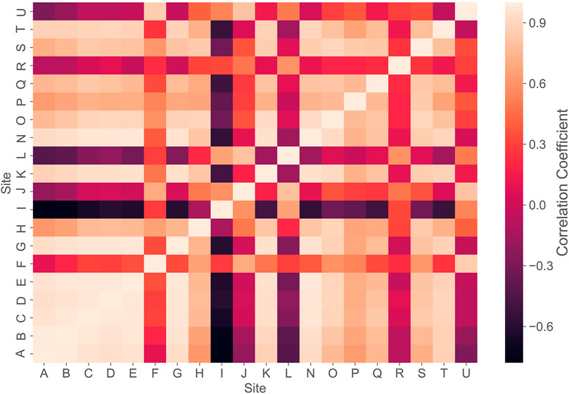
FIGURE 3. Correlation heatmap of all sites.

FIGURE 4

FIGURE 4. Clustering of all sites.

Table 1 shows the NSE, RMSE, and correlation coefficients of all sites during the training and testing periods using the LSTM model and wavelet-LSTM model. It is evident that the NSE of all sites during the training period is greater than 0.8, and the correlation coefficients are greater than 0.9. During the testing period, the NSE at all sites was significantly lower than the NSE during the training period and was even negative at sites J, K, R, and S. The results indicate that quite a significant overfitting phenomenon occurs. From a spatial point of view, the simulation performance of the densely distributed area (cluster 1) is better, while the sparsely distributed area (cluster 4) has poor simulation performance. In addition, the closer to the lake, the weaker the results are. It may be due to the fact that the water table depth near the lake is strongly affected by the lake. However, hydrological data for the lake is lacking.

TABLE 1

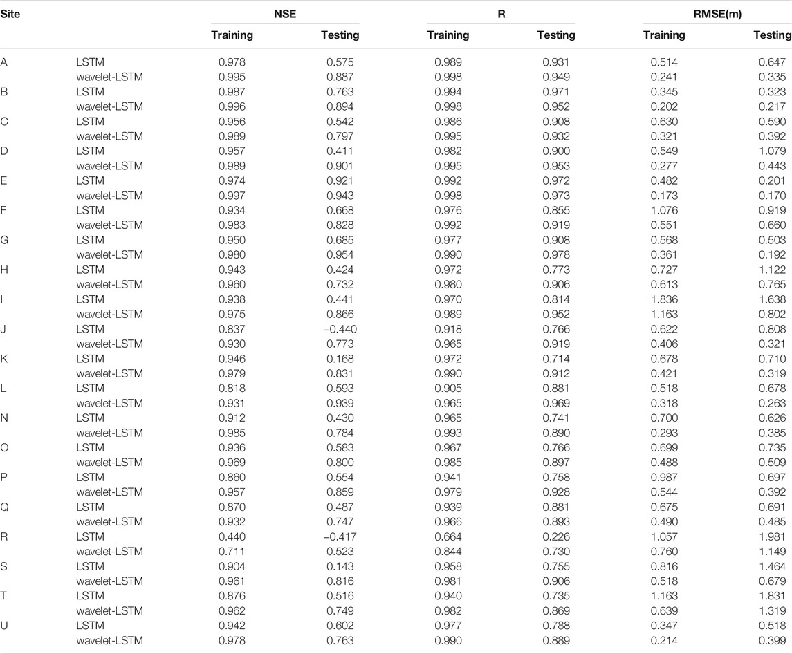
TABLE 1. Comparison of performance between LSTM model and wavelet-LSTM model.

3.2 The Wavelet-LSTM Model

The processed sub-time series decomposed using wavelets is used as the input of the LSTM model to improve the output. On the selection of wavelet function, Daubechies family wavelet (dbN, N refers to the number of vanishing moments) (Khan et al., 2020) and Meyer wavelet (Freire et al., 2019)are commonly used; Haar wavelet are also often used for comparative studies (Liu et al., 2012; Ebrahimi and Rajaee, 2017).

Maheswaran and Khosa (2012) proposed that a wavelet with a compact support is suitable for processing time series with short memory with short-duration transient features while wavelets with wider support for time series with long term features. Nourani et al. (2009) used db4 and Meyer wavelet to decompose the time series with two decomposition levels to simulate monthly precipitation data. Gorgij et al. (2017) used a db4 wavelet to decompose the monthly water table data with two levels. Nanda et al. (2019) used a db2 wavelet to decompose the daily time series with five levels to simulate the daily streamflow data. Therefore, the wavelet function and levels of decomposition should be carefully determined according to different conditions.

In this study, db2, db4, and Meyer wavelet are used for comparison. The NSE value of the three wavelets used by the model in the testing phase are shown in Figure 5. It can be seen that although db2 and db4 wavelets may be close or even slightly better than Meyer wavelet at some sites, the advantages of Meyer wavelets are evident on most sites. It should be noted that, as wavelet components are input into the model as variables, the decomposition level could not be unduly high. Because it is not practical to apply the network effectively when the number of training samples is limited while the dimension of the feature space is large (Liu et al., 2017). The sub-time series of the data of site A decomposed by Meyer wavelets are shown in Figure 6. The component d₃ (three decomposition levels) can be seen to have a significant periodic variation feature. As a result, three levels of decomposition were used.

FIGURE 5

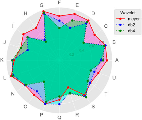
FIGURE 5. NSE value of three models using db2, db4, and meyer wavelet respectively.

FIGURE 6

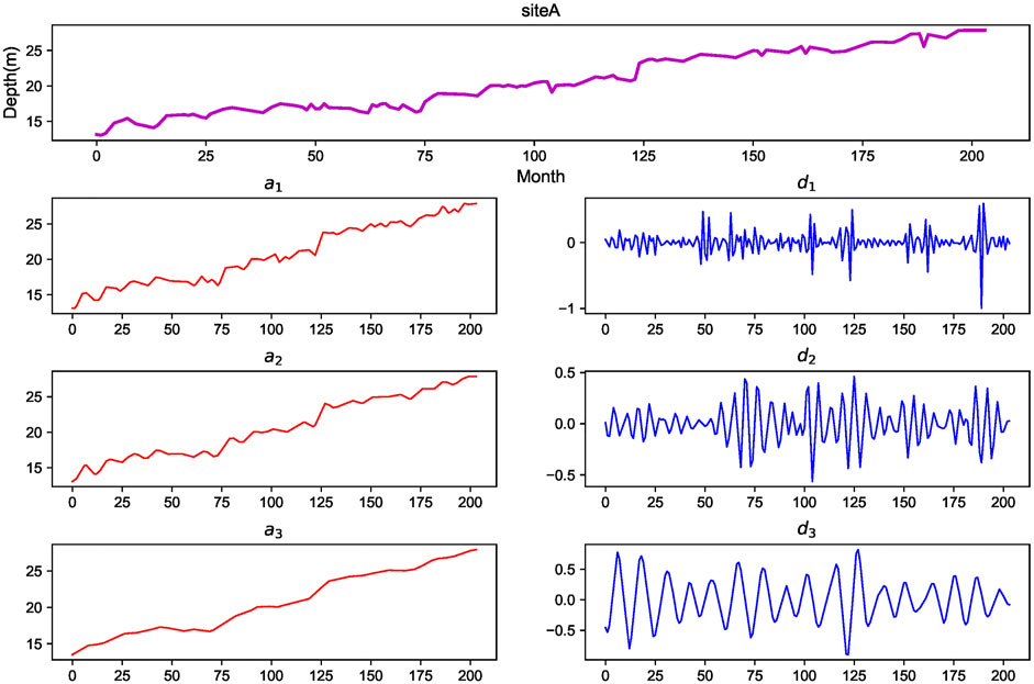
FIGURE 6. Decomposition of the time series of site A.

As shown in Table 1, the performance of the wavelet-LSTM model is significantly better than that of the single LSTM model. The simulation results of both models during training and testing periods are shown in Figure 7. During the training period, the LSTM model without wavelet transform does not accurately simulate the water table under extreme conditions (peaks and troughs) and is subject to overfitting during the testing process. For example, when a single LSTM model is used, the NSE value for sites J, K, and S are 0.837, 0.946, and 0.904, respectively, while in the testing phase, the NSE value are −0.440, 0.168, and 0.143, respectively. After using the wavelet-LSTM model, the NSE value reached 0.773, 0.831, and 0.816, respectively for sites J, K, and S. It should be noted that site R is close to Baiyangdian Lake, the study area’s primary surface water body. Despite the lacking of hydrological data for Baiyangdian Lake, utilizing the wavelet-LSTM model enhanced the simulation effect of the R site from −0.417 to 0.523. The results indicate that the phenomenon of overfitting was significantly improved. From the comparison of Figures 8A,B, it can be seen that compared to a single LSTM, the simulation effect of each site has been considerably improved under the LSTM model coupled by wavelets. The delayed response of water table depth data to weather conditions and our inability to obtain socio-economic data with higher spatial resolution makes it impossible to use a single LSTM model to capture the exact characteristics of the water table series accurately. However, the wavelet transform is very suitable for dealing with the non-stationary and stochastic nature of groundwater variability.

FIGURE 7

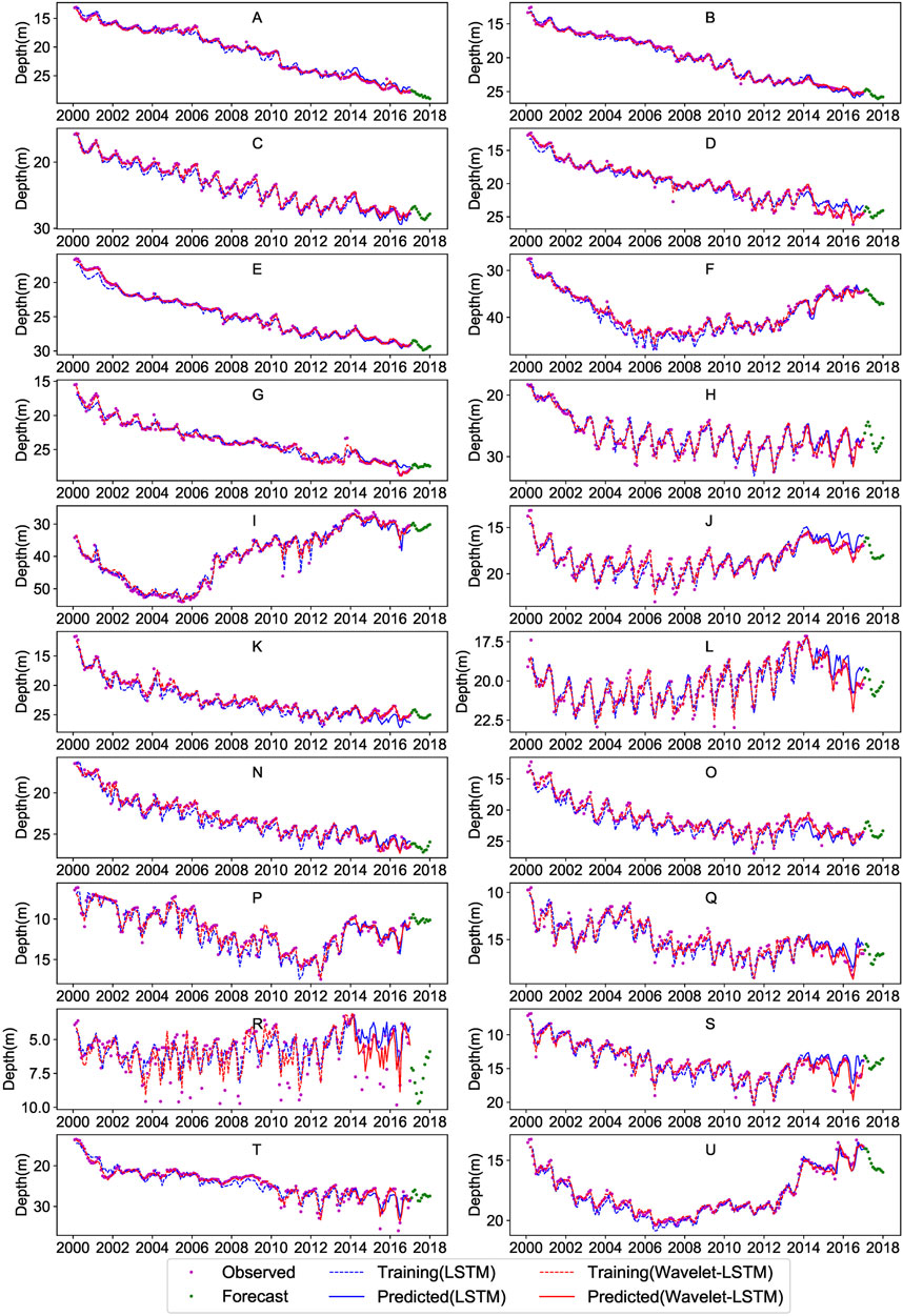
FIGURE 7. Comparison of observed, simulated and forecast water table depth applied the single LSTM model and the wavelet-LSTM model at each site.

FIGURE 8

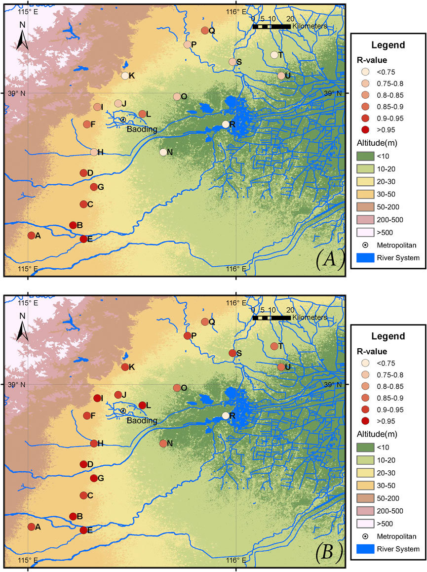
FIGURE 8. Spatial distribution of R values using LSTM model and wavelet-LSTM model during the testing period: (A) LSTM (B) wavelet-LSTM.

As described in Section 2.2, unlike LSTM-NNs, FNN has no memory and cannot record the state of individual inputs. Therefore, the wavelet transform is combined with FNN (wavelet-FNN) and compared with wavelet-LSTM on the water table forecasting effect. Figure 9 shows the RMSE comparison of the combined wavelet transform with FNN and LSTM-NN over the next 1–12 months. As expected, FNN is not as efficient as the LSTM model for time series data. Although the RMSE increases with prediction time increases, wavelet-LSTM still performs better than wavelet-FNN simulation for almost all sites. This phenomenon is more evident as the prediction time increases, reflecting the features of the wavelet-LSTM, which can memorise information for a long time.

FIGURE 9

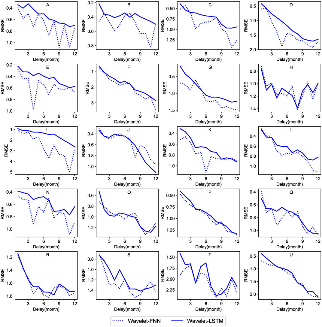
FIGURE 9. Comparison of RMSE values of water table depth using wavelet-LSTM and wavelet-FNN models with 1–12 months delays.

It should be noted that the underground funnels are mainly distributed in the southwest of the study area, namely sites A, B, C, D, E, and G. For these sites, the advantages of wavelet-LSTM are particularly evident, and the RMSE of wavelet-LSTM is even less than half of wavelet-FNN in individual sites, illustrating the applicability of wavelet-LSTM in overexploited areas. Therefore, it can be concluded that LSTM-NN is better than FNN in long-term prediction in areas where anthropogenic activities strongly influence groundwater. It further shows that the wavelet-LSTM model can effectively simulate the non-stationary water table variation in the overexploited area.

3.3 Forecast of the Future Water Table Depth

Given that meteorological data, socio-economic data are unknown, we need to use the present value of these parameters at this time to forecast the water table depth for the unknown future. To predict the value of weather data, socio-economic and other variable data for the unknown future, we need to use the present value of these parameters at this time. To ensure as much precision as possible, we respectively use the wavelet-LSTM model with a delay of 1–12 months to predict the water table depth in the next 1–12 months. The green dotted line indicates the results of the future predictions (Figure 7). Figure 10 compares correlation coefficient R values between the LSTM model and wavelet-LSTM model during the delayed testing period for 1–12 months. Although the R values decrease as the prediction delay increases, the performance of wavelet-LSTM is remarkably better than the single LSTM model in 6 months’ prediction, as expected. Wavelet-LSTM also shows higher stability.

FIGURE 10

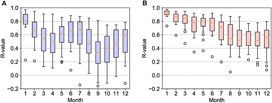
FIGURE 10. Comparison of R values between LSTM model and wavelet-LSTM model during the testing period for 1–12 months forecast: (A) LSTM (B) wavelet-LSTM.

Furthermore, the results show that for a single LSTM model, the 6-months forecast is sometimes more reliable than the 4 or 5-months forecast. However, the former has a longer time frame; the 12-months forecast shows better than 9, 10 or 11 months of superior performance. Nevertheless, for wavelet-LSTM, the advantages in the 6 and 12 months forecasts are not obvious. In other words, wavelet transform increases the model’s dependence on the autocorrelation of the data.

In addition, to evaluate the response of groundwater to changes in various variables (such as climate change, economic development, etc.) in the future, future simulated values of these variables are entered into the model. Then the recursive method is used to predict the water table depth in the future gradually. Figure 11 shows the 12-months recursive forecast using the January 2016 forecast values. In this method, the meteorological and socio-economic data are real values, and the wavelet decomposition data will be predicted and produced simultaneously with the water table depth data. It can be seen that the losses of most sites have not increased significantly over time. Mainly at sites B, E, and L, the RMSE values reached 0.090, 0.059, and 0.218 m, respectively. The prediction curve and the observation curve can be matched precisely. The results show the effectiveness of this method for predicting and evaluating the water table.

FIGURE 11

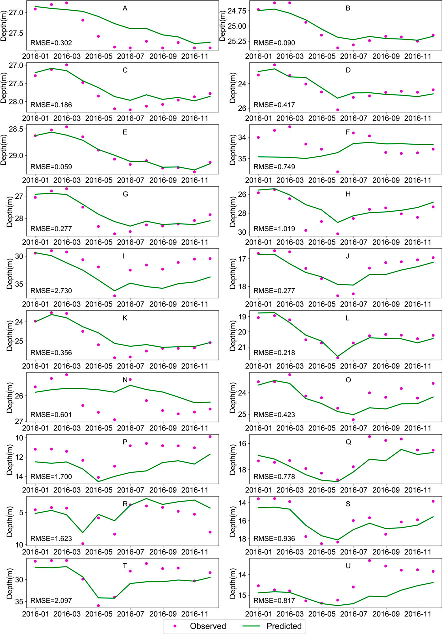
FIGURE 11. Recursive prediction using wavelet-LSTM model for 1–12 months.

3.4 Importance Evaluation of Each Variable

To evaluate the impact of each variable on the simulation effect, we calculate the contribution of each node in the following equation:

$\left(\begin{array}{cccc}\hfill C_1\hfill & \hfill \dots \hfill & \hfill C_j\dots \hfill & \hfill C_n\hfill \end{array}\right)=\left(\begin{array}{cccc}\hfill R_1\hfill & \hfill \dots \hfill & \hfill R_j\dots \hfill & \hfill R_m\hfill \end{array}\right)\left(\begin{array}{ccccc}\hfill w_{11}\hfill & \hfill \dots \hfill & \hfill w_{1j}\hfill & \hfill \dots \hfill & \hfill w_{1n}\hfill \\ \hfill \dots \hfill & \hfill \hfill & \hfill \hfill & \hfill \hfill & \hfill \dots \hfill \\ \hfill w_{i1}\hfill & \hfill \dots \hfill & \hfill w_{1j}\hfill & \hfill \dots \hfill & \hfill w_{in}\hfill \\ \hfill \dots \hfill & \hfill \hfill & \hfill \hfill & \hfill \hfill & \hfill \dots \hfill \\ \hfill w_{m1}\hfill & \hfill \dots \hfill & \hfill w_{mj}\hfill & \hfill \dots \hfill & \hfill w_{mn}\hfill \end{array}\right)(14)$

where C_j represents the contribution of the j node to the results; R_i represents the correlation coefficient of prediction value and the measured value at i-th site (Table 1); w_ij represents the input layer weight of the i-th site, the j-th node.

As shown in Figure 12, a₃, d₁, d₂, d₃ represent wavelet decomposition sequence; L_t−1 represents the past water table; temp represents temperature; et0 represents evapotranspiration; prec represents precipitation. The approximate component (a₃) of the wavelet has the greatest impact, accounting for 18.4% of the total contribution; then, the past water level (L_t−1) can explain 13.4% of the result. Among the external variables, precipitation and evapotranspiration have the greatest impact on the results through recharge, vegetation and soil evapotranspiration. The steel price contribution rate is 7.3%, slightly higher than NDVI and API. It fully shows that agricultural irrigation and climate change will affect groundwater, but the steel industry, the mainstay industry in the study area, also has a big impact on groundwater. The prices of agricultural products are also affected by meteorological conditions. For example, precipitation can increase the yield of crops such as corn, but it is harmful to cotton (Eck et al., 2020). However, increased agricultural production can also lead to a drop in the water table due to increased irrigation. Consequently, the contribution rate of agriculture is lower than that of industry.

FIGURE 12

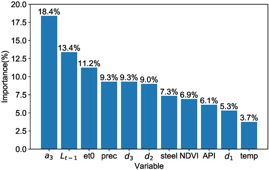
FIGURE 12. Importance percentage of each variable.

Since the wavelet components and past water table depth data accounted for more than 50% percent of the weights. If the remaining variables are considered “external variables,” the weights of the socio-economic factors (price of steel, API and NDVI) represent almost half of the external variables. Figure 13 shows the impact of the temperature, precipitation, evaporation, API, steel price and NDVI on the water table in 20 sites, respectively. For most sites, precipitation and evaporation contribute to changes in the water table, and evaporation at site E and precipitation at site D was even more than half. While the weight of the price of steel and API is not as great as precipitation and evaporation, it is still considerable. Site D has the lowest socio-economic impact, and the weight is less than 1/3. However, the socio-economic ratio of most sites is in the range of 1/2–1/3.

FIGURE 13

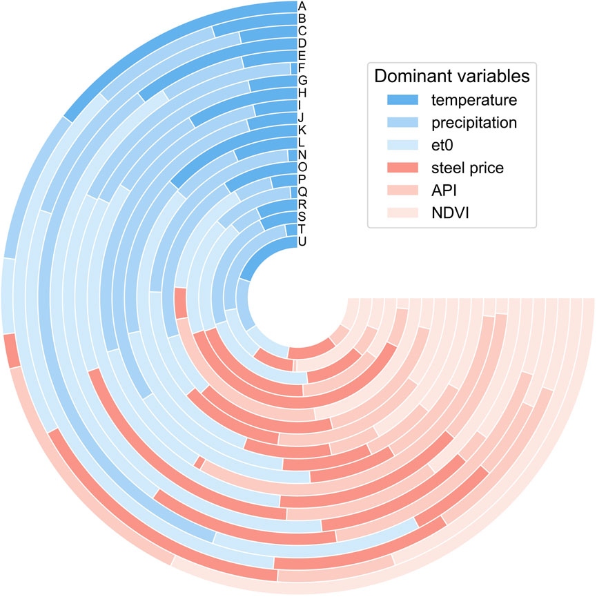
FIGURE 13. Impact of dominant variables on water table depth at each site.

It should be noted that it is unavoidable for socio-economic data to exhibit extreme price swings caused by emotional investment decisions. For example, due to the impact of the 2008 financial crisis, the steel price index fell sharply. In this case, water table fluctuation cannot accurately reflect the relationship between supply and demand. As a result, we strive to reflect the degree of influence of each element using the model.

In addition, this study also analysed the dominant factors affecting the water table by land use distribution. Most of the study area is occupied by agricultural land, forest and pastures. A large portion of industrial land is distributed northwest of Baoding city, close to the forest. According to surveys, the leading industry in northwest Baoding is papermaking, which consumes a lot of water and wood. Since the variables are not independent, we also used anthropogenic activities and meteorological ratios as much as possible to describe the relationship of each variable. The lower the ratio, the greater the impact of anthropogenic activities (Figure 14). It can be seen that except for P, Q, and R, the ratio of all sites are greater than 1. Since the R is close to Baiyangdian Lake, its water table is heavily influenced by human activities, fluctuates erratically and the simulation impact is weak. This outcome is also consistent with the study of Gorgij et al. (2017). They found that the sites located on the river may be affected by the fluctuations in the river water and that the simulation effect of these sites is not as good as that of other sites. In addition, the water table depth of P and Q are strongly affected by anthropogenic activities. Site A, B, C, D, E, and G in the southwest of the study region are the central over mining areas. Except for the points near C and D, fewer industries and the proportion of agricultural land is relatively large. The water table of these sites have trended downward and are greatly affected by anthropogenic activities. In this regard, Dong et al. (2019) concluded that the water table dropped most significantly in the place with the highest proportion of agricultural land.

FIGURE 14

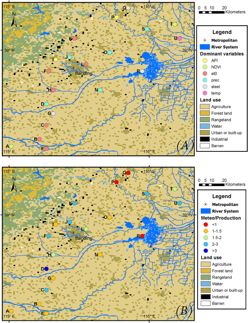
FIGURE 14. The relationship between land use and importance of variables: (A) Dominant variables at each site (B) The ratio of meteorological factors to production activity factors.

The water table in the study area shows a downward trend from A, B, C, D, E, G, H, K, N, and O, located in the southwestern part of the study region, while this is where the groundwater funnel area is located. It may be because the southwest of the study area is dominated by agricultural land and far away from industrial areas and lakes. As the main crop in this region, the price of wheat per unit of yield is relatively stable, and the water table trend has not changed significantly. At these sites, the ratio of meteorological to human activity weights for A, B, E, G, N, and O is 1–1.5, and D is 3. Other sites (F, I, J, K, l, P, Q, R, S, T, U) showed a decrease then and increase, or complicated fluctuations. These sites are mainly distributed in the north of the study area. Among these sites, the ratio of meteorological to human activity weights for sites I, P, Q, and R are relatively low, while F, K, J, L, S, T, and U sites show high ratios. Since the effects of various variables on groundwater are not independent, agricultural production is also affected by meteorological changes. Therefore, these two regions consist of sites with higher meteorological weights and sites with lower meteorological weights. However, in general, the sites with lower meteorological weight are mainly distributed in the groundwater funnel area.

4 Conclusion

This study evaluated the predictive performance of the LSTM combined with wavelet transform in the groundwater over-exploitation region. The results show that the NN can be used as an efficient model for prediction. Moreover, due to anthropogenic activities, the data is rich in noise and non-stationary in the groundwater over-exploitation area. The original sequence is decomposed into three levels by Meyer wavelet, which can significantly improve the simulation effect of LSTM. Using the wavelet transform combined with LSTM and FNN to predict the water table depth over the next 1–12 months, it can be concluded that the long-term prediction effect of LSTM-NN in areas of over-exploitation of groundwater is better than FNN, indicating that LSTM can memorise long-term information and effectively understand bit trend changes in water table. Furthermore, by using meteorological and socio-economic data, the proposed model can forecast future changes in the water table through a recursive method, providing a benchmark for rational utilisation planning of groundwater.

In addition, the contribution of various variables on the water table can be analysed through the LSTM-NN. The results show that Baoding’s steel industry has a greater impact on water table changes. Moreover, the contribution of anthropogenic activities is higher in the sites close to the surface water. It shows that agricultural irrigation water can affect the water table. However, industrial production contributes to lowering the water table, especially in the study area where secondary industry represents a relatively large proportion. The simulation results can provide scientific guidance for the rational development and utilisation of groundwater resources in the study area.

However, we can still find that our interpretation of the variables is vague due to the nature of the NN black-box model. Therefore, more parameters, such as groundwater pumping data, should be considered in future research. If possible, in the subsequent application of the model, the amount of data should be further increased. Data that directly affects the water table should be collected, such as water pumping, crop yields, etc.

Data Availability Statement

The datasets presented in this article are not readily available because legal and policy restrictions. Requests to access the datasets should be directed to HH, huhongchang@tsinghua.edu.cn.

Author Contributions

ZL performed the study and wrote the manuscript. YL and HH designed the study and revised the manuscript. HL, YM, and MK revised the manuscript. All authors approved the publication of the final manuscript.

Funding

The research was funded by the National Key R&D Program of China (2018YFC1508103, 2018YFC1508102), the National Natural Science Foundation of China (51879136, 51809173, 41930109).

Conflict of Interest

The authors declare that the research was conducted in the absence of any commercial or financial relationships that could be construed as a potential conflict of interest.

Publisher’s Note

All claims expressed in this article are solely those of the authors and do not necessarily represent those of their affiliated organizations, or those of the publisher, the editors and the reviewers. Any product that may be evaluated in this article, or claim that may be made by its manufacturer, is not guaranteed or endorsed by the publisher.

References

Adamowski, J., and Sun, K. (2010). Development of a Coupled Wavelet Transform and Neural Network Method for Flow Forecasting of Non-perennial Rivers in Semi-arid Watersheds. J. Hydrol. 390, 85–91. doi:10.1016/j.jhydrol.2010.06.033

CrossRef Full Text | Google Scholar

Altunkaynak, A. (2007). Forecasting Surface Water Level Fluctuations of lake Van by Artificial Neural Networks. Water Resour. Manage. 21, 399–408. doi:10.1007/s11269-006-9022-6

CrossRef Full Text | Google Scholar

Chang, F.-J., Chen, P.-A., Lu, Y.-R., Huang, E., and Chang, K.-Y. (2014). Real-time Multi-Step-Ahead Water Level Forecasting by Recurrent Neural Networks for Urban Flood Control. J. Hydrol. 517, 836–846. doi:10.1016/j.jhydrol.2014.06.013

CrossRef Full Text | Google Scholar

Chen, L.-H., Chen, C.-T., and Pan, Y.-G. (2010). Groundwater Level Prediction Using SOM-RBFN Multisite Model. J. Hydrologic Eng. doi:10.1061/(asce)he.1943-5584.0000218

CrossRef Full Text | Google Scholar

Chen, X., Wang, P., Muhammad, T., Xu, Z., and Li, Y. (2020). Subsystem-level Groundwater Footprint Assessment in North China Plain - the World's Largest Groundwater Depression Cone. Ecol. Indicators 117, 106662. doi:10.1016/j.ecolind.2020.106662

CrossRef Full Text | Google Scholar

Cohen, A., and Kovacevic, J. (1996). Wavelets: The Mathematical Background. Proc. IEEE 84, 514–522. doi:10.1109/5.488697

CrossRef Full Text | Google Scholar

Coppola, E., Szidarovszky, F., Poulton, M., and Charles, E. (2003). Artificial Neural Network Approach for Predicting Transient Water Levels in a Multilayered Groundwater System under Variable State, Pumping, and Climate Conditions. J. Hydrologic Eng. doi:10.1061/(asce)1084-0699(2003)8:6(348)

CrossRef Full Text | Google Scholar

Coulibaly, P., Anctil, F., Aravena, R., and Bobée, B. (2001). Artificial Neural Network Modeling of Water Table Depth Fluctuations. Water Resour. Res. 37, 885–896. doi:10.1029/2000WR900368

CrossRef Full Text | Google Scholar

Daliakopoulos, I. N., Coulibaly, P., and Tsanis, I. K. (2005). Groundwater Level Forecasting Using Artificial Neural Networks. J. Hydrol. 309, 229–240. doi:10.1016/j.jhydrol.2004.12.001

CrossRef Full Text | Google Scholar

Daubechies, I. (1990). The Wavelet Transform, Time-Frequency Localization and Signal Analysis. IEEE Trans. Inform. Theor. 36, 961–1005. doi:10.1109/18.57199

CrossRef Full Text | Google Scholar

de Vos, N. J., and Rientjes, T. H. M. (2005). Constraints of Artificial Neural Networks for Rainfall-Runoff Modelling: Trade-Offs in Hydrological State Representation and Model Evaluation. Hydrol. Earth Syst. Sci. 9, 111–126. doi:10.5194/hess-9-111-2005

CrossRef Full Text | Google Scholar

Dong, Y., Jiang, C., Suri, M. R., Pee, D., Meng, L., and Rosenberg Goldstein, R. E. (2019). Groundwater Level Changes with a Focus on Agricultural Areas in the Mid-Atlantic Region of the United States, 2002-2016. Environ. Res. 171, 193–203. doi:10.1016/j.envres.2019.01.004

PubMed Abstract | CrossRef Full Text | Google Scholar

Ebrahimi, H., and Rajaee, T. (2017). Simulation of Groundwater Level Variations Using Wavelet Combined with Neural Network, Linear Regression and Support Vector Machine. Glob. Planet. Change 148, 181–191. doi:10.1016/j.gloplacha.2016.11.014

CrossRef Full Text | Google Scholar

Eck, M. A., Murray, A. R., Ward, A. R., and Konrad, C. E. (2020). Influence of Growing Season Temperature and Precipitation Anomalies on Crop Yield in the southeastern United States. Agric. For. Meteorology 291, 108053. doi:10.1016/j.agrformet.2020.108053

CrossRef Full Text | Google Scholar

Freire, P. K. d. M. M., Santos, C. A. G., and Silva, G. B. L. d. (2019). Analysis of the Use of Discrete Wavelet Transforms Coupled with ANN for Short-Term Streamflow Forecasting. Appl. Soft Comput. 80, 494–505. doi:10.1016/j.asoc.2019.04.024

CrossRef Full Text | Google Scholar

Gong, H., Pan, Y., Zheng, L., Li, X., Zhu, L., Zhang, C., et al. (2018). Long-term Groundwater Storage Changes and Land Subsidence Development in the North China Plain (1971-2015). Hydrogeol J. 26, 1417–1427. doi:10.1007/s10040-018-1768-4

CrossRef Full Text | Google Scholar

Gorgij, A. D., Kisi, O., and Moghaddam, A. A. (2017). Groundwater Budget Forecasting, Using Hybrid Wavelet-ANN-GP Modelling: A Case Study of Azarshahr Plain, East Azerbaijan, Iran. Hydrol. Res. 48, 455–467. doi:10.2166/nh.2016.202

CrossRef Full Text | Google Scholar

Hewage, P., Trovati, M., Pereira, E., and Behera, A. (2021). Deep Learning-Based Effective fine-grained Weather Forecasting Model. Pattern Anal. Applic 24, 343–366. doi:10.1007/s10044-020-00898-1

CrossRef Full Text | Google Scholar

Hochreiter, S., and Schmidhuber, J. (1997). Long Short-Term Memory. Neural Comput. 9, 1735–1780. doi:10.1162/neco.1997.9.8.1735

PubMed Abstract | CrossRef Full Text | Google Scholar

Huang, J., Zhou, Y., Wenninger, J., Ma, H., Zhang, J., and Zhang, D. (2016). How Water Use of Salix Psammophila bush Depends on Groundwater Depth in a Semi-desert Area. Environ. Earth Sci. 75. doi:10.1007/s12665-016-5376-0

CrossRef Full Text | Google Scholar

Khan, M. M. H., Muhammad, N. S., and El-Shafie, A. (2020). Wavelet Based Hybrid ANN-ARIMA Models for Meteorological Drought Forecasting. J. Hydrol. 590, 125380. doi:10.1016/j.jhydrol.2020.125380

CrossRef Full Text | Google Scholar

Kim, T.-W., and Valdés, J. B. (2003). Nonlinear Model for Drought Forecasting Based on a Conjunction of Wavelet Transforms and Neural Networks. J. Hydrologic Eng. doi:10.1061/(asce)1084-0699(2003)8:6(319)

CrossRef Full Text | Google Scholar

Kratzert, F., Klotz, D., Brenner, C., Schulz, K., and Herrnegger, M. (2018). Rainfall-runoff Modelling Using Long Short-Term Memory (LSTM) Networks. Hydrol. Earth Syst. Sci. 22, 6005–6022. doi:10.5194/hess-22-6005-2018

CrossRef Full Text | Google Scholar

Lachaal, F., Mlayah, A., Bédir, M., Tarhouni, J., and Leduc, C. (2012). Implementation of a 3-D Groundwater Flow Model in a Semi-arid Region Using MODFLOW and GIS Tools: The Zéramdine-Béni Hassen Miocene Aquifer System (East-central Tunisia). Comput. Geosciences 48, 187–198. doi:10.1016/j.cageo.2012.05.007

CrossRef Full Text | Google Scholar

Li, J., Wang, Y., Zhu, C., Xue, X., Qian, K., Xie, X., et al. (2020). Hydrogeochemical Processes Controlling the Mobilization and Enrichment of Fluoride in Groundwater of the North China Plain. Sci. Total Environ. 730, 138877. doi:10.1016/j.scitotenv.2020.138877

PubMed Abstract | CrossRef Full Text | Google Scholar

Liu, P., Zhang, H., and Eom, K. B. (2017). Active Deep Learning for Classification of Hyperspectral Images. IEEE J. Sel. Top. Appl. Earth Observations Remote Sensing 10, 712–724. doi:10.1109/JSTARS.2016.2598859

CrossRef Full Text | Google Scholar

Liu, Z., Peng, C., Xiang, W., Deng, X., Tian, D., Zhao, M., et al. (2012). Simulations of Runoff and Evapotranspiration in Chinese Fir Plantation Ecosystems Using Artificial Neural Networks. Ecol. Model. 226, 71–76. doi:10.1016/j.ecolmodel.2011.11.023

CrossRef Full Text | Google Scholar

Maheswaran, R., and Khosa, R. (2012). Comparative Study of Different Wavelets for Hydrologic Forecasting. Comput. Geosciences 46, 284–295. doi:10.1016/j.cageo.2011.12.015

CrossRef Full Text | Google Scholar

Maihemuti, B., Simayi, Z., Alifujiang, Y., Aishan, T., Abliz, A., and Aierken, G. (2021). Development and Evaluation of the Soil Water Balance Model in an Inland Arid delta Oasis: Implications for Sustainable Groundwater Resource Management. Glob. Ecol. Conservation 25, e01408. doi:10.1016/j.gecco.2020.e01408

CrossRef Full Text | Google Scholar

Mohanty, S., Jha, M. K., Kumar, A., and Panda, D. K. (2013). Comparative Evaluation of Numerical Model and Artificial Neural Network for Simulating Groundwater Flow in Kathajodi-Surua Inter-basin of Odisha, India. J. Hydrol. 495, 38–51. doi:10.1016/j.jhydrol.2013.04.041

CrossRef Full Text | Google Scholar

Nanda, T., Sahoo, B., Beria, H., and Chatterjee, C. (2016). A Wavelet-Based Non-linear Autoregressive with Exogenous Inputs (WNARX) Dynamic Neural Network Model for Real-Time Flood Forecasting Using Satellite-Based Rainfall Products. J. Hydrol. 539, 57–73. doi:10.1016/j.jhydrol.2016.05.014

CrossRef Full Text | Google Scholar

Nanda, T., Sahoo, B., and Chatterjee, C. (2019). Enhancing Real-Time Streamflow Forecasts with Wavelet-Neural Network Based Error-Updating Schemes and ECMWF Meteorological Predictions in Variable Infiltration Capacity Model. J. Hydrol. 575, 890–910. doi:10.1016/j.jhydrol.2019.05.051

CrossRef Full Text | Google Scholar

Nayak, P. C., Rao, Y. R. S., and Sudheer, K. P. (2006). Groundwater Level Forecasting in a Shallow Aquifer Using Artificial Neural Network Approach. Water Resour. Manage. 20, 77–90. doi:10.1007/s11269-006-4007-z

CrossRef Full Text | Google Scholar

Nourani, V., Alami, M. T., and Aminfar, M. H. (2009). A Combined Neural-Wavelet Model for Prediction of Ligvanchai Watershed Precipitation. Eng. Appl. Artif. Intelligence 22, 466–472. doi:10.1016/j.engappai.2008.09.003

CrossRef Full Text | Google Scholar

Nourani, V., and Mousavi, S. (2016). Spatiotemporal Groundwater Level Modeling Using Hybrid Artificial Intelligence-Meshless Method. J. Hydrol. 536, 10–25. doi:10.1016/j.jhydrol.2016.02.030

CrossRef Full Text | Google Scholar

Quilty, J., and Adamowski, J. (2018). Addressing the Incorrect Usage of Wavelet-Based Hydrological and Water Resources Forecasting Models for Real-World Applications with Best Practices and a New Forecasting Framework. J. Hydrol. 563, 336–353. doi:10.1016/j.jhydrol.2018.05.003

CrossRef Full Text | Google Scholar

Rajaee, T., Ebrahimi, H., and Nourani, V. (2019). A Review of the Artificial Intelligence Methods in Groundwater Level Modeling. J. Hydrol. 572, 336–351. doi:10.1016/j.jhydrol.2018.12.037

CrossRef Full Text | Google Scholar

Roy, P. K., Roy, S. S., Giri, A., Banerjee, G., Majumder, A., and Mazumdar, A. (2015). Study of Impact on Surface Water and Groundwater Around Flow fields Due to Changes in River Stage Using Groundwater Modeling System. Clean. Techn Environ. Pol. 17, 145–154. doi:10.1007/s10098-014-0769-9

CrossRef Full Text | Google Scholar

Tang, Q., Zhang, X., and Tang, Y. (2013). Anthropogenic Impacts on Mass Change in North China. Geophys. Res. Lett. 40, 3924–3928. doi:10.1002/grl.50790

CrossRef Full Text | Google Scholar

Taormina, R., Chau, K.-w., and Sethi, R. (2012). Artificial Neural Network Simulation of Hourly Groundwater Levels in a Coastal Aquifer System of the Venice Lagoon. Eng. Appl. Artif. Intelligence 25, 1670–1676. doi:10.1016/j.engappai.2012.02.009

CrossRef Full Text | Google Scholar

Tiwari, M. K., and Chatterjee, C. (2010). Development of an Accurate and Reliable Hourly Flood Forecasting Model Using Wavelet-Bootstrap-ANN (WBANN) Hybrid Approach. J. Hydrol. 394, 458–470. doi:10.1016/j.jhydrol.2010.10.001

CrossRef Full Text | Google Scholar

Xiang, Z., Bailey, R. T., Nozari, S., Husain, Z., Kisekka, I., Sharda, V., et al. (2020). DSSAT-MODFLOW: A New Modeling Framework for Exploring Groundwater Conservation Strategies in Irrigated Areas. Agric. Water Manag. 232, 106033. doi:10.1016/j.agwat.2020.106033

CrossRef Full Text | Google Scholar

Xiao, D., Shen, Y., Qi, Y., Moiwo, J. P., Min, L., Zhang, Y., et al. (2017). Impact of Alternative Cropping Systems on Groundwater Use and Grain Yields in the North China Plain Region. Agric. Syst. 153, 109–117. doi:10.1016/j.agsy.2017.01.018

CrossRef Full Text | Google Scholar

Xu, X., Huang, G., Zhan, H., Qu, Z., and Huang, Q. (2012). Integration of SWAP and MODFLOW-2000 for Modeling Groundwater Dynamics in Shallow Water Table Areas. J. Hydrol. 412-413, 170–181. doi:10.1016/j.jhydrol.2011.07.002

CrossRef Full Text | Google Scholar

Zealand, C. M., Burn, D. H., and Simonovic, S. P. (1999). Short Term Streamflow Forecasting Using Artificial Neural Networks. J. Hydrol. doi:10.1016/S0022-1694(98)00242-X

CrossRef Full Text | Google Scholar

Zhang, J., Zhu, Y., Zhang, X., Ye, M., and Yang, J. (2018). Developing a Long Short-Term Memory (LSTM) Based Model for Predicting Water Table Depth in Agricultural Areas. J. Hydrol. 561, 918–929. doi:10.1016/j.jhydrol.2018.04.065

CrossRef Full Text | Google Scholar

Zhang, L., Liu, P., Zhao, L., Wang, G., Zhang, W., and Liu, J. (2021). Air Quality Predictions with a Semi-supervised Bidirectional Lstm Neural Network. Atmos. Pollut. Res. 12, 328–339. doi:10.1016/j.apr.2020.09.003

CrossRef Full Text | Google Scholar