 Jinlin Jia
 Wenhui Cui†
 Junguo Liu
- School of Environmental Science and Engineering, Southern University of Science and Technology, Shenzhen, China
Green infrastructure (GI), such as green roofs, is now widely used in sustainable urban development. An accurate mapping of GI is important to provide surface parameterization for model development. However, the accuracy and precision of mapping GI is still a challenge in identifying GI at the small catchment scale. We proposed a framework for blue-green-gray infrastructure classification using machine learning algorithms and unmanned aerial vehicle (UAV) images that contained digital surface model (DSM) information. We used the campus of the Southern University of Science and Technology in Shenzhen, China, as a study case for our classification method. The UAV was a DJI Phantom 4 Multispectral, which measures the blue, green, red, red-edge, and near-infrared bands and DSM information. Six machine learning algorithms, i.e., fuzzy classifier, k-nearest neighbor classifier, Bayes classifier, classification and regression tree, support vector machine (SVM), and random forest (RF), were used to classify blue (including water), green (including green roofs, grass, trees (shrubs), bare land), and gray (including buildings, roads) infrastructure. The highest kappa coefficient was observed for RF and the lowest was observed for SVM, with coefficients of 0.807 and 0.381, respectively. We optimized the sampling method based on a chessboard grid and got the optimal sampling interval of 11.6 m to increase the classification efficiency. We also analyzed the effects of weather conditions, seasons, and different image layers, and found that images in overcast days or winter days could improve the classification accuracy. In particular, the DSM layer was crucial for distinguishing green roofs and grass, and buildings and roads. Our study demonstrates the feasibility of using UAV images in urban blue-green-gray infrastructure classification, and our infrastructure classification framework based on machine learning algorithms is effective. Our results could provide the basis for the future urban stormwater management model development and aid sustainable urban planning.
1 Introduction
Green infrastructure (GI) is a collection of areas that function as natural ecosystems and open spaces (Benedict and McMahon, 2006; Palmer et al., 2015), and it can maintain and improve the quality of air and water and provide multiple benefits for people and wildlife (Palmer et al., 2015; Benedict and McMahon, 2006; Environmental Protection Agency, 2015; Hashad et al., 2021). As an important part of urban ecosystems (Hu et al., 2021), GI provides green spaces for cities, and benefit people’s physical and mental health (Venkataramanan et al., 2019; Zhang et al., 2021). In addition, GI can alleviate urban flooding and urban heat island effect (Venkataramanan et al., 2019; Dai et al., 2021; Ouyang et al., 2021; Bartesaghi-Koc et al., 2020), and accelerate sustainable development (Hu et al., 2021).
GI and other infrastructures are important land types that have different runoff coefficients, which are essential for stormwater management models and urban energy balance models (Cui and Chui, 2021; Yang et al., 2021). Nitoslawski et al. (2021) pointed out that it is valuable to use emerging technologies to study urban green infrastructure mapping. However, the current related studies only carry out classification and mapping for part of infrastructure. For example, Narziev et al. (2021) mapped irrigation system, while Man et al. (2020) and Furberg et al. (2020) mapped urban grass and trees. There is a need to perform a more comprehensive classification and mapping of infrastructures.
Generally, infrastructures are the facilities needed by the society, while the land covers are divided based on their natural and physical characteristics (Environmental Protection Agency, 2019; Gregorio and Jansen, 2000). For example, green roofs can be used to reduce the runoff and increase the aesthetic of buildings, which is one kind of GI. But it cannot be regarded as the land cover. To our best knowledge, there are no specific methods for the classification of GI. Boonpook et al. (2021) pointed out that the distinction between green roofs and ground grass is difficult because their spectral information is similar. Moreover, GI is usually scattered over urban areas and has different forms with a fine spatial scale. The mapping of GI based on remote sensing images with insufficient spatial resolution or fewer data features has a large uncertainty (Bartesaghi-Koc et al., 2020).
In recent decades, using remote sensing for automatic classification and mapping of infrastructure is valuable for avoiding manual identification, which is time-consuming and laborious (Shao et al., 2021). Satellites, airborne vehicles, and unmanned aerial vehicles (UAVs) have usually been used to obtain images as inputs for automatic classification and mapping. Satellites can collect data and make repeated observations at regular intervals, even in difficult-to-reach locations (Gašparović and Dobrinić, 2021). Satellite images have been widely used for GI identification. For example, Gašparović and Dobrinić (2021) used satellite synthetic aperture radar images to identify water, bare soil, forest, and low vegetation, and Furberg et al. (2020) used satellite images to analyze the changes in urban grassland and forest. However, the acquisition of satellite images is strongly affected by the atmospheric cloud conditions (Gašparović and Dobrinić, 2021; Wang et al., 2019), and the accuracy and precision are limited by the spatial resolution (Bartesaghi-Koc et al., 2020; Wang et al., 2019), especially in urban areas with complex features (Furberg et al., 2020).
Airborne vehicles provide high-resolution images and can adjust the angles, positions, and instruments as required (Alakian and Achard, 2020). For example, Man et al. (2020) extracted grass and trees in urban areas based on airborne hyperspectral and LiDAR data. However, the costs of airborne vehicles are prohibitive and they require logistics management (Bartesaghi-Koc et al., 2020). Nowadays, the cost of UAVs is decreasing (Wang et al., 2019) and UAVs can carry a variety of sensors (e.g., multispectral cameras, LiDAR, and thermal infrared cameras) that can obtain targeted high-resolution data on a centimeter scale (Jiang et al., 2021). The amount of research on GI using UAV data has been increasing; for example, urban GI thermal effects (Khalaim et al., 2021), GI vegetation health (Dimitrov et al., 2018), and the classification of plant species (Fan and Lu, 2021; Jiang et al., 2021; Miura et al., 2021) have been investigated. Therefore, UAV data is more suitable for small catchment studies.
Machine learning algorithms, such as fuzzy classifier (FC) (Trimble Germany GmbH, 2014a; Cai and Kwan, 1998), k-nearest neighbor classifier (KNN) (Bai et al., 2021; Li et al., 2016), Bayes classifier (Bayes) (Han et al., 2012; Brunner et al., 2021), classification and regression tree (CART) (Li et al., 2016; Zhang and Yang, 2020), support vector machine (SVM) (He et al., 2007; Ismail et al., 2021), and random forest (RF) (Li et al., 2016; Dobrinić et al., 2021) algorithms, have been widely used in land surface automatic classification, especially in land use/cover classification. For example, Zhang and Yang (2020) improved land cover classification based on the CART method; Dobrinić et al. (2021) built an accurate vegetation map using a RF algorithm. However, these algorithms have still not been effectively applied in the infrastructure classification in small urban catchments, and the optimal algorithm is still not clear.
At present, although UAVs have advantages in vegetation identification, such as the classification of crops, trees, and grass species (Garzon-Lopez and Lasso, 2020; Fan and Lu, 2021; Jiang et al., 2021; Miura et al., 2021; Sudarshan Rao et al., 2021; Wicaksono and Hernina, 2021), the application of UAVs for infrastructure classification is still rare. Machine learning algorithms have not been widely used for infrastructure classification. In the present study, we take green infrastructure (all different green open spaces), blue infrastructure (surface water bodies), and gray infrastructure (artificial structures without vegetation) as the study objects, and classify the blue-green-gray infrastructure using an UAV at a small catchment scale (i.e., 0.1–10 km2), and develop a high-resolution object-based method using machine learning algorithms. In addition, we optimize the sampling method and discuss the effects of weather conditions, seasons, and different image layers on classification.
2 Materials and Methods
2.1 Study Area and Data Acquisition
The Southern University of Science and Technology (SUSTech) is located in Shenzhen, China (Figure 1), which has a subtropical monsoon climate with annual mean precipitation of 1935.8 mm (Meteorological Bureau of Shenzhen Municipality, 2021; Hu et al., 2008). The whole area of the campus is about 2 km2. There are hills in the northern and central parts of the campus, and a river runs through the southern part (Figure 1). The combination of terrain and campus walls creates a small catchment. The vegetation is mainly plantation community, including lemon eucalyptus (Eucalyptus citriodora Hook. f.) community, acacia mangium (Acacia mangium Willd.) community, and lychee (Litchi chinensis Sonn.) forest (Hu et al., 2008). The buildings with various forms of roofs, asphalt roads and permeable pavements are mosaic in the campus. There are also lakes, streams and a river, and so on. Although they were built in different periods but all of them were constructed within 10 years. Their pictures could be found in Supplementary Figure S1.
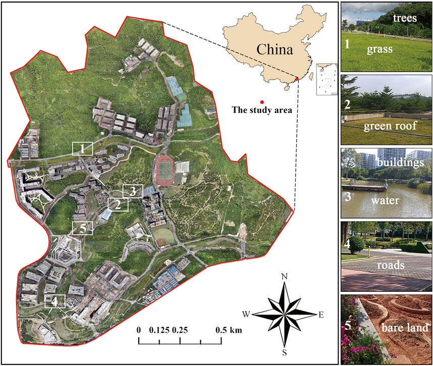
FIGURE 1. The orthophoto map of study area. The numbers 1–5 show the locations of typical infrastructure in the campus, which corresponding pictures are displayed on the right.
There are several types of GI (e.g., green roofs, trees, grass, and bare land), blue infrastructure (e.g., water), and gray infrastructure (e.g., buildings and roads) distributed across the campus (Figure 1). To test the application of UAV images and the method of classifying different types of infrastructure, the SUSTech campus was chosen as the study area.
A DJI Phantom 4 Multispectral (DJI P4M) (DJI, https://www.drdrone.ca/pages/p4-multispectral) UAV was used in this study to obtain the images. The UAV has a built-in stabilizing imaging system, integrating one RGB camera and five multispectral cameras, covering blue (B; 450 ± 16 nm), green (G; 560 ± 16 nm), red (R; 650 ± 16 nm), red-edge (RE; 730 ± 16 nm), and near-infrared (NIR; 840 ± 26 nm), all at two megapixels with a global shutter and on a three-axis gimbal.
Flying missions were performed when the weather conditions were feasible (generally sunny) and the wind was below force 4 (wind speed <6 m/s), at regular intervals of 2–4 weeks. Due to the battery capacity of the UAV, we divided the study area into nine subareas to perform the flying missions. Each mission was carried out between 11:00 and 13:30 in adjacent 2 days and we acquired a total of about 24,600 images from 4,100 photo locations. The UAV can record the precision position information, which could be used for post processed kinematics (PPK) to synthesize the images (https://www.drdrone.ca/pages/p4-multispectral). We used DJI Terra (version 3.0) with orthophoto image correction algorithm to synthesize the images and generate the RGB orthophoto image, the spectral images for the five bands, the digital surface model (DSM), and the normalized difference vegetation index (NDVI) maps (Supplementary Figure S2). The DSM had a resolution of 0.114 m and the other images had a resolution of 0.057 m.
2.2 Classification Algorithms
In this study, six widely used machine learning algorithms were compared. Descriptions, advantages, and disadvantages of the algorithms are shown in Table 1. Detailed explanations and the hyperparameter settings associated with the algorithms are given in Supplementary material S1.
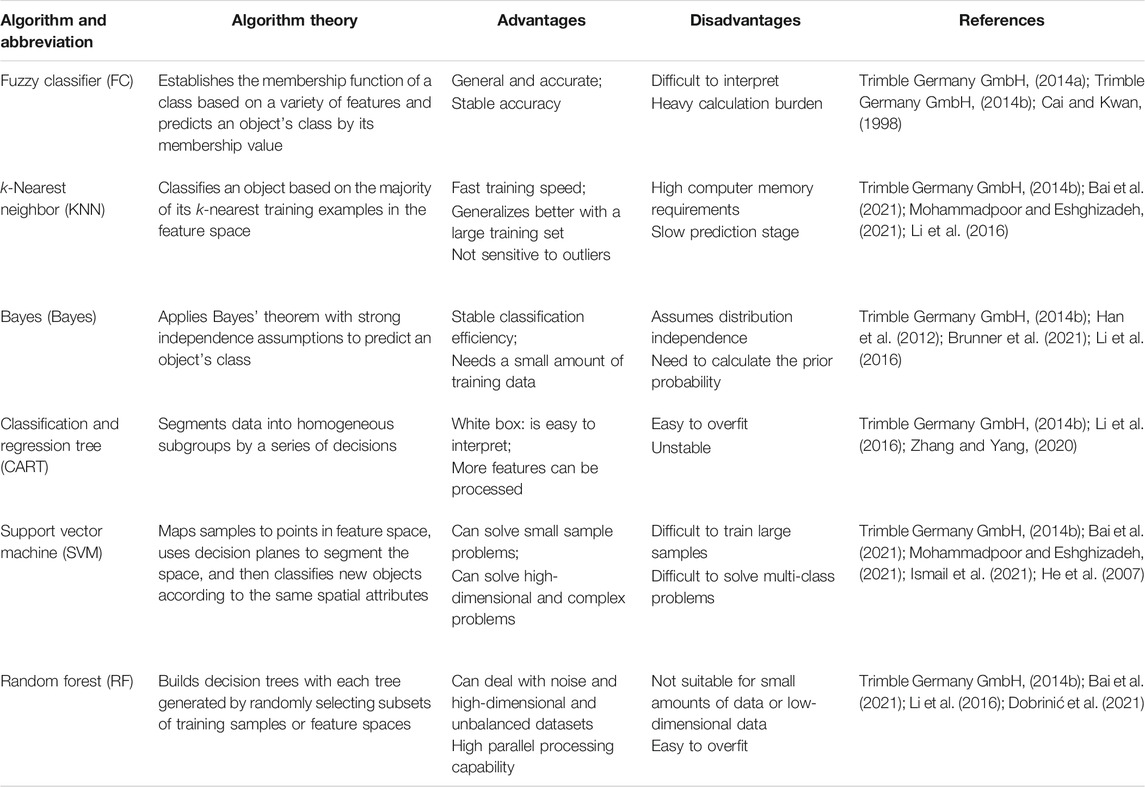
TABLE 1. Six machine learning algorithms adopted in this study.
2.3 Methodology
Figure 2 shows the steps for extracting and classifying the blue-green-gray infrastructure based on the UAV images. Firstly, the input images and RGB orthophoto image were retrieved from the UAV images. Secondly, with the RGB orthophoto image and field survey, we created the training and validation samples for different kinds of infrastructure. Thirdly, based on input images and training samples, we trained the algorithms and got the trained results. Finally, the validation accuracy and classification results were made based on the validation samples and trained results.
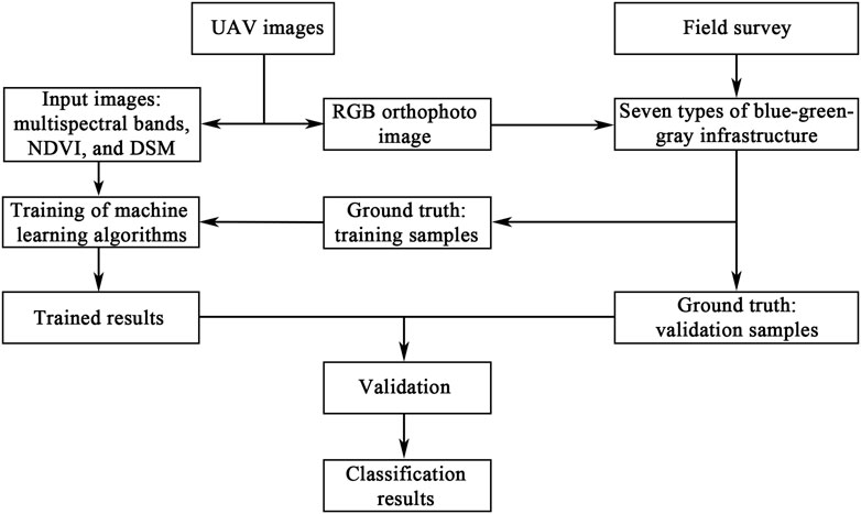
FIGURE 2. Methodology for blue-green-gray infrastructure classification from UAV data.
2.3.1 Sample Creation
Based on the classification categories of the European Commission (Maes et al., 2016), we classified blue-green-gray infrastructure in the SUSTech campus as water, trees (shrubs), grass, green roofs, bare land, buildings (no vegetation), and roads.
The seven types of samples were made for model training and validation of the machine learning algorithms. ArcMap (version 10.6, included in ArcGIS for Desktop, Esri) was used to pre-process input images (Supplementary Figure S2) and make the sample shapefiles for training and validation (Figure 3A). To ensure that the samples were random and the process could be repeated, we applied an equidistant sampling method (chessboard grid sampling method, Figure 3A), which made the samples uniformly distributed (Zhao et al., 2017). To avoid the overlap of samplings, the grids for the validation was obtained by shifting the grids for training, as shown in Figure 3A.
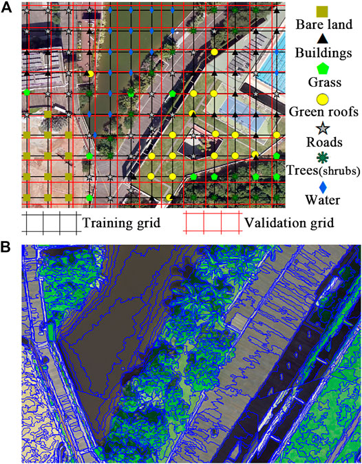
FIGURE 3. (A) Chessboard grid sampling method for making samples. The dots are sample points at the grid intersections. (B) Objects created by multiresolution segmentation, shown as blue polygons.
To achieve a better trade-off between classification accuracy and efficiency, we compared the results derived from samples with different sampling intervals (i.e., 2.9, 5.8, 8.7, 11.6, 14.5, and 17.4 m) in the central part of the campus (referred to as the core area, which is subarea No. 10 in Supplementary Figure S3). The classification accuracies were evaluated at different sampling intervals, and the optimal sampling interval was determined.
2.3.2 Algorithm Training and Validation
Different machine learning algorithms were assessed with Trimble eCognition Developer (eCognition) (version 9.0.2) based on the object-based image analysis method (Trimble Germany GmbH, 2014a). Multiresolution segmentation was used to divide the UAV images into small objects (Figure 3B). The classes were assigned to the objects corresponding to the training samples, and the features of the image layers were extracted to the objects. Each machine learning algorithm was used for training and classification (Figure 4). The accuracy was assessed by the error matrix based on the validation samples and trained results.
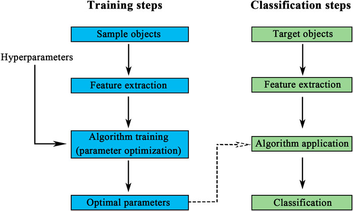
FIGURE 4. Training and classification steps for machine learning algorithms.
We used five widely used indices, producer’s accuracy, user’s accuracy, mean accuracy of different classes, kappa coefficient, and overall accuracy (OA), to evaluate the classification accuracy (Talebi et al., 2014; Dobrinić et al., 2021; Wang et al., 2019; Man et al., 2020). The producer’s accuracy is the ratio of the number of correctly classified objects to validation objects for a class, and the user’s accuracy is the ratio of the number of correctly classified objects to classified objects for a class (Talebi et al., 2014; Dobrinić et al., 2021). The mean accuracy is the average of the producer’s accuracy and user’s accuracy. The kappa coefficient uses information about the entire error matrix to evaluate the classification accuracy and is calculated as (Wang et al., 2019; Man et al., 2020)
where N is the total number of objects, k is the number of classes of the classification, nii is the number of correctly classified objects in class i, ni+ is the objects number classified as class i, and n+i is the number of validation objects of class i.
The OA is the proportion of all sample objects that are correctly classified (Man et al., 2020) and a larger OA value means a better classification result. OA is calculated as (Wang et al., 2019)
The optimal algorithm was obtained by comparing the kappa coefficients and OAs. To test the stability of the best algorithm, we selected the core area and five subareas for accuracy comparison from the total 17 subareas of the study area using a random number generator (Supplementary Figure S3). According to the trial-and-error accuracy assessment, we optimized the selected image layers further by increasing or decreasing the number of layers (see Section 3.6 for details).
3 Results and Discussion
3.1 Optimization of Sampling Method
Our sampling method was first implemented with RF algorithm in the core area, which covered an area of 126,857 m2 and contained seven types of infrastructure. The accuracies of different sampling interval scenarios for various infrastructure types are shown in Table 2. For all infrastructure types, a finer sampling interval corresponded to a higher classification accuracy. A kappa coefficient between 0.80 and 1.00 indicates almost perfect classification, whereas a coefficient between 0.60 and 0.80 indicates substantial classification (Landis and Koch, 1977). The number of samples represents the manual sampling load, and a smaller number indicates higher efficiency. Considering the trade-off between accuracy and sampling efficiency, an optimal sampling interval of 11.6 m was used in this study.
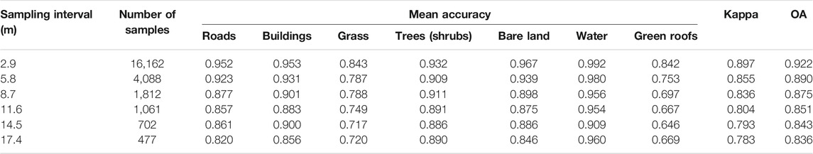
TABLE 2. Accuracy assessment of classification at different sampling intervals.
Common methods for creating sample data include manual selection of the region of interest (Wang et al., 2019), simple random sampling, and equidistant sampling (Zhao et al., 2017). Manual selection is subjective and arbitrary, and thus the results depend on the operator. Simple random sampling is easy to perform, but it may cause polarization and give poor training results (Zhao et al., 2017). The equidistant sampling method, chessboard grid sampling, is objectively random and repeatable. The method produces uniformly distributed samples and mitigates polarization (Zhao et al., 2017), so it can be widely used in other areas. The optimal sampling interval may vary due to the differences in infrastructure type in the target area (e.g., college communities and typical urban areas) and the scale of the infrastructure. Similarly, prioritizing efficiency or accuracy requires different optimal sampling intervals. However, in the areas of the same type (e.g., different college communities), the optimal sampling interval is representative.
3.2 Comparison of Classification Algorithms
Figure 5 shows the classification results of six algorithms in the core area, with a sampling interval of 11.6 m for both training samples and validation samples. The kappa coefficient and OA had the same ranking result, so we took kappa as a representative index for our analysis.
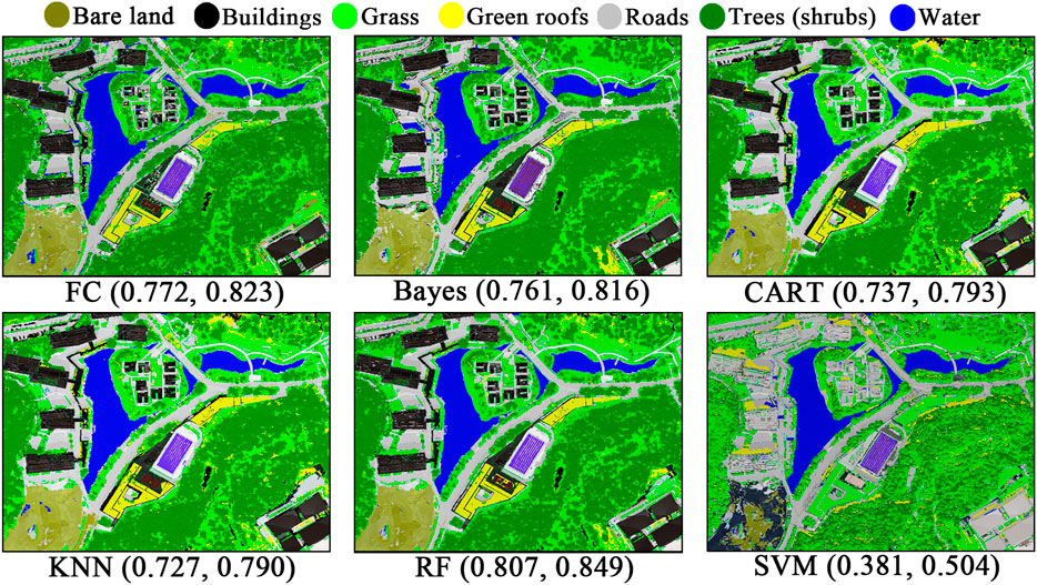
FIGURE 5. Results for the classification algorithms and their kappa coefficients and OAs.
The RF algorithm exhibited the best performance in the core area, with a kappa coefficient of 0.807, demonstrating the advantages of this algorithm in processing high-dimensional data. The following two best classification methods were FC and Bayes, which had similar kappa coefficients of 0.772 and 0.761, respectively. The results calculated with the CART and KNN algorithms showed slightly worse performance. However, the classification results for the SVM algorithm were the worst, with a low kappa coefficient of 0.381. The main reason for this poor performance may be that the SVM algorithm has difficulty in handling large samples and multi-class problems (Bai et al., 2021; He et al., 2007).
3.3 Validation in Other Subareas
The subareas selected for the stability test with RF algorithm were Nos. 3, 5, 13, 14, 17, and 10 (the core area) (Supplementary Figure S3). The classification results, kappa coefficients, and OAs are shown in Figure 6 and Table 3. The kappa coefficients of the five subareas and OAs of the six subareas were greater than 0.8, which reflected an almost perfect performance (Landis and Koch, 1977). The kappa coefficient of subarea No. 3 was 0.592, which was moderate (0.4–0.6) (Landis and Koch, 1977), but the OA was as high as 0.867. This was because the proportion of trees in the training sample set reached about 75% (692/930), which reduced the relative consistency in the calculation (Eq. 1). The mean accuracies of bare land and roads in subarea No. 3 and bare land in subarea No. 13 were below 0.6 (Table 3), which could be associated with the insufficient number of training samples for the related infrastructures. The training samples of them are less than 20. Meanwhile, the classification results were better based on training samples more than 30. From this perspective, to achieve a good result of mapping infrastructure, the training samples should be more than 30.
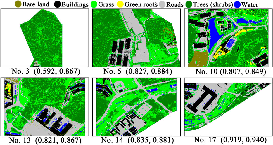
FIGURE 6. Classification results in subareas of the study area, and the kappa coefficients and OAs.
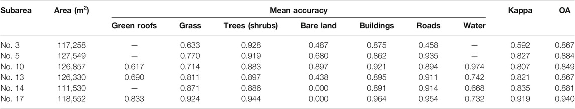
TABLE 3. Classification accuracy assessment in different subareas.
3.4 Effect of Weather Conditions on Classification
In the images taken between August 24, 2020 and December 26, 2020, there were eleven sunny days, three partly cloudy days, and one overcast day. The classification results with RF algorithm were better for the images taken on the overcast day than those taken on the sunny days. We discuss the results from the images taken on December 17, 2020 (overcast) and December 21, 2020 (sunny) as an example. The kappa coefficient and OA for the images taken on the overcast day were greater than those for the sunny day (Table 4). For each type of infrastructure, the mean accuracies of the results derived from the overcast day were higher than those from the sunny day for grass, buildings, and roads. However, for green roofs, better results were obtained from the sunny day.
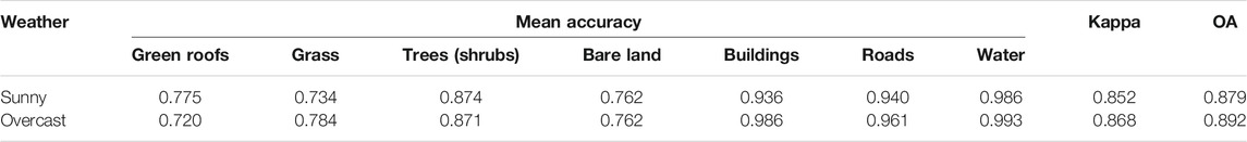
TABLE 4. Comparison of classification accuracy under different weather conditions.
The spectral similarity of grass, trees and green roofs is high (Boonpook et al., 2021). Therefore, we used DSM elevation to increase the difference between green roofs on buildings and vegetation on the ground. Analysis of the locations and image features of the error points (red circles in Figure 7) showed that on a sunny day, the distinction between grass in the shadow of trees and green roofs at the same elevation increased (red circles 6 and 7). In addition, stronger sunlight increased the reflection intensity of leaves on the sunny side of trees (red circles 5 and 6), so the distinction between trees and green roofs also increased. Therefore, accuracy for green roofs was better on the sunny day than on the overcast day. On the sunny day, trees shadows had a strong shading effect on grass (red circle 8), which made it easy to confuse grass with the shaded side of trees. Similarly, shadows of tall buildings blocked out trees and grass (red circles 2 and 3); thus, vegetation in shaded areas could also be misclassified. Therefore, the accuracy of grass was better on the overcast day than on the sunny day. Shadows of tall buildings on the roads were easy to misclassify as water on the sunny day, but not on the overcast day (red circle 1). Under strong Sun on the sunny day, some special coatings on the buildings, such as solar panels, reflected sunlight, which could easily lead to misclassification (red circle 4). On balance, these effects meant that the overcast day image data resulted in better classification results. If the purpose of the flying mission is to obtain spectral data for classification, we recommend doing it on an overcast day with plenty of light.
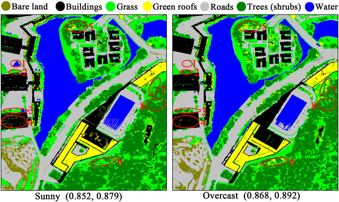
FIGURE 7. Results on a sunny day (left) and an overcast day (right), and the kappa coefficients and OAs. The red circles indicate the main differences between the two subfigures.
3.5 Effect of Seasons on Classification
The kappa coefficients and OAs with RF algorithm in different months of the year (Figure 8) showed that the best classification results were in February (winter) and June (summer), and the kappa coefficient and OA for February were better than those for June.
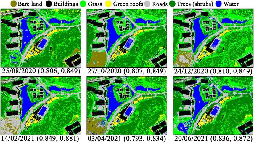
FIGURE 8. Results for different seasons, and the kappa coefficients and OAs.
Table 5 shows that accuracies for grass, roads, and water for February were better than those for June. This may be because the grass was withered or dead in winter, and thus was more easily distinguished from trees on the spectrum. In addition, the tree canopies shrank, so that the increased quantity of light made it easier to identify grass in gaps. As discussed in Section 3.4, shadows made the classification results worse. The area of shadows increases in winter, which could decrease the accuracy. However, grass and trees accounted for a large proportion of the total area, whereas the area of shadows was small, leading to a better classification result in winter. Because the sunlight was weaker in winter, there was a smaller difference between the roads in shadow and the roads in sunlight. Therefore, the mean accuracy of roads was better in winter than in summer. In addition, when the sunlight was close to direct in summer, water surfaces tended to generate mirror reflections, which produced noisy points in the UAV images. Therefore, misclassification of water occurred easily, as shown in the center of the subfigures in Figure 8 (April, June, and August).

TABLE 5. Comparison of classification accuracy for February and June.
Comparing the February and June classification results in Figure 8 and Table 5, the mean accuracy for green roofs in June (i.e., 0.699) was better than that in February (i.e., 0.646). This may be because strong summer sunlight made other vegetation more distinct from the green roofs, which is consistent with the discussion in Section 3.4. Campus construction work caused the change in bare land area that resulted in the difference between the 2 months.
3.6 Effect of Different Image Layers on Classification
The combination of seven image layers (B, G, R, RE, NIR, NDVI, DSM) were used as the benchmark for comparing the results with RF algorithm. By comparing the classification accuracies after reducing the number of image layers, the effects of different layers on the results were analyzed. For convenience, we refer to the results from different layer combinations as cases I–VIII (Figure 9).
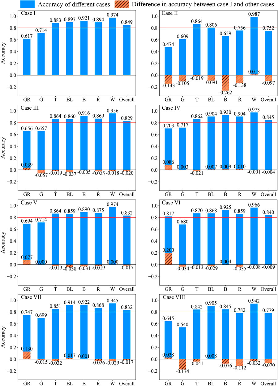
FIGURE 9. Accuracies of classification results with different image layers. The abbreviations for the classes on the abscissa are as follows: GR. green roofs, G. grass, T. trees (shrubs), BL. bare land, B. buildings, R. roads, W. water.
Case I was the benchmark that included all seven layers. Except for green roofs, the mean accuracies in case I were the best. However, the classification result for water was not significantly affected by the different layers, with the accuracies in all the cases larger than 0.94. In most cases, the average accuracies of green roofs and grass were less than 0.8, which indicated that they were easily confused classes.
Case II (B, G, R, RE, NIR, NDVI) did not include the DSM layer. Because green roofs and grass, as well as roads and buildings, have similar features (Boonpook et al., 2021), when the DSM layer was not included, the accuracies of green roofs, grass, buildings, and roads were considerably lower. Therefore, the DSM layer was key information that distinguished green roofs and grass, as well as buildings and roads. To improve the classification accuracy further, the method identifying the four types of infrastructure should be developed in future research. Because green roofs are located on buildings, it may be effective to first extract the buildings, and then identify vegetation on buildings as green roofs. For building recognition, some researchers have used manual extraction (Shao et al., 2021), which is time-consuming and laborious. Due to the different colors and types of building roofs, it is difficult to identify them effectively with only spectral images (Kim et al., 2011). Demir and Baltsavias (2012) and Wang et al. (2018) combined the slope from DSM, spectral images, and other information to identify buildings, and the accuracy was above 0.9. Kim et al. (2011) analyzed LiDAR data to obtain normalized digital surface model (nDSM), and then combined it with airborne images to identify buildings. The nDSM, which is the difference between DSM and digital elevation model, is created from a point cloud (Talebi et al., 2014; Sun and Lin, 2017; Kodors, 2019). Talebi et al. (2014) also used nDSM to distinguish roads, building roofs, and pervious surfaces, and the mean accuracy of building recognition was above 0.8. In summary, using the slope from DSM or nDSM combined with spectral images is effective for identifying buildings, and green roofs, grass, and roads can be accurately classified further.
Case III (B, G, R, RE, NIR, DSM) did not include the NDVI layer. Comparing the results of cases I and III, the accuracies of most classes in case I were higher than those in case III, except for green roofs. The classification subfigures (Supplementary Figure S4) showed that green roofs were overclassified in case I, decreasing the accuracy for green roofs. In case IV (B, G, R, RE, NDVI, DSM), which did not include the NIR layer, the accuracy for green roofs was greatly improved, whereas the OA was still as good as that in case I. The results for case V (B, G, R, NIR, NDVI, DSM), which did not include the RE layer, were similar to those for case IV, but the accuracies for bare land and buildings were lower.
Case VI (B, G, R, NDVI, DSM) did not include the RE and NIR layers, and the accuracy for green roofs was increased substantially by 0.2. The accuracies for grass and roads were decreased, but the other changes were small. The decrease in OA was small, and the classification results were good in general. Case VII (NIR, RE, NDVI, DSM) did not include the B, G, and R bands, and the accuracy for green roofs increased by 0.13. Cases VI and VII showed that appropriate redundancy removal of spectral image layers helped to identify green roofs accurately.
In case VIII (B, G, R, DSM), which did not include the NIR, RE, and NDVI layers, in addition to green roofs and bare land, the accuracies of the other classes were decreased considerably. For overall evaluation, the OA was below 0.8. In particular, the accuracy of grass dropped below 0.6. Case VIII demonstrates the problem of insufficient data layers.
This analysis demonstrated that the DSM layer is crucial for distinguishing green roofs and grass, as well as buildings and roads. Furthermore, appropriate removal of redundant spectral image layers increased the accuracy for green roofs. Case VI (B, G, R, NDVI, DSM) used five image layers, and the green roof accuracy was increased by 0.2 at the cost of decreasing the accuracy for grass by 0.034. The accuracies for the other classes were maintained, which indicated that case VI was the most appropriate combination.
3.7 Limitations
Firstly, although there have been several represented types of infrastructure considered in this study, some other types of green infrastructure (e.g., rain garden) are still missed. Besides, in gray infrastructure, roads can be further subdivided into asphalt roads and porous brick pavements. The porous pavement cannot be recognized in this study. The algorithms and multispectral data used in this paper are capable to recognize the green roofs but not able to distinguish the above finer types effectively.
Secondly, in terms of the sampling method, we only get the optimal sampling interval for college communities. For different types of study areas, we need to conduct trial and error tests to get the optimal sampling interval. This step will still require further improvement.
Thirdly, the remote sensing data we used is limited. If LiDAR point cloud data or DEM data are available, in conjunction with DSM and spectral data, the classification accuracy of green roofs, grass, trees, buildings and roads will be greatly improved.
4 Conclusion
We developed a method to classify blue-green-gray infrastructure accurately using machine learning algorithms and UAV image data. Because the resolution of UAV images is on the centimeter scale, this method could identify all types of infrastructure on a sub-meter scale.
The chessboard grid sampling method was used to ensure the randomness and objectivity of samples. Evaluating the accuracies with different sampling intervals showed that a sampling interval of 11.6 m ensured that the kappa coefficient and OA were in the almost perfect range (>0.8) and that the number of samples was reduced, which increased working efficiency.
There are many machine learning algorithms that can be used for infrastructure classification. The different principles of the algorithms cause differences in their applicability. Evaluating the accuracies of the classification results from six widely used algorithms showed that the RF, FC, and Bayes algorithms were suitable for recognizing different infrastructure. RF was the best algorithm because of its ability to process high-dimensional data well. In addition, the results in other subareas, in which the kappa coefficient and OA were generally greater than 0.8, showed that this method had universal applicability. For any type of infrastructure, more than 30 training samples were needed to ensure the reliability of classification.
Comparing the classification results on a sunny day and an overcast day showed that overcast day data increased the recognition of grass, trees, and roads in shadow. The misclassification of roads in shadow as water was also reduced. The angle of sunlight changes with seasons, which in turn alters the shadow area. In winter, the shadow area is larger, which may reduce the classification accuracy. However, because trees and grass were the main infrastructure types in the study area, shriveled grass in winter increased the spectral difference and classification accuracy. The combination of the two effects resulted in more accurate classification in winter.
To obtain better classification results, we used seven image layers. Through trial and error, we showed that appropriate removal of redundant spectral image layers, such as RE and NIR, increased the recognition accuracy of green roofs. The DSM layer was crucial for improving the distinction considerably between green roofs and grass, and buildings and roads. Using only five image layers (B, G, R, NDVI, and DSM) increased the accuracy for green roofs greatly at the cost of a small decrease in the accuracy for grass.
Our method can identify small facilities on a sub-meter scale, and can obtain a distribution map of blue-green-gray infrastructure in urban small catchments (0.1–10 km2) accurately and quickly. The classification of GI is fundamental for rational management and planning of GI, and contributes to sustainable development of urban areas. Combined with the rainwater use characteristics of various infrastructure, an accurate GI distribution map can help to simulate stormwater management and use effectiveness accurately in small urban catchments.
Data Availability Statement
The raw data supporting the conclusion of this article will be made available by the authors, without undue reservation.
Author Contributions
JJ wrote the manuscript, built the method, acquired data, and conducted data processing and analysis. WC conceived the study, built the method, together wrote this manuscript, and supervised this study. JL conceived the study, acquired funding, supervised the study, and contributed to the manuscript writing.
Funding
This work was supported by the National Key R&D Program of China (2018YFE0206200) and Strategic Priority Research Program of Chinese Academy of Sciences (XDA20060402). It was also supported by the National Natural Science Foundation of China (NSFC) (grant No. 41625001) and the High-level Special Funding of the Southern University of Science and Technology (grant Nos. G02296302 and G02296402).
Conflict of Interest
The authors declare that the research was conducted in the absence of any commercial or financial relationships that could be construed as a potential conflict of interest.
Publisher’s Note
All claims expressed in this article are solely those of the authors and do not necessarily represent those of their affiliated organizations, or those of the publisher, the editors and the reviewers. Any product that may be evaluated in this article, or claim that may be made by its manufacturer, is not guaranteed or endorsed by the publisher.
Acknowledgments
We acknowledge Dr. Wenfang Cao and Pengfei Wang of the iTOWER group for their help with software.
Supplementary Material
The Supplementary Material for this article can be found online at: https://www.frontiersin.org/articles/10.3389/fenvs.2021.778598/full#supplementary-material
References
Alakian, A., and Achard, V. (2020). Classification of Hyperspectral Reflectance Images with Physical and Statistical Criteria. Remote Sensing 12, 2335. doi:10.3390/rs12142335
Bai, Y., Zhang, S., Bhattarai, N., Mallick, K., Liu, Q., Tang, L., et al. (2021). On the Use of Machine Learning Based Ensemble Approaches to Improve Evapotranspiration Estimates from Croplands across a Wide Environmental Gradient. Agric. For. Meteorology 298-299, 108308. doi:10.1016/j.agrformet.2020.108308
Bartesaghi-Koc, C., Osmond, P., and Peters, A. (2020). Quantifying the Seasonal Cooling Capacity of 'green Infrastructure Types' (GITs): An Approach to Assess and Mitigate Surface Urban Heat Island in Sydney, Australia. Landscape Urban Plann. 203, 103893. doi:10.1016/j.landurbplan.2020.103893
Boonpook, W., Tan, Y., and Xu, B. (2021). Deep Learning-Based Multi-Feature Semantic Segmentation in Building Extraction from Images of UAV Photogrammetry. Int. J. Remote Sensing 42, 1–19. doi:10.1080/01431161.2020.1788742
Brunner, M., Von Felten, J., Hinz, M., and Hafner, A. (2021). Central European Early Bronze Age Chronology Revisited: A Bayesian Examination of Large-Scale Radiocarbon Dating. PLOS ONE 15, e0243719. doi:10.1371/journal.pone.0243719
Cui, W., and Chui, T. F. M. (2021). Measurements and Simulations of Energy Fluxes over a High-Rise and Compact Urban Area in Hong Kong. Sci. Total Environ. 765, 142718. doi:10.1016/j.scitotenv.2020.142718
Dai, X., Wang, L., Tao, M., Huang, C., Sun, J., and Wang, S. (2021). Assessing the Ecological Balance between Supply and Demand of Blue-green Infrastructure. J. Environ. Manage. 288, 112454. doi:10.1016/j.jenvman.2021.112454
Demir, N., and Baltsavias, E. (2012). Automated Modeling of 3D Building Roofs Using Image and LiDAR Data. ISPRS Ann. Photogramm. Remote Sens. Spat. Inf. Sci. I-4, 35–40. doi:10.5194/isprsannals-I-4-35-2012
Dimitrov, S., Georgiev, G., Georgieva, M., Gluschkova, M., Chepisheva, V., Mirchev, P., et al. (2018). Integrated Assessment of Urban green Infrastructure Condition in Karlovo Urban Area by In-Situ Observations and Remote Sensing. One Ecosystem 3, e21610. doi:10.3897/oneeco.3.e21610
Dobrinić, D., Gašparović, M., and Medak, D. (2021). Sentinel-1 and 2 Time-Series for Vegetation Mapping Using Random forest Classification: A Case Study of Northern Croatia. Remote Sensing 13 (12), 2321. doi:10.3390/rs13122321
Environmental Protection Agency (2019). Land Cover. United States Environmental Protection Agency. Available at: https://cfpub.epa.gov/roe/indicator.cfm?i=49 (Accessed on November 1, 2021).
Environmental Protection Agency (2015). What Is Green Infrastructure? United States Environmental Protection Agency. Available at: https://www.epa.gov/green-infrastructure/what-green-infrastructure (Accessed on July 12, 2021).
Fan, C., and Lu, R. (2021). UAV Image Crop Classification Based on Deep Learning with Spatial and Spectral Features. IOP Conf. Ser. Earth Environ. Sci. 783, 012080. doi:10.1088/1755-1315/783/1/012080
Furberg, D., Ban, Y., and Mörtberg, U. (2020). Monitoring Urban green Infrastructure Changes and Impact on Habitat Connectivity Using High-Resolution Satellite Data. Remote Sensing 12, 3072. doi:10.3390/RS12183072
Garzon-Lopez, C. X., and Lasso, E. (2020). Species Classification in a Tropical alpine Ecosystem Using UAV-Borne RGB and Hyperspectral Imagery. Drones 4, 69. doi:10.3390/drones4040069
Gašparović, M., and Dobrinić, D. (2021). Green Infrastructure Mapping in Urban Areas Using sentinel-1 Imagery. Croat. J. For. Eng. (Online) 42, 337–356. doi:10.5552/crojfe.2021.859
Gregorio, A. D., and Jansen, L. J. M. (2000). Land Cover Classification System (LCCS): Classification Concepts and User Manual. Food and Agriculture Organization. Available at: https://www.fao.org/3/x0596e/X0596e00.htm (Accessed on November 1, 2021).
Han, J. W., Kamber, M., and Pei, J. (2012). Data Mining: Concepts and Techniques. Beijing: China Machine Press.
Hashad, K., Gu, J., Yang, B., Rong, M., Chen, E., Ma, X., et al. (2021). Designing Roadside green Infrastructure to Mitigate Traffic-Related Air Pollution Using Machine Learning. Sci. Total Environ. 773, 144760. doi:10.1016/j.scitotenv.2020.144760
He, L. M., Shen, Z. Q., Kong, F. S., and Liu, Z. K. (2007). Study on Multi-Source Remote Sensing Images Classification with SVM (In Chinese). J. Image Graphics 4, 648–654. doi:10.3969/j.issn.1006-8961.2007.04.015
Hu, J., Cai, A. Y., Xiao, X. C., Yang, Z. P., Zhou, C., Zhou, W. B., et al. (2008). Feasibility Study Report of Campus Construction Project of South University of Science and Technology (In Chinese). Shenzhen: Shenzhen Quncui Real Estate Appraisal and Construction Consulting Co. Ltd.
Hu, T., Chang, J., and Syrbe, R. U. (2021). Green Infrastructure Planning in Germany and China: a Comparative Approach to green Space Policy and Planning Structure. Res. Urbanism Ser. 6, 99–126. doi:10.7480/rius.6.96
Ismail, A., Juahir, H., Mohamed, S. B., Toriman, M. E., Kassim, A. M., Zain, S. M., et al. (2021). Support Vector Machines for Oil Classification Link with Polyaromatic Hydrocarbon Contamination in the Environment. Water Sci. Techn. 83, 1039–1054. doi:10.2166/wst.2021.038
Jiang, Y., Zhang, L., Yan, M., Qi, J., Fu, T., Fan, S., et al. (2021). High-resolution Mangrove Forests Classification with Machine Learning Using Worldview and UAV Hyperspectral Data. Remote Sensing 13, 1529. doi:10.3390/rs13081529
Khalaim, O., Zabarna, O., Kazantsev, T., Panas, I., and Polishchuk, O. (2021). Urban green Infrastructure Inventory as a Key Prerequisite to Sustainable Cities in Ukraine under Extreme Heat Events. Sustainability 13, 2470. doi:10.3390/su13052470
Kim, Y., Han, Y., Byun, Y., Choi, J., Han, D., and Kim, Y. (2011). “Object-based Classification of an Urban Area through a Combination of Aerial Image and Airborne Lidar Data,” in American Society for Photogrammetry and Remote Sensing Annual Conference 2011, 265–270. Available at: https://www.scopus.com/inward/record.uri?eid=2-s2.0-84868623294&partnerID=40&md5=67b8f95b588f1f61c8865bc09fd897b6.
Kodors, S. (2019). Comparison of Algorithms for Construction Detection Using Airborne Laser Scanning and nDSM Classification. Environ. Techn. Resour. Proc. Int. Scientific Pract. Conf. 2, 79–83. doi:10.17770/etr2019vol2.4032
Landis, J. R., and Koch, G. G. (1977). The Measurement of Observer Agreement for Categorical Data. Biometrics 33, 159–174. doi:10.2307/2529310
Li, M., Ma, L., Blaschke, T., Cheng, L., and Tiede, D. (2016). A Systematic Comparison of Different Object-Based Classification Techniques Using High Spatial Resolution Imagery in Agricultural Environments. Int. J. Appl. Earth Observation Geoinformation 49, 87–98. doi:10.1016/j.jag.2016.01.011
Lynn Yaling Cai, L. Y., and Hon Keung Kwan, H. K. (1998). Fuzzy Classifications Using Fuzzy Inference Networks. IEEE Trans. Syst. Man. Cybern. B 28, 334–347. doi:10.1109/3477.678627
Machine Learning (2018). A Step by Step CART Decision Tree Example. Sefik Ilkin Serengil. Available at: https://sefiks.com/2018/08/27/a-step-by-step-cart-decision-tree-example/(Accessed on July 12, 2021).
Maes, J., Zulian, G., Thijssen, M., Castell, C., Baro, F., Ferreira, A., et al. (2016). Mapping and Assessment of Ecosystems and Their Services: Urban Ecosystems 4th Report. Luxembourg: Publication Office of the European Union. JRC101639. doi:10.2779/625242
Man, Q., Dong, P., Yang, X., Wu, Q., and Han, R. (2020). Automatic Extraction of Grasses and Individual Trees in Urban Areas Based on Airborne Hyperspectral and LiDAR Data. Remote Sensing 12, 2725. doi:10.3390/RS12172725
Meteorological Bureau of Shenzhen Municipality (2021). Climate Situation and Characteristics of Seasons in Shenzhen. Meteorological Bureau of Shenzhen Municipality. Available at: http://weather.sz.gov.cn/qixiangfuwu/qihoufuwu/qihouguanceyupinggu/qihougaikuang/(accessed on July 12, 2021).
Miura, N., Koyanagi, T. F., Yamada, S., and Yokota, S. (2021). Classification of Grass and Forb Species on Riverdike Using UAV LiDAR-Based Structural Indices. Int. J. Automation Technol. 15, 268–273. doi:10.20965/ijat.2021.p0268
Mohammadpoor, M., and Eshghizadeh, M. (2021). Introducing an Intelligent Algorithm for Extraction of Sand Dunes from Landsat Satellite Imagery in Terrestrial and Coastal Environments. J. Coast Conserv 25, 3. doi:10.1007/s11852-020-00789-x
Narziev, J., Nikam, B., and Gapparov, F. (2021). Infrastructure Mapping and Performance Assessment of Irrigation System Using GIS and Remote Sensing. E3s Web Conf. 264, 03005. doi:10.1051/e3sconf/202126403005
Nitoslawski, S. A., Wong-Stevens, K., Steenberg, J. W. N., Witherspoon, K., Nesbitt, L., and Konijnendijk van den Bosch, C. C. (2021). The Digital Forest: Mapping a Decade of Knowledge on Technological Applications for Forest Ecosystems. Earth's Future 9 (8), e2021EF002123. doi:10.1029/2021EF002123
Ouyang, W., Morakinyo, T. E., Ren, C., Liu, S., and Ng, E. (2021). Thermal-irradiant Performance of green Infrastructure Typologies: Field Measurement Study in a Subtropical Climate City. Sci. Total Environ. 764, 144635. doi:10.1016/j.scitotenv.2020.144635
Palmer, M. A., Liu, J., Matthews, J. H., Mumba, M., and D'Odorico, P. (2015). Manage Water in a green Way. Science 349 (6248), 584–585. doi:10.1126/science.aac7778
Shao, H., Song, P., Mu, B., Tian, G., Chen, Q., He, R., et al. (2021). Assessing City-Scale green Roof Development Potential Using Unmanned Aerial Vehicle (UAV) Imagery. Urban For. Urban Green. 57, 126954. doi:10.1016/j.ufug.2020.126954
Sudarshan Rao, B., Hota, M., and Kumar, U. (2021). Crop Classification from UAV-Based Multi-Spectral Images Using Deep Learning. Comm. Com. Inf. Sc. 1376, 475–486. doi:10.1007/978-981-16-1086-8_42
Sun, X. F., and Lin, X. G. (2017). Random-forest-ensemble-based Classification of High-Resolution Remote Sensing Images and nDSM over Urban Areas. Int. Arch. Photogramm. Remote Sens. Spat. Inf. Sci. XLII-2/W7, 887–892. doi:10.5194/isprs-archives-XLII-2-W7-887-2017
Talebi, L., Kuczynski, A., Graettinger, A. J., and Pitt, R. (2014). Automated Classification of Urban Areas for Storm Water Management Using Aerial Photography and LiDAR. J. Hydrol. Eng. 19, 887–895. doi:10.1061/(ASCE)HE.1943-5584.0000815
Trimble Germany GmbH, (2014a). eCognition Developer 9.0 Reference Book. Munich: Trimble Germany GmbH.
Venkataramanan, V., Packman, A. I., Peters, D. R., Lopez, D., McCuskey, D. J., McDonald, R. I., et al. (2019). A Systematic Review of the Human Health and Social Well-Being Outcomes of green Infrastructure for Stormwater and Flood Management. J. Environ. Manage. 246, 868–880. doi:10.1016/j.jenvman.2019.05.028
Wang, H., Han, D., Mu, Y., Jiang, L., Yao, X., Bai, Y., et al. (2019). Landscape-level Vegetation Classification and Fractional Woody and Herbaceous Vegetation Cover Estimation over the Dryland Ecosystems by Unmanned Aerial Vehicle Platform. Agric. For. Meteorology 278, 107665. doi:10.1016/j.agrformet.2019.107665
Wang, J. B., Jin, Q., Yang, G. D., Zhang, X. Q., Zhan, G. Q., and Shao, P. (2018). A Building Extraction Method Based on Object-Oriented Technology and DSM Image (In Chinese). Glob. Geology. 37, 1258–1264. doi:10.3969/j.issn.1004-5589.2018.04.026
Wicaksono, A., and Hernina, R. (2021). Urban Tree Analysis Using Unmanned Aerial Vehicle (UAV) Images and Object-Based Classification (Case Study: University of Indonesia Campus). IOP Conf. Ser. Earth Environ. Sci. 683, 012105. doi:10.1088/1755-1315/683/1/012105
Yang, Y., Li, J., Huang, Q., Xia, J., Li, J., Liu, D., et al. (2021). Performance Assessment of Sponge City Infrastructure on Stormwater Outflows Using Isochrone and SWMM Models. J. Hydrol. 597, 126151. doi:10.1016/j.jhydrol.2021.126151
Zhang, F., and Yang, X. (2020). Improving Land Cover Classification in an Urbanized Coastal Area by Random Forests: The Role of Variable Selection. Remote Sensing Environ. 251, 112105. doi:10.1016/j.rse.2020.112105
Zhang, J., Feng, X., Shi, W., Cui, J., Peng, J., Lei, L., et al. (2021). Health Promoting green Infrastructure Associated with green Space Visitation. Urban For. Urban Green. 64, 127237. doi:10.1016/j.ufug.2021.127237
Keywords: green infrastructure, blue infrastructure, classification, unmanned aerial vehicle images, machine learning
Citation: Jia J, Cui W and Liu J (2022) Urban Catchment-Scale Blue-Green-Gray Infrastructure Classification with Unmanned Aerial Vehicle Images and Machine Learning Algorithms. Front. Environ. Sci. 9:778598. doi: 10.3389/fenvs.2021.778598
Received: 17 September 2021; Accepted: 22 December 2021;
Published: 17 January 2022.
Edited by:
Laixiang Sun, University of Maryland, United StatesCopyright © 2022 Jia, Cui and Liu. This is an open-access article distributed under the terms of the Creative Commons Attribution License (CC BY). The use, distribution or reproduction in other forums is permitted, provided the original author(s) and the copyright owner(s) are credited and that the original publication in this journal is cited, in accordance with accepted academic practice. No use, distribution or reproduction is permitted which does not comply with these terms.
*Correspondence: Junguo Liu, anVuZ3VvLmxpdUBnbWFpbC5jb20=, bGl1amdAc3VzdGVjaC5lZHUuY24=
†These authors have contributed equally to this work and share first authorship