Hybrid Data Mining Forecasting System Based on Multi-Objective Optimization and Selection Model for Air pollutants

The air quality index (AQI) indicates the short-term air quality situation and changing trend of the city, which includes six air pollutants: PM_2.5, PM₁₀, CO, NO₂, SO₂ and O₃. Due to the diversity of pollutants and the fluctuation of single pollutant time series, it is a challenging task to find out the main pollutants and establish an accurate forecasting system in a city. Previous studies primarily focused on enhancing either forecasting accuracy or stability and failed to analyze different air pollutants at length, leading to unsatisfactory results. In this study, a model selection forecasting system is proposed that consists of data mining, data analysis, model selection, and multi-objective optimized modules and effectively solves the problems of air pollutants monitoring. The proposed system employed fuzzy C-means cluster algorithm to analyze 13 original AQI series, and fuzzy comprehensive evaluation is used to find out the main air pollutants in each city. And then multiple artificial neural networks are used to forecast the main air pollutants for each category and find the optimal models. Finally, the modified multi-objective optimization algorithm is used to optimize the parameters of optimal models and model selection to obtain final forecasting values from optimal hybrid models. The experiment results of datasets from 13 cities in the Beijing–Tianjin–Hebei Urban Agglomeration demonstrated that the proposed system can simultaneously obtain efficient and reliable data for air quality monitoring.

Introduction

In recent years, air pollution has received increasing attention due to the negative effects, such as respiratory diseases, that it has on human health (Jiang et al., 2017). Simultaneously, air pollution is a growing environmental concern, responsible for approximately 2 million premature deaths per year worldwide (World Health Organization, 2008). A report issued by the World Health Organization (WHO) acknowledges that air pollution is one of the biggest health risks (Xu et al., 2016). Since the industrial revolution, many countries have focused on economic development while ignoring air quality, and incidents that cause harm are everywhere. In 1930, the Mas Valley event in Belgium caused nearly 60 deaths in a week. In the 1940s, the smog incident in Los Angeles caused many people to have red eyes, pharyngitis, respiratory disease deterioration, and even confusion and pulmonary edema. In 1948, the American Donora incident caused 5,911 people to become violent. The most serious is the well-known London smog event of 1952—more than 4,000 deaths in 4 days and more than 8,000 deaths in 2 months. In addition, air pollution in China is also quite serious. The previous results in 2009 showed that the air quality index (AQI) in 107 cities of China did not meet the country's national air quality standards (NAAS) (Zhou et al., 2014). In addition, 7 of the 10 most polluted cities in the world are in China. According to the World Bank, China loses 10% of its gross domestic product each year due to air pollution. Air pollution is also associated with elevated rates of mortality, causing between 350,000 and 500,000 premature deaths each year in China (Shanshan et al., 2014). Air pollution has become the fourth leading health risk factor for China after smoking, diet, and obesity (Zhang et al., 2018). In order to reduce the losses caused by air pollution, several health and governmental institutions gather and publish data regarding what is known as AQI to inform people about the state of air pollution. For instance, the European Environment Agency (EEA) and the European Commission (EC) have launched, in 2017, an online platform that provides information about current air quality situation based on measurements from more than 2,000 air quality monitoring stations across Europe (Akyüz and Çabuk, 2009). In addition, China's environmental supervisors have also issued some plans and programs, including EIA (Environmental Influence Assessment) and Emergency Response for reducing air pollution. Since 2013, China has also begun to evaluate the quality of air through AQI values and graded the city's air quality by AQI values. AQI is an important evaluation indicator that comprehensively reflects the air pollution status related to human health. Through the use of the AQI it was possible to synthesize, in a single daily value, concentrations of major pollutants in urban areas (NO₂, O₃, CO, SO₂, PM_2.5, PM₁₀) for the entire period (Feng et al., 2015). The greater the AQI value, the more serious the air pollution. But real-time air quality monitoring can no longer meet people's needs. Like weather forecasts, people also long for air quality prediction to arrange their activities and take protective measures in advance (Hao et al., 2021).

Obviously, if we can provide early warning before the hazard occurs, based on a good air quality early-warning system, these losses might be avoided by taking effective corresponding protection measures. In order to establish an effective air warning system, observation and control of air quality is the key issue for authorities. The most significant point in any kind of air pollution control system is to be able to detect increasing (deterioration) or decreasing (improvement) trends (Hao and Tian, 2018). Unfortunately, because air quality data is obtained in limited time and space, its incompleteness and non-stationarity may result in low accuracy and poor stability of the forecasting results (Hao et al., 2019). Therefore, the prediction of AQI or other pollution indicators is a challenging task.

In recent years, many studies on air quality have focused on the prediction of atmospheric pollutant concentrations. From the angle of methodology, various quantitative prediction methods of the atmosphere pollutant concentrations can be classified into two categories, including deterministic models and empirical models (Steffens et al., 2017). The deterministic model is mainly the chemical transport model (CTM), which is based on the fundamental principles of simulating atmospheric physics and chemistry that involve transportation, emissions, and conversion processes in air pollution (Rivas et al., 2018). The forecasts are used to support flight planning by enabling the representation of important three-dimensional (3-D) atmospheric chemical structures (such as dust storm plumes, polluted air masses originated by large cities, and widespread biomass burning events) and their time evolution, which are often research targets to be detected and investigated through specific flight plans (Latif et al., 2018). Various models have been proposed to identify the interactions between various air pollutants and their emission sources (Yang and Wang, 2017). Nonetheless, due to the incomplete knowledge and understanding of the sources, dispersion and sinks of pollutants, transport processes, and atmospheric chemicals, there are some significant uncertainties in the models, resulting in air pollutant concentrations being among the most difficult to forecast accurately using CTMs (Liu et al., 2008). Therefore, CTM forecasts are less accurate than empirical air quality predictive models that are trained with local meteorological data and air quality.

A large number of empirical models include statistical models and machine learning models for the forecast of atmospheric pollutant concentrations. Common statistical models for air quality prediction include autoregressive (AR) models, moving average (MA) models, autoregressive integrated moving average (ARIMA) models, and multiple linear regression (MLR) models. For example, Zhang et al. (2018) applied the RIMA model to predict the concentration of PM_2.5 based on time series air quality data covering two warm periods and two cold periods and concludes that PM_2.5 concentration is higher in the cold period and lower in the warm period. MLR models are applied by Mehmet Akyüz et al. (Pereira et al., 2018) to forecast the concentration of individual pollutants. The study also considers the effects of contaminant concentrations and other meteorological parameters. Although Box–Jenkins Time Series (ARIMA) and MLR models have been applied to air quality forecasting in urban areas, they have limited accuracy owing to their inability to predict extreme events, and they are not applicable when performing long-term prediction and nonlinear sequence prediction.

On the contrary, artificial neural networks (ANNs) are more popular for their no-linear systems, especially when it is difficult to determine the theoretical models (Lanzafame et al., 2015). Díaz-Robles et al. (2008) combined a new hybrid model of ARIMA and ANN to improve the prediction accuracy of areas with limited air quality and meteorological data. Xiao Feng and Qi Li et al. (Feng et al., 2015) combined air mass trajectory analysis and wavelet transform and proposed that ANN predicts the daily average concentration of pollutants 2 days in advance, improves the accuracy of prediction, and is superior to other models. However, they also have certain shortcomings that may fall into local optimum or over-fitting, which may result in poor prediction.

Any model has its inevitable shortcomings, and due to the advent of the world's big data era, data mining techniques such as decomposition methods (Güçlü et al., 2019), feature selection techniques (Pan et al., 2011), and optimization algorithms (Liu et al., 2019) combined with artificial intelligence technology are more operational. Therefore, with consideration of forecast accuracy, hybrid models which combine a new method with artificial intelligence are of great significance in air quality forecasting field (D'Allura et al., 2011). Although the construction of the combined model is usually based on actual problems to achieve the expected test objectives, there are still some problems that most of the past studies have focused on improving the prediction accuracy of the model while ignoring the stability of the model prediction. Many optimization algorithms inspired by nature including cuckoo algorithm (Urbancok et al., 2017), firefly algorithm (Bessagnet et al., 2019), bat algorithm (Liu et al., 2018), and particle swarm optimization algorithm (Kumar et al., 2019) have been developed to solve single-objective problems in recent years. However, real-world optimization problems always involve multiple objectives and so-called multi-objective optimization, which means, in this case, the solutions for a multi-objective problem, which is the main focus of the algorithm, represent the trade-offs between the objectives due to the nature of such problems (Shenfield and Rostami, 2015). The developed multi-objective optimization algorithm has been applied more and more widely in the fields of finance (Li et al., 2019) and mechanical engineering (Dhiman and Kumar, 2018). The atmosphere is a highly complex dynamic system. The air quality data sequence usually has characteristics such as non-stationarity and nonlinearity; thus, the multi-objective optimization algorithm is a suitable choice.

Furthermore, air quality assessment algorithms are developed to assess air quality and protect human health from air pollution and play a vital role in air quality warning systems. The early-warning system can increase the environmental consciousness of society and protect the public against hazardous air quality. It can also aid the relevant departments to better control air pollution and avoid negative social, economic, and environmental impacts. According to the aforementioned analysis, developing a novel and robust air quality early-warning system has become highly desirable for society. Therefore, a variety of models are employed in air quality assessment, including mobile monitoring (Li et al., 2018), CFD-RANS simulation (Lauriks et al., 2020), principal component regression (PCR), sensitivity analysis (Kim et al., 2018), Bayesian models (Han et al., 2021), support vector machines (SVM) (Leong et al., 2019), ANNs (Davood et al., 2021), and fuzzy techniques (Dass et al., 2021). However, although the air quality warning system has important practical significance to the public in other fields, China's research in this field is still relatively small.

Looking back at the previous literature on air quality forecasting research, the shortcomings of the traditional air quality forecasting models are summarized as follows: 1) the large amount of information required by the CTM model leads to uncertainty in the forecasting. 2) The single statistical models with low forecasting accuracy cannot meet the requirements of air quality forecasting. 3) In the past, many air quality studies focused on eliminating the effects of noise on data processing and less on the feature extraction of data. 4) It is easy for single-objective optimization algorithm commonly used to fall into local optimum and over-fitting, resulting in poor stability. 5) In addition, previous studies on air quality have focused on air quality forecasting, while the research on air quality assessment was relatively rare.

Based on the above analysis, it is necessary to overcome these deficiencies and develop a novel and robust air quality warning system. The evaluation–forecast system developed in this study consists of two parts: evaluation and forecasting. The evaluation part involves feature extraction and finding out the main air pollutants; in the forecasting part, a new metric is developed to find the optimal model in each category, and optimal forecasting models are optimized with modified gray wolf optimization (DEGWO) optimization algorithm and leave-one-out deciding weight strategy to improve the accuracy of forecasting results and provide support for early warning systems. The specific implementation steps of the hybrid forecasting system are as follows: First, the feature extraction of the original data is performed to find similar attributes of AQI time series according to the relevant theory of fuzzy C-mean cluster.

Moreover, air quality evaluation based on the forecasting results of air pollutant concentration plays a crucial role in the development of the air quality warning system.

In this paper, in view of the uncertainty and ambiguity of each air pollutant, the fuzzy comprehensive evaluation is applied in AQI. According to the implementation of fuzzy comprehensive evaluation results, finding out the main pollutants in each city is another important part of this work. Next, we use long short-term memory (LSTM), backpropagation neural network (BPNN), adaptive network-based fuzzy inference system (ANFIS), generalized regression neural network (GRNN), and SVM models to forecast the main air pollutants time series, and a developed new metric is used to select optimal forecasting model. Finally, all these individual forecasting models' predictors based on the leave-one-out deciding weight strategy are optimized by the DEGWO optimization algorithm, and the final forecasting results are obtained. Therefore, the combination of these methods will result in more accurate forecasts and assessments performance, providing significant advantages for the construction and implementation of early warning systems for detecting air quality. The main contributions of this paper are as follows:

1) The fuzzy comprehensive evaluation is established for six air pollutants, which calculates the fuzzy membership degree of each pollutant and determines the main pollutants of each city.

2) A model selection index is established to select the optimal forecasting model from different neural network models. Based on model selection, the established weighted information criterion can select the optimal forecasting model for PM_2.5, PM₁₀, and NO₂ forecasting.

3) The forecasting performance of the optimal single model is improved. In the forecasting process, an improved multi-objective optimization algorithm is used to optimize the parameters of the single forecasting model, which not only improves the prediction accuracy but also improves the stability of the single model

4) The model selection index is used to select the optimal forecasting value from the optimal hybrid model.

Methodology

In this subsection, the relative methods are presented in detail, including the data mining technique, forecasting model, and the DEGWO) algorithm. Subsequently, the marching process of our developed combined model is demonstrated.

Forecasting Model

Five typical models, namely, the multilayer perceptron (MLP) (You et al., 2017), ANFIS (Jang, 1993), LSTM (Muzaffar and Afshari, 2019), SVM (Brereton and Lloyd, 2010), and GRNN (Land and Schaffer, 2020), have been widely used for air pollutants forecasting because of their robustness, efficiency, and accuracy.

Modified Gray Wolf Optimization (DE-GWO)

For the DE algorithm and gray wolf optimization (GWO) algorithm, the defects of prematurity, poor stability, and ease in falling into local optimum will occur when solving the optimization problem separately. Combining the advantages and disadvantages of the two algorithms, a more efficient hybrid optimization algorithm, DEGWO algorithm, is proposed to improve global search capabilities.

Firstly, in order to avoid the phenomenon in which the population is iteratively reduced to a certain area, the crossover and selection operations of the DE algorithm are used to maintain the diversity of the population. Then, as the initial population of the GWO algorithm, the objective function value of the individual is calculated. The optimal three individuals X_α, X_β, and X_δ are selected to update the positions of other gray wolf individuals. Then, the position of the gray wolf individual is updated by the intersection and selection operations of DE, and the iterative update is repeated until the optimal one is selected. The target function value is output.

The hybrid algorithm not only improves the global search ability but also effectively avoids the defects of early maturity stagnation and falling into local optimum. The specific implementation steps of the algorithm are as follows:

Step 1: Set the relevant parameters of the hybrid optimization algorithm, population size N, maximum iteration number t_max, crossover probability CR, search dimension D, search range ub, lb, and scaling factor range F.

Step 2: The parameters a, A, and C are initialized, and the DE variant operation is performed on the population individual according to Eq. 1 to generate an intermediate; an initial population and the number of iterations is set to t = 1.

$v_{ij}\left(g+1\right)=\{\begin{array}{c}{h}_{ij}\left(g\right), rand\left(\mathrm{0,1}\right)\le \begin{array}{ccc}CR& or& j=rand\left(1,n\right)\end{array}\\ x_{ij}\left(g\right), rand\left(\mathrm{0,1}\right)>\begin{array}{ccc}CR& or& j\ne rand\left(1,n\right)\end{array}\end{array}(1)$

Then the competition selection operation is performed according to Eq. 2 to generate.

$x_i\left(g+1\right)=\{\begin{array}{c}{v}_i\left(g\right), f\left[v_i\left(g+1\right)\right] <f\left[x_i\left(g+1\right)\right] \\ x_i\left(g\right), f\left[v_i\left(g+1\right)\right] \ge f\left[x_i\left(g+1\right)\right]\end{array}(2)$

Step 3: Calculate the objective function value of each gray wolf individual in the population, sort according to the size of the objective function value, and select the optimal first three individuals as X_α, X_β, and X_δ, respectively.

Step 4: Calculate the distance between other gray wolf individuals in the population and the optimal X_α, X_β, and X_δ according to Eqs 3–5.

$D_{\alpha }=\left|C_1{X}_{\alpha }\left(t\right)-X\left(t\right)\right|(3)$

$D_{\beta }=\left|C_2{X}_{\beta }\left(t\right)-X\left(t\right)\right|(4)$

$D_{\delta }=\left|C_3{X}_{\delta }\left(t\right)-X\left(t\right)\right|(5)$

Finally, update the current position of each gray wolf individual according to Eqs 6–9.

$X_1\left(t+1\right)=X_{\alpha }\left(t\right)-A_1{D}_{\alpha }(6)$

$X_2\left(t+1\right)=X_{\beta }\left(t\right)-A_2{D}_{\beta }(7)$

$X_3\left(t+1\right)=X_{\delta }\left(t\right)-A_3{D}_{\delta }(8)$

$X_p\left(t+1\right)=\frac{X_1+X_2+X_3}{3}(9)$

Step 5: Update the values of a, A, and C in the algorithm, cross-operate the position of the individual population according to Eq. 1, retain the better components, then perform Eq. 2 to select new individuals and calculate the objective function values of all gray wolf individuals.

Step 6: Update the positions of the top three gray wolf individuals X_α, X_β, and X_δ.

Step 7: Determine the count value. If the maximum iteration number t_max is reached, the algorithm exits and, based on Eq. 10, outputs the multi-objective function value of the global optimal X_α; otherwise, let t = t + 1, and then go to Step 3 to continue execution.

$\min f=f_1\left(x\right)+f_2\left(x\right)$

$s.t\{\begin{array}{c}{f}_1\left(x\right)=\frac{1}{n}{\displaystyle \sum _{i=1}^n{\left(erro{r}_i\right)}^2}\\ f_2\left(x\right)=\frac{1}{n}{\displaystyle \sum _{i=1}^n{\left(erro{r}_i-\overline{error}\right)}^2}\end{array}(10)$

Fuzzy C-Means Clustering

Fuzzy C-means clustering (FCM), known as fuzzy ISODATA, is a clustering algorithm that uses membership degrees to determine the extent to which each data point belongs to a certain cluster. In 1973, Bezdek proposed the algorithm as an improvement to the early hard C-means clustering (HCM) method (Gayen and Biswas, 2021). The clustering steps are as follows:

Step 1: Initialize the membership matrix U with a random number whose value is between 0 and 1, so that it satisfies the constraint in Eq. 11.

${\displaystyle \sum _{i=1}^c{u}_{ij}}=1,{\forall }_j=1,\mathrm{...},n(11)$

Step 2: Calculate c cluster centers c_i (i = 1, c) using Eq. 12.

$c_i=\frac{{\displaystyle \sum _{j=1}^n{u}_{ij}^m{x}_j}}{{\displaystyle \sum _{j=1}^n{u}_{ij}^m}}(12)$

Step 3: Calculate the value function according to Eq. 13. If it is less than a certain threshold, or if the amount of change from the value of the last value function is less than a certain threshold, the algorithm stops.

$\text{J}\left(\text{U}{c}_1\text{,}\mathrm{...}\text{,}{c}_c\right)={\displaystyle \sum _{\text{i}=1}^{\text{c}}{J}_i={\displaystyle \sum _{i=1}^c{\displaystyle \sum _j^n{u}_{ij}^m{d}_{ij}^2}}}(13)$

Step 4: Calculate the new U matrix with Eq. 14. Go back to Step 2.

$u_{ij}=\frac{1}{{\displaystyle \sum _{k=1}^c{\left(\frac{d_{ij}}{d_{kj}}\right)}^{\frac{2}{\left(m-1\right)}}}}(14)$

Fuzzy Synthetic Evaluation Theory

The process of establishing a fuzzy synthetic evaluation (FSE) system is as follows (Lu et al., 2011).

Step 1. The set of factors for the evaluation object is determined.

The selected factors should possess the traits of representativeness, feasibility, and system. Air quality evaluation relies on the concentration levels of the main air pollutants. Therefore, in this study, the indicators were chosen according to China's ambient air quality standards (AAQS: GB3095-2012). Moreover, different geographical areas have different topographic and economic characteristics, and consequently, the different key pollutants in the study areas should be also considered.

Step 2. The evaluation rank standard is determined.

The evaluation rank set is described as V = {v₁, v₂,$\cdots$,v_n}. In our study, the air pollution degrees were divided into five levels. The pollutants grading standard according to AAQS is shown in Supplementary Appendix S1.

Step 3. Index fuzzification.

In this step, the membership functions (MFs) corresponding to each index are obtained. The process of fuzzification constitutes the process of membership calculation by using MFs. In this study, we used the trapezoidal membership to calculate the membership value.

Step 4. The factor weight is calculated.

Weight reflects the importance of each factor in synthetic evaluation and directly affects the outcome of the evaluation. Many methods exist for determining the weight, such as weighted statistics, coefficient of variation method, the Delphi method, and entropy methods. In our study, the weight was calculated by fuzzy weighting method.

Step 5. The evaluation results are output.

The objective function of the DEGWO algorithm is based on stability and accuracy, in which MSE is the standard to measure accuracy and the variance of error is the standard to measure stability. Algorithm 1 briefly outlines the process of the MODEGWO.

Algorithm 1 MMODAInput: Objective function Min fitness(x) = f₁ + f₂

$min\{\begin{array}{l}{f}_1\left(x\right)=MSE=\frac{1}{\mathit{N}}{\displaystyle \sum _{i=1}^N({\widehat{x}}_i-x_i),i=\mathrm{1,2},\mathrm{...},N}\\ f_2\left(E\right)=Var\left(E\right)=\frac{1}{N}{\displaystyle \sum _{i=1}^N{(E_i-\overline{E})}^2},i=\mathrm{1,2},\mathrm{...},N\end{array}$

Note: $E_i$ is the test error; the calculation equation is $E_i={\widehat{x}}_i-x_i$

 ${\widehat{x}}_i$ and $x_i$ are the actual data and output data by each model

  Parameters of DEGWO

  CR is crossover probability: 0.2;

  MaxGen is the maximum number of the iteration: 500;

  F is the scaling factor: [0.2, 0.8];

  p_size is population size: 50.

Output: The optimal solution and the best objective function value.

Initialize a parent population, mutant population, and child population of gray wolf with a random position in a feasible region using equation;

$x_p^k=x_p^k\left(low\right)+(x_p^k\left(up\right)-x_p^k\left(low\right))\times rand\left(\mathrm{0,1}\right)$

Note: $x_p^k\left(low\right)$is the lower bound of the pth component of the kth individual.

 $x_p^k\left(up\right)$ is the upper bound of the pth component of the kth individual.

 rand(0, 1) represents a random number in [0, 1].

 p = 1, 2$\cdots$, d. k = 1, 2$\cdots$, p_size

Initialize crossover probability Pc and scaling factor F;

Initialize a, A, and C;

Evaluate f for all individuals in the parent population;

Sort the parent population in a non-decreasing order, according to the objective function value;

X_α is the best individual in the parent population of gray wolves;

X_β is the second individual in the parent population of gray wolves;

X_δ is the third individual in the parent population of gray wolves;

While (t < MaxGen)

for each individual in the parent population of gray wolves

Update the position using the following equation;

$X_p(t+1)=\frac{X_1+X_2+X_3}{3}$

end for

Obtain a mutant population of gray wolves using the following equation;

$V^i\left(g\right)=X^{r1}+F\cdot (X^{r2}\left(g\right)+X^{r3}\left(g\right))$

Note: g is the generation number,

 F is the scaling factor, g = 0, 1, 2,$\cdots$, MaxGen,

 MaxGen is the maximum number of the iteration

Obtain a child population of gray wolves using the following equation;

$v_{ij}(g+1)=\{\begin{array}{c}\begin{array}{cc}{h}_{ij}\left(g\right),rand\left(\mathrm{0,1}\right)\le CR& j=rand(1,n)\end{array}\\ \begin{array}{cc}{x}_{ij}\left(g\right),rand\left(\mathrm{0,1}\right)>CR& j=rand(1,n)\end{array}\end{array}$

CR represents the crossover probability

for each individual Parent_i in a parent population of gray wolves

If f(Child_i) < f(Parent_i)

Replace Parent_i with Child_i

end if

Update A, C, and a;

Sort the parent population of gray wolves in a nondecreasing order;

Update X_α, X_β, X_δ;

t = t + 1;

End while

Return Parentα and f(Parentα).

Formulation of the Hybrid Model

The hybrid AQI forecasting system in this paper is composed of the above three parts. A flow chart of the hybrid model is presented in Figure 1.

FIGURE 1

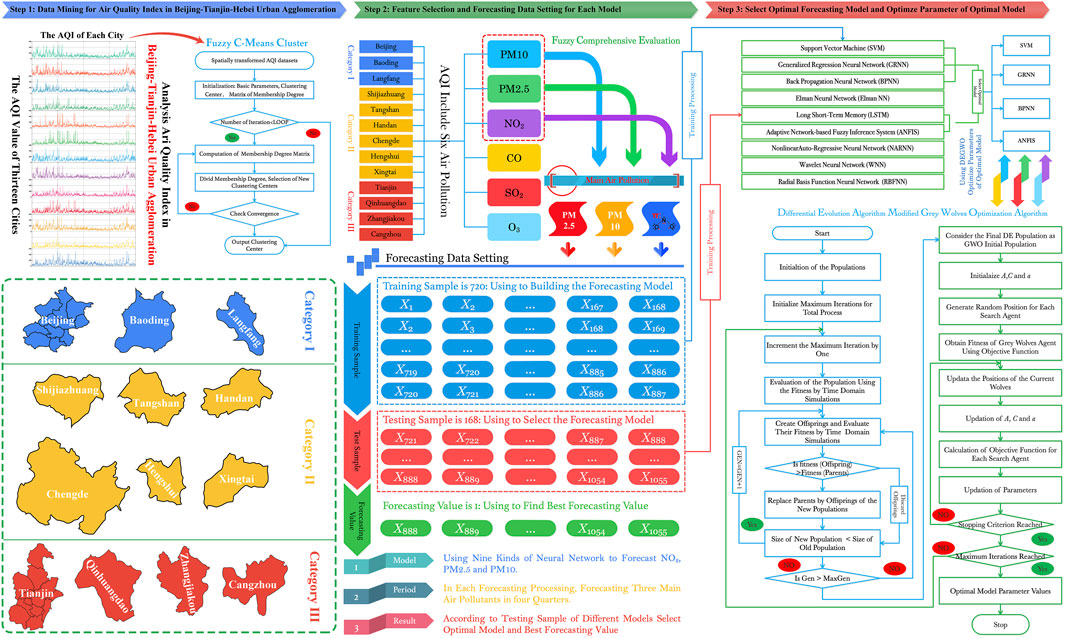
FIGURE 1. Flowchart of air quality index forecasting system for Beijing–Tianjin–Hebei Urban Agglomeration.

From the above, we can see that the AQI forecasting step using the hybrid forecasting system proceeds as follows:

Step 1: Data Mining

1. Collect the original data in the proposed hybrid forecasting model. Specifically, the average hourly AQI and six air pollutants are utilized as experiment data in this work.

2. Using data mining technology, 13 cities in Beijing–Tianjin–Hebei Urban Agglomeration (BJ-TJ-HE) are clustered, the characteristics of each category are summarized, and each category is further analyzed.

The AQI and six air pollution time series with missing points is filling processed by shape-preserving piecewise cubic spline interpolation, which maintains the continuity of each time series.

Step 2: Feature selection and data setting for each model

1. Feature selection: According to the result of cluster, establish fuzzy comprehensive evaluation for six pollutants and find out the main air pollutants of each in the same category.

2. Data setting: Each main air pollutants time series can be divided into three parts: training sample and testing samples for the forecasting values. The training sample is used to construct and train the ANNs, which in this work consist of a BPNN, SVM, GRNN, LSTM, and ANFIS. In addition, the testing sample is used to select the optimal model. For this, the WIC values of the ANNs are calculated, and the best model in terms of the WIC is selected. The input data are used to train the ANNs before calculating the forecasting value, with 1–6 input nodes and 1–30 hidden nodes. According to the value of WIC, the best forecasting model and best structure are chosen.

Step 3: Optimize the parameters of the best forecasting model.

To ensure the forecasting performance, a modified optimization algorithm is used to further optimize the parameters of the best forecasting model (expect LSTM). Finally, the main air pollutants forecasting results are obtained and compared with those of different hybrid forecasting models.

Experiment Design and Analysis

In this section, the specific information of experiment datasets in BJ-TJ-HE are described in detail. Eight performance metrics are applied to assess the performance of the proposed model. The experiments conducted in this study were implemented on Matlab 2018a, and the specifications of the hardware were as follows: Intel Core i9-7920X 2.90 GHz CPU and 32 GB RAM.

Data Description

The BJ-TJ-HE is the national capital region of the People's Republic of China. It is the biggest urbanized megalopolis region in Northern China, where Beijing, Tianjin, Baoding, and Langfang are the central core areas of BJ-TJ-HE. In this paper, the 13 cities of BJ-TJ-HE are evaluated to develop an early warning indicator for air quality. The datasets of hourly concentrations of the six major air pollutants used in this study are retrieved from the website of the China National Environment Monitoring Centre (http://www.cnemc.cn/sssj/). The first dataset includes AQI hourly concentrations collected from January 1, 2017, to December 31, 2018, in BJ-TJ-HE. Figure 2 shows the result of fuzzy C-mean cluster, which displays the construction of a fuzzy matrix based on the attributes of AQI in 13 cities and objectively and accurately cluster (Category I: Beijing, Baoding, Langfang; Category II: Shijiazhuang, Tangshan, Handan, Chengde, Hengshui, Xingtai; Category III: Tianjin, Qinhuangdao, Zhangjiakou, Cangzhou). The result of fuzzy comprehensive evaluation is shown in Table 1, which found that the main air pollutants are PM₁₀, PM₂, and NO₂ in 13 cities.

FIGURE 2

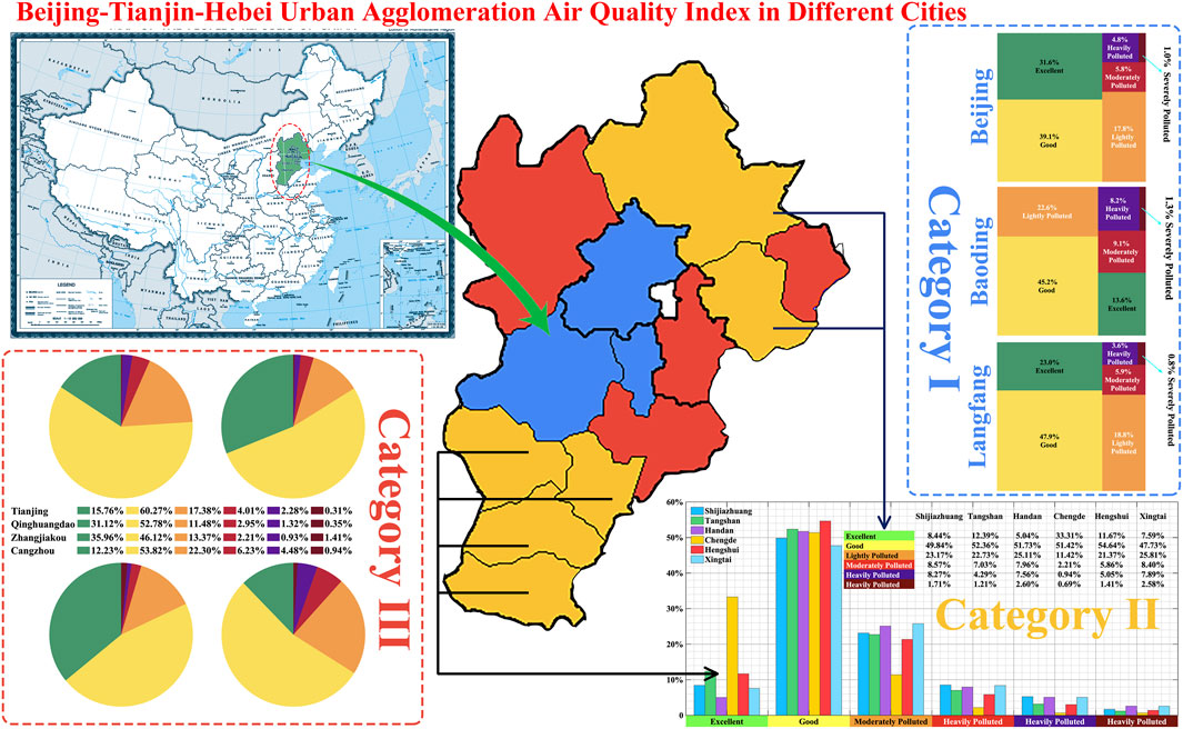
FIGURE 2. Result of data mining for Beijing–Tianjin–Hebei Urban Agglomeration.

TABLE 1

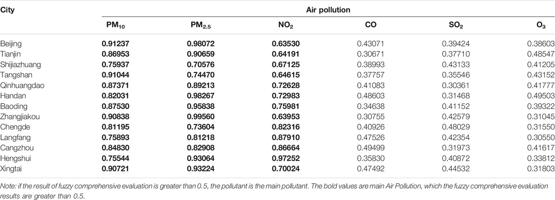
TABLE 1. The result of fuzzy comprehensive evaluation

According to the analysis in Table 1, the main air pollutants from statistical analysis of BJ-TJ-HE are NO₂, PM_2.5, and PM₁₀ shown in Table 2, in which the average value of the main air pollutants shows obvious differences among the 13 cities. The average value of NO₂ in the different cities is between 22.2525 and 49.4348 μg/m³, in which the average value in Xingtai is higher than in the other cities. At the same time, the PM_2.5 and PM₁₀ average values in Xingtai are 69.6938 and 135.8368 μg/m³, which are also higher than in the other cities. The maximum values of NO₂, PM_2.5, and PM₁₀ were in Hengshui, Baoding, and Zhangjiakou, with values of 215, 402, and 1581 μg/m³, and the minimum values of the three main air pollutants were in Zhangjiakou, Beijing, and Zhangjiakou, with values of 1, 3, and 12 μg/m³.

TABLE 2

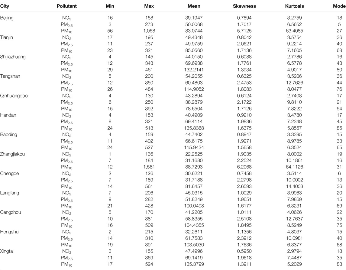
TABLE 2. Statistic of each main air pollutant in different cities.

In terms of skewness, all data sets are rightward, with values of skewness are greater than 0. For the values of kurtosis, only three data sets of NO₂ were less than 3, which meant that these three sets (Qinhuangdao, Shijiazhuang, and Xingtai) had a fat tail. At the same time, the other data sets had a thin tail.

Forecasting Metric

This section focuses on the efficiency of the different forecasting model with respect to computational performance. Eight evaluation criteria are applied to estimate the forecasting performance, namely, mean absolute error (MAE), root mean square error (RMSE), mean absolute percentage error (MAPE), Theil U statistic 1 (U1), and Theil U statistic 2 (U2) were calculated for all the fits; the goodness of forecasting fit (R²) and the standard of forecasting error (STDE) indicates the stability of the forecasting models; and the direction accuracy (DA) evaluates the optimal decision-making, often relying on correct forecasting directions or turning points between the actual and forecasting values. These performance metrics are defined in Table 3.

TABLE 3

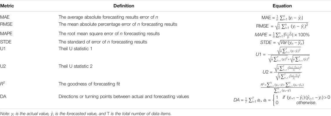
TABLE 3. Definition of the performance metrics.

Experiment Preparation: Model Selection

In the forecasting processing, there is no model that can be applied to all time series in the process of forecasting. Therefore, in this paper we developed a new metric, which measures accuracy of each hybrid model testing set and determines whether the model can provide the optimal forecasting value. The process of model selection is as follows:

Each model data is divided into 840 training samples, 168 testing samples, and one forecasting value. The accuracy of the testing sample is calculated by using the WIC. In order to eliminate the difference of the order of magnitude of forecasting metric, the MAE, MAE RMSE, MAPE, STDE, U1, and U2 are normalized. The calculation formula is as follows:

$\mathrm{WIC=NMAE+NRMSE+NMAPE+NSTDE+U1+U2+R2+}\left(\mathrm{1-DA}\right)$

For the first forecasting, the 1st to 840th samples are the training samples, the 841st to 1008th samples are the testing samples, and the 1009th sample is the forecasting value. At the end of the forecasting, the WIC value of the testing sample is calculated. If the WIC of the ith model is the smallest, the forecasting value of the ith model provides the optimal forecasting value.

For the second forecasting, the 2nd to 841st samples are the training samples, the 842nd to 1009th samples are the testing samples, and the 1010th sample is the forecasting value. At the end of the forecasting, the WIC value of the testing sample is calculated. If the WIC of the ith model is the smallest, the forecasting value of the ith model provides the optimal forecasting value.

For the kth forecasting, the kth to (840 + k − 1)th samples are the training samples, the (840 + k)th to (1008 + k − 1)th samples are the testing samples, and the (1008 + k)th sample is the forecasting value. At the end of the forecasting, the WIC value of the testing sample is calculated. If the WIC of the ith model is the smallest, the forecasting value of the ith model provides the optimal forecasting value.

In the whole forecasting process, 168 optimal forecasting values are generated, and 168*5 WIC values are generated at the same time. Table 4 only shows the optimal model and the percentage of optimal forecasting value for three main air pollutants.

TABLE 4

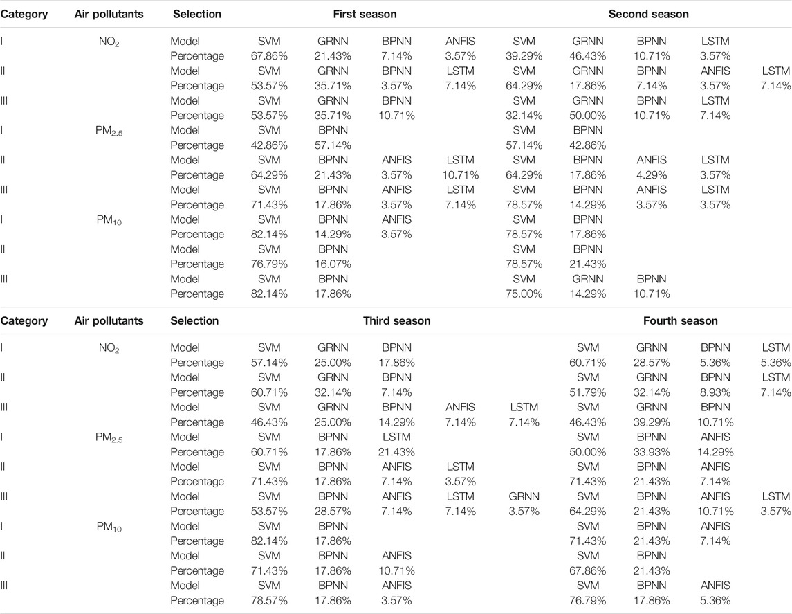
TABLE 4. The result of model selection for main air pollutants in different seasons.

From Table 4, it can be seen that SVM provides more optimal forecasting value for the three main pollutants at different times, especially in the PM₁₀ forecasting process; the optimal forecasting value for the first quarter and the third quarter is 82.14% (138 optimal forecasting value), and the other four models also provide corresponding optimal forecasting value.

Experiment I: Forecasting Processing for Three Categories of NO₂ by Each Model in the First Season

In this portion, the hourly NO₂ time series for 13 cities in three categories were utilized as the testing data for the five hybrid models with one-step-ahead forecasting. Beyond that, with the purpose of comprehensively comparing the precision of the modeling forecasting, this experiment consisted of two parts: the multi-step forecasts demonstrated in Table 4 and, for the local analysis horizon, the local forecasts presented in Table ′5 and Figure 3, which focus on first season. Table 5 and Figure 3 demonstrate the following:

1) Focusing on Category I, the new proposed model based on model selection realizes excellent results on the eight evaluation indices in the first season forecasting. On the contrary, DEGWO-ANFIS has the lowest effectiveness. The maximum reduction of MAPE for the proposed model compared with the other hybrid models is approximately 71.18% in Beijing's NO₂ forecasting, 53.93% in Baoding's NO₂ forecasting, and 61.61% in Langfang's NO₂ forecasting, respectively. The reduction was about 62.39% and 76.49% for one-step forecasting and 2.79%, 6.10%, and 19.33% for the three cities at the hourly interval NO₂ forecasting in Category I. As for the R², the proposed model has the best performance among the four single-hybrid models for hourly interval NO₂ time series.

2) Focusing on Category II, it is clear that proposed model based on model selection exhibits the best performance among the single fourth hybrid models implemented for all eight criteria involved. For the MAPE, there are average reductions between the proposed model and single hybrid model, by approximately 12.48%, 29.12%, 60.00%, and 66.70% in six cities for the hourly NO₂ time series forecasting, respectively. Comparing the four single hybrid models for the hourly NO₂ forecasting, the forecasting accuracy of DEGWO-SVM is higher than that of the other three hybrid models. The average reduction of MAPE among the MODEGWO-SVM and the other three hybrid models is 16.70%, 42.79%, and 50.10%, respectively. In addition, all the R² values of the proposed model are over 90%, which underlines the higher fitting effect on Category II.

3) The forecasting metric of the single hybrid models and the proposed model in Table 4 indicates that the proposed model based on model selection performs better than the single hybrid model in Category III. As an example, with respect to Tianjin, the DA values of the individual hybrid models are 80.84% (MODEGWO-SVM), 70.06% (MODEGWO-GRNN), and 77.84% (MODEGWO-BPNN), while the DA values of the proposed models is 87.24%, respectively. The comparative analysis between the proposed model and the single model confirms the advantages of the hybrid forecasting model.

4) Moreover, Table 5 displays each metric of NO₂ forecasting among the developed hybrid forecasting system and the single hybrid models. According to Table 5, it is obvious that the values of MAE, RMSE, MAPE, U1, and U2 of the proposed hybrid model are all smaller than the other considered models, and the values of DA and R² of the developed hybrid forecasting system are all greater than that of the single hybrid model, which further confirms the superiority of the presented hybrid forecasting system in terms of forecasting ability.

TABLE 5

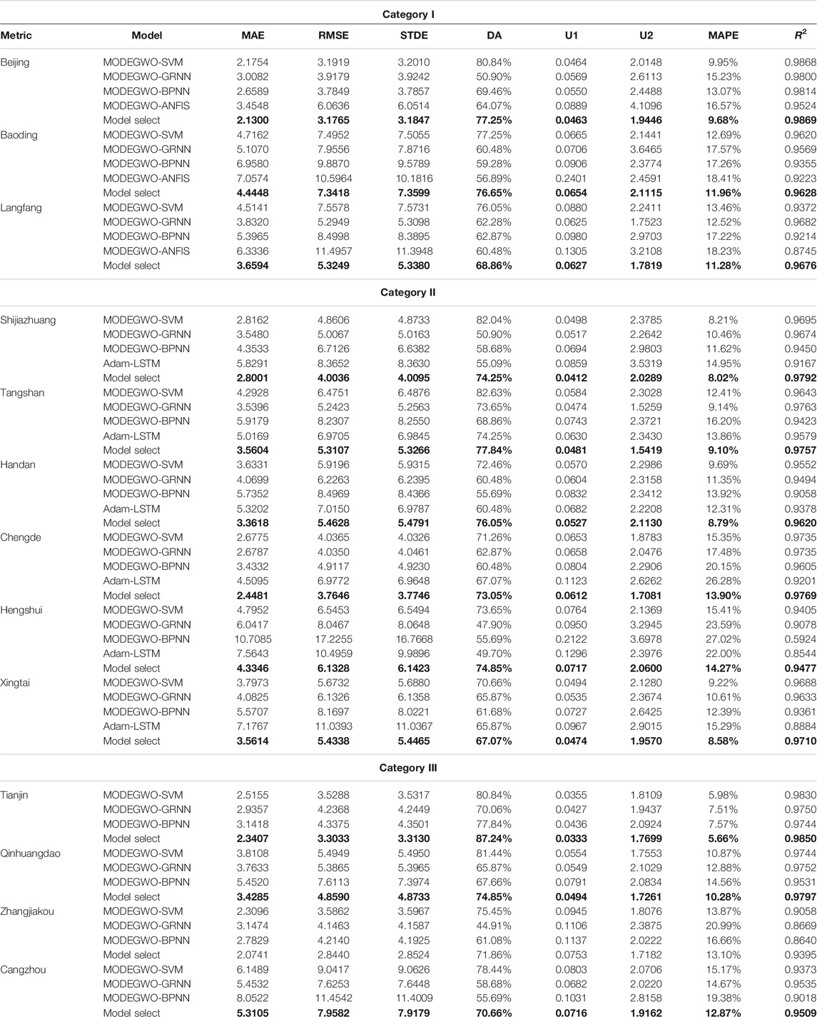
TABLE 5. The forecasting results of each model for NO₂ in three categories.

FIGURE 3

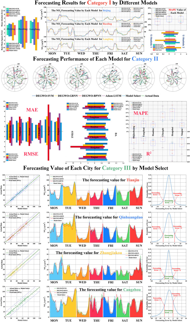
FIGURE 3. Forecasting result of NO₂ for three categories in the first season.

In summary, from the analyses above, it can be concluded that the model selection forecasting system realizes the best forecasting results compared to the single hybrid model. Model selection also gives better forecasting performance in the other season with the results shown in Supplementary Appendices S2–S4 indicating better robustness of the model selection forecasting system.

Experiment II: The Forecasting Results of Category II PM_2.5 Forecasting in the First Season

This experiment mainly focused on the forecasting performance of each model for PM_2.5 of Category II in the first season, with the forecasting results of four different hybrid models (MODEGWO-SVM, MODEGWO-BPNN, MODEGWO-ANFIS, Adam-LSTM) and model selection represented in Table 6 and Figure 4

1) For first season PM_2.5 forecasting accuracy, the final forecast results of PM_2.5 for six cities in Category II are composed of four hybrid models, which include MODEGWO-SVM, MODEGWO-BPNN, MODEGWO-ANFIS, and Adam-LSTM. Among the four models, MODEGWO-SVM and MODEGWO-BPNN have better forecasting performance, with the MODEGWO-SVM obtaining 64.29% optimal forecasting points and the MODEGWO-BPNN obtaining 21.43% optimal points for six cities in Category II. The smallest MAPE values of MODEGWO-SVM are 0.92%, 0.94%, 1.36%, and 0.79% for Hengshui, Tangshan, Chengde, and Xingtai PM_2.5 forecasting, and the MODEGWO-BPNN obtains the best MAPE (1.08% and 0.85%) value for Shijiazhuang and Handan.

2) For the goodness of fit, the R² values of four different hybrid models are over 0.95 for six cities in the first season, which indicates that the forecasting values obtained by these models is close to the actual value. The forecasting result of Shijiazhuang shows that the R² value of best hybrid modes (MODEGWO-BPNN) is 0.9993, very close to 1, which indicates that there is less difference between forecasting data and actual data, and the forecasting value is basically consistent with the actual value. Meanwhile, The DA values of the best hybrid model are over 70%, which proves the best models can effectively capture the changing trend of the actual data.

3) For the forecasting results of model selection, Table 6 and Figure 4 clearly show that the forecasting performance of model selection is better than the hybrid model. The MAPE value of model selection is 0.88%; compared with the optimal hybrid model the MAPE improved 22.73%, and the MAE and RMSE reduced 26.49% and 30.69%, respectively. Although the model selection can improve the forecasting accuracy, in the PM_2.5 forecasting of some cities, due to the better forecasting performance of the single hybrid model, the forecasting accuracy of the model selection is not significantly improved. For example, in the PM_2.5 forecasting of Xingtai, the MAPE value of optimal forecasting model (MODEGWO-SVM) is 0.79%, and the MAPE of the model selection is 0.76%, which shows that forecasting accuracy has no significant improvement.

4) Similar to the first season, the PM_2.5 forecasting results of Category II in the second to fourth seasons are listed in Supplementary Appendix Table 7 in which the best forecasting performances of the hybrid model are shown by DEGWO-SVM, DEGWO-BPNN, DEGWO-ANFIS, and Adam-LSTM for PM_2.5 forecasting in each city. Compared with the optimal hybrid model, the final forecasting results obtained by the model selection is more accurate than single hybrid model, which indicates that the optimal hybrid model has good forecasting performance but cannot be applied to all the forecasting data.

TABLE 6

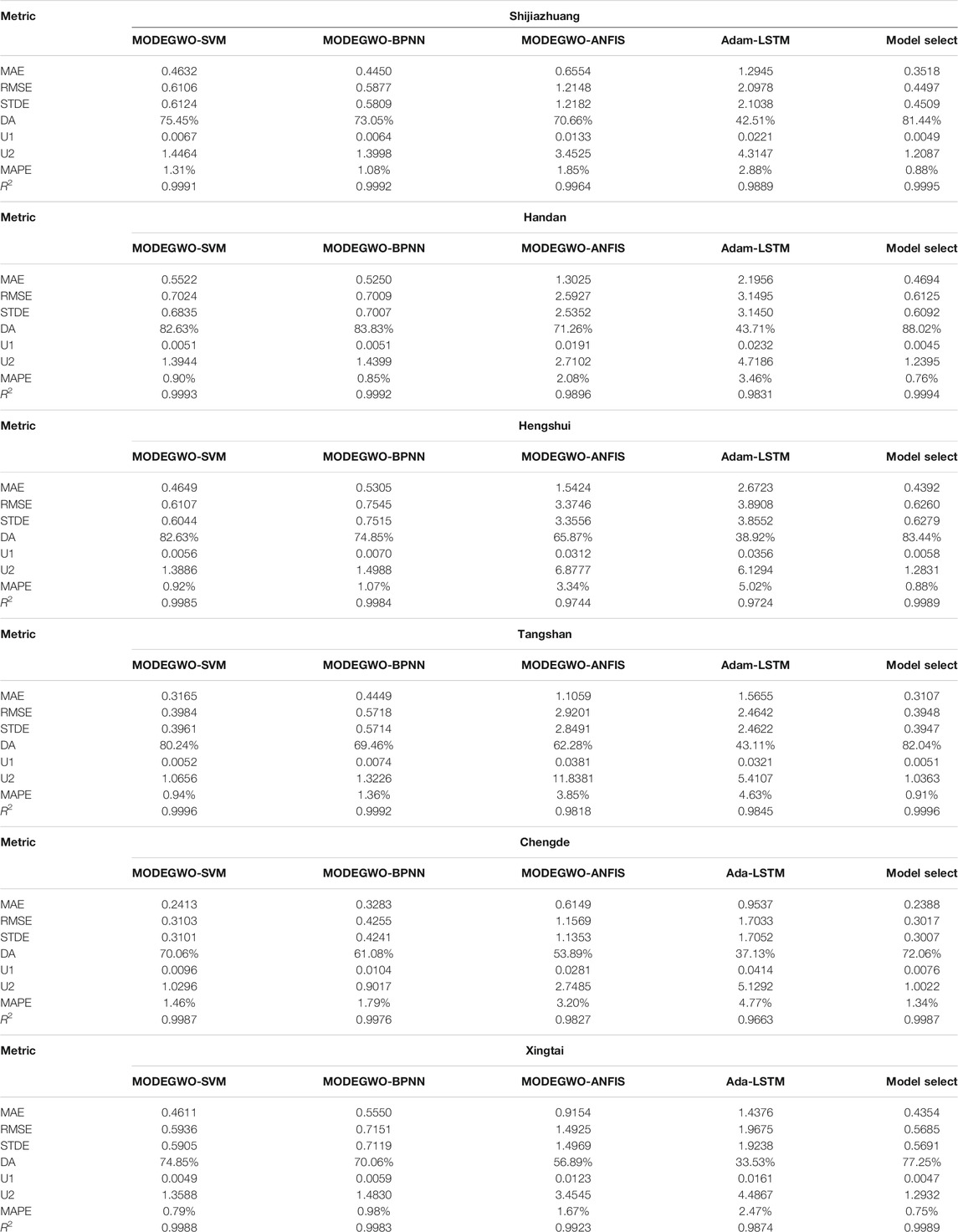
TABLE 6. The PM_2.5 forecasting result for each city in Category II by different models.

FIGURE 4

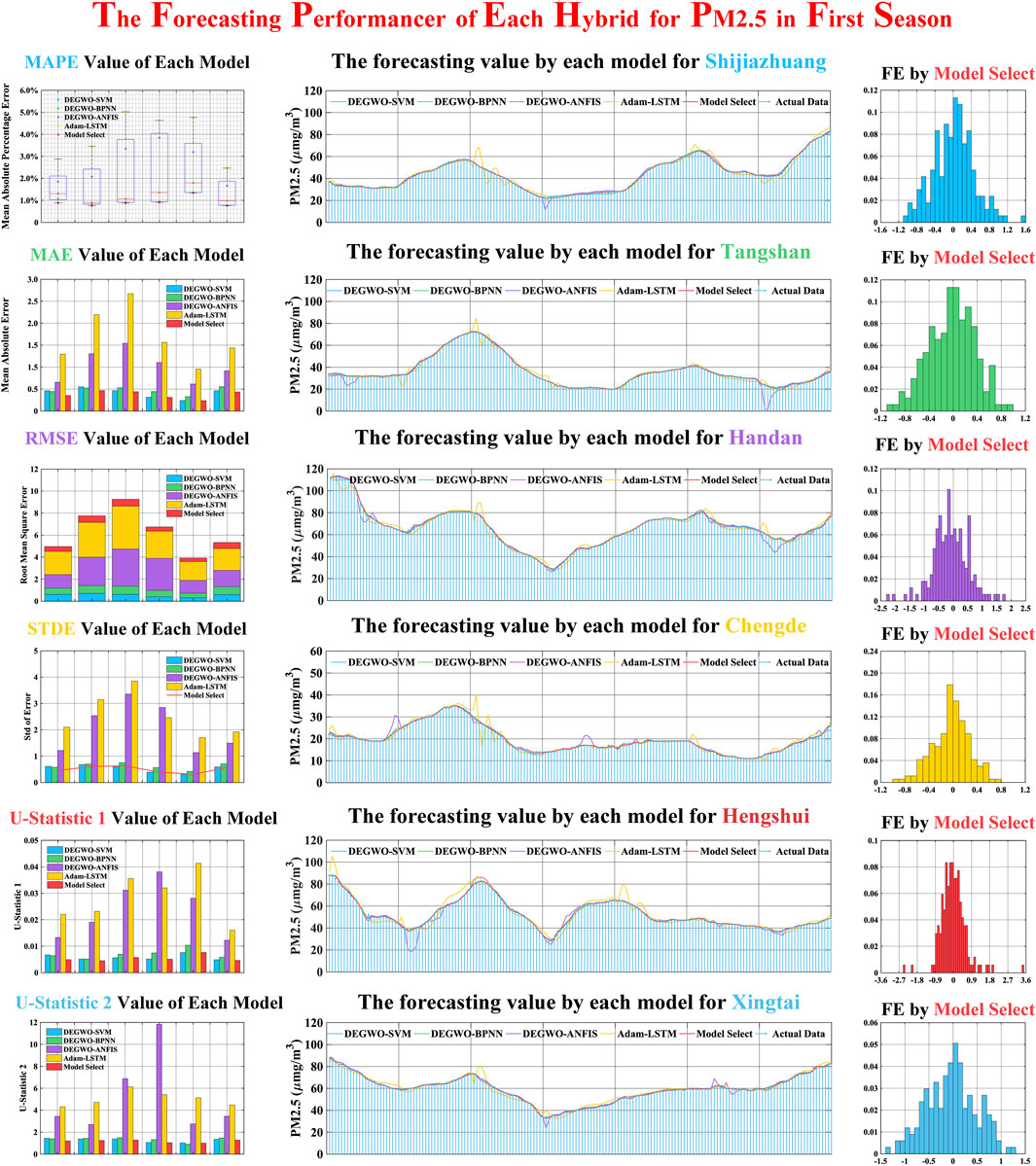
FIGURE 4. Forecasting performance of each model for Category II in the first season.

In summary, for the Category I and Category III PM_2.5 forecasting list in Supplementary Appendices S5–S7, the model selection forecasting system exhibits the best forecasting accuracy among the different hybrid models for four seasons. It is evident that the forecasting capacity of the model selection is robust when considering each forecasting metrics. The accuracy of model selection depends on the hybrid model, so it is necessary to increase the types of models in the modeling process which ensures that more forecasting results can be obtained, and the optimal forecasting value can be selected in the model selection process.

Experiment III: PM₁₀ Forecasting Analysis for Category III in Four Seasons

For the hourly PM₁₀ time series for three categories, it can be observed that the model selection forecasting system attains satisfactory results. Specifically, the lowest values of MAE are 0.4643, 0.4600, and 0.3869 and of RMSE are 0.7302, 0.7906, and 0.5561, corresponding to PM₁₀ forecasting in Category I in three cities, successively. The results of Category I indicate that the smaller the MAE and MSE, the smaller the deviation between the observations and forecasting, which verifies the forecasting performance. In addition, the average MAPE values of model selection for six cities of Category II in four seasons are lower than 1%. Compared with the optimal hybrid model, the model selection is approximately reduced by 10%. The analyses reveal the forecasting superiority of the model selection system. By parity of reasoning, a similar conclusion can be reached through the analyses of the hourly PM₁₀ forecasting results for Category III (the forecasting results are shown in Table 7 and Figure 5).

1) For PM₁₀ forecasting in the first season, the optimal hybrid models are DEGWO-SVM and DEGWO-BPNN, with which the MAPE values of the best hybrid model (DEGWO-SVM) for four cities of Category III are 0.71%, 0.81%, 1.09%, and 0.72%. The final forecasting values are obtained by model selection; based on the results of DEGWO-SVM and DEGWO-BPNN the MAPE values of model selection are 0.65%, 0.75%, 0.97%, and 0.67%. Additionally, the values of other forecasting metrics are at their best under the model selection.

2) In the second season of PM₁₀ forecasting for four cities, the final forecasting results consist of four different hybrid models (DEGWO-SVM, DEGWO-GRNN, DEGWO-BPNN, and DEGWO-ANFIS). From the forecasting performance of four hybrid models, the forecasting performance of DEGWO-SVM is better than the other three models, in which the values of MAPE are 2.65%, 0.86%, 2.27%, and 2.83% for different cities' PM₁₀ forecasting in Category III. Additionally, the DA value of MODEGWO-SVM is over 75%, which indicates that the hybrid model can capture future changing trends of PM₁₀. The final forecasting results are obtained by model selection, in which the forecasting accuracy is better than those of the four hybrid models. Compared with the best hybrid model, the MAPE values of model selection are reduced by 25.00%, 2.38%, 10.19%, and 69.46%, respectively.

3) According to forecasting results in Table 7 and Figure 5 for PM₁₀ of the third season, the three kinds of hybrid models (DEGWO-SVM, DEGWO-BPNN, and DEGWO-ANFIS) are employed to forecast hourly PM₁₀; the DEGWO-SVM has the best forecasting performance among the three hybrid models in Zhangjiakou, and the MAPE is 0.61%. DEGWO-SVM has better forecasting accuracy, and model selection has little improvement on the forecasting accuracy in the final prediction results, but the MAPE has maximum improvement of 29.76% for Tianjin PM₁₀ forecasting.

4) According to the results in Table 6, the three kinds of hybrid models are used to forecast PM₁₀ for four cities of Category III in the fourth season, and the R² value of each model was greater than 0.99, which shows that these models have a good forecasting performance for the PM₁₀. Meanwhile, model selection uses the predicted values of each model to form the final forecasting results, and the corresponding MAE values are 0.5747, 0.6459, 0.7297, and 0.6300 for four cities.

TABLE 7

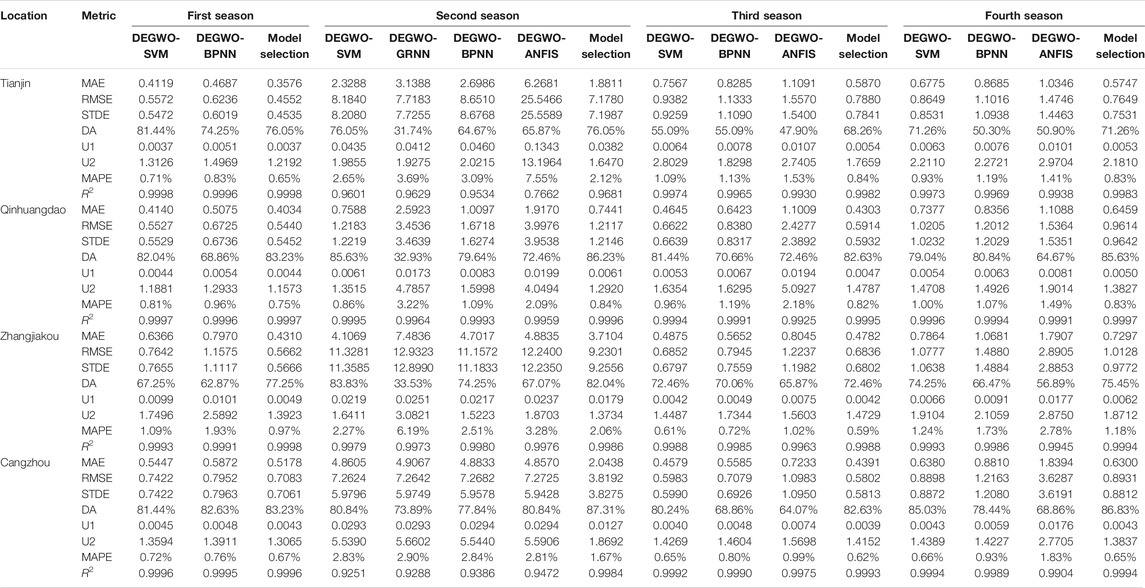
TABLE 7. The forecasting result of each model in different seasons for Category III.

FIGURE 5

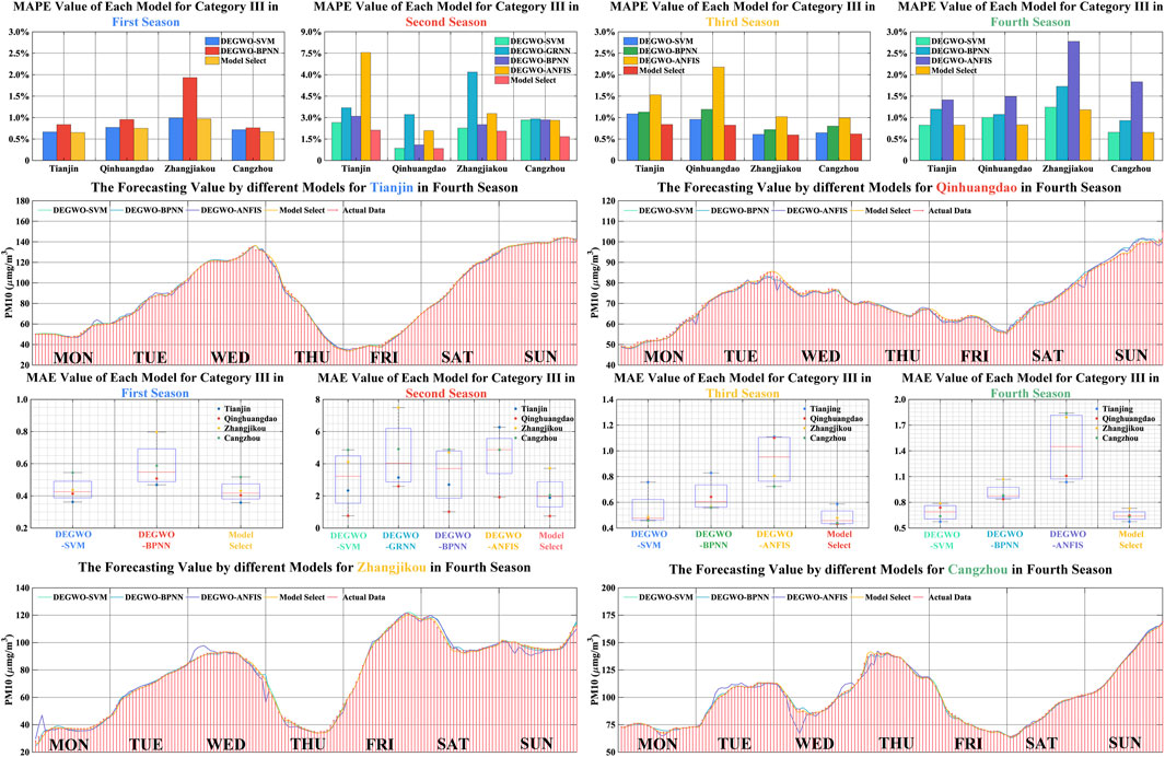
FIGURE 5. The forecasting result of PM₁₀ for Category III in different seasons.

In summary, whether for Category III or the other categories (the results are shown in Supplementary Appendix S8 and Supplementary Appendix S9) PM₁₀ forecasting, the model selection system attained the best performance for 13 cities. In the comparison of various hybrid models, the forecasting performance of MODEGWO-SVM is better than other hybrid models. Additionally, it can be observed that some models have low accuracy, which can still provide some optimal forecasting values for the model selection system for hourly PM₁₀ forecasting. Based on the above analysis, it can be seen that none of the models has been playing the best forecasting performance in the forecasting process, and various hybrid models are needed to make up for the shortcomings of the single hybrid model.

Discussions

This section mainly discusses the hyperparameter related to the SVM and ANN model that would influence the forecasting performance. A large variety of machine learning models and ANNs are available for air pollution time series including three different type pollutants. Finally, compare computing in different model.

Support Vector Machine

According to the results of each experiment, SVM provided the more optimal forecast values for the three main pollutants in the four quarters of 13 cities. The reason for the favorable score produced by SVM is that SVM provides a way to avoid the complexity of high-dimensional space by directly using the inner product function of the space (which is the kernel function) and then directly solving the corresponding decision-making problem in high-dimensional space by using the solution method under the condition of linear separability. When the kernel function is known, it can simplify the difficulty of solving the problem in high-dimensional space. Meanwhile, SVM is based on the small sample statistical theory, which conforms to machine learning. In addition, support vector machine has better generalization ability than neural network. Although the time series of the three main air pollutants are neither regular nor seasonal, SVM can also effectively capture future changes of the three main air pollutants.

SVM has two very important parameters: c and g. c is the penalty coefficient, that is, tolerance of errors. The higher the c, the more intolerable the errors and easy to over-fit. The smaller the c, the less easy fitting is. If c is too large or too small, the generalization ability becomes worse. g is a parameter that comes with RBF function when it is selected as a kernel. Implicitly it determines the distribution of data after mapping to a new feature space. The bigger the g, the less support vectors; it will only act near the support vector samples. For the unknown samples, the classification effect is very poor. There is a possibility that the training accuracy can be very high, and the test accuracy is not high, that is, over-fitting. The smaller the g value is, the more support vectors there are, and the greater the smoothing effect will be; the higher accuracy of the training processing cannot be obtained, and the accuracy of the testing processing will also be affected. This paper used DEGWO algorithm and GWO algorithm to optimize the parameters of SVM (c and g). The results of two types of hybrid SVMs are shown in Table 8, which displays that the optimum penalty coefficients of SVM corresponding to pollutant forecasting in different cities vary widely. For example, in the forecasting processing of NO₂, the variation range of parameters is [2, 99]. However, the fluctuation range of g is small, with most variations ranging from 0 to 1. In general, the air pollutants forecasting performances of support vector machine are very dependent on the penalty coefficient. In the whole experiment it can be observed that the support vector machine has good forecasting accuracy for three main air pollutants forecasting, but it cannot provide the best forecasting value in each point. It indicates that the support vector machine is suitable for hourly air pollutants forecasting.

TABLE 8

TABLE 8. The result of two types of SVM for three main air pollutants in different cities.

Artificial Neural Network: Number of Input Layer and Number of Hidden Layers

ANN as a nonlinear mapping model is used to solve the problem of time series forecasting, because the ANN model can find the optimal solution of a complex problem with the help of high-speed computing ability of the computer. In order to ensure the forecasting accuracy of the ANN model, parameters of ANN need to be elaborately configured. However, there is no effective rule for establishing the values of these parameters on air pollutants forecasting. Although there are many studies on the tuning of the parameters of the neural network, it is obvious that the selection of the whole parameter space is beyond the scope of this study. Therefore, the parameters of the neural network are set by means of simulation experiment and optimization algorithm: the experimental design is as follows:

This processing configured various input layers and a number of hidden layers to find out the influence of the usage of recent data on the performance of different ANN models. The number of input layers from 1 to 10 increases for three main air pollutants, which means there are 1,008 pieces of sample data on NO₂, PM_2.5, and PM₁₀; the train-to-verify ratio 5:1 means that 840 pieces of sample data were used as training data for building the ANN model, while 168 pieces of sample data were used as testing data for finding the training-to-testing ratio and parameter of each ANN model (the optimal number of input layers of each model and the number of hidden layers of LSTM and BPNN). Figure 6 shows the forecasting performance with the different configurations of the optimal number of input layers and the number of hidden layers of LSTM and BPNN, in which it is difficult to find a regular correlation between the forecasting performances and the parameters. Consequently, it is difficult to find an optimal combination of ANN's parameters that brings the model to the best performance in the practical air pollutant forecasting where MAPE and R² are unknown.

FIGURE 6

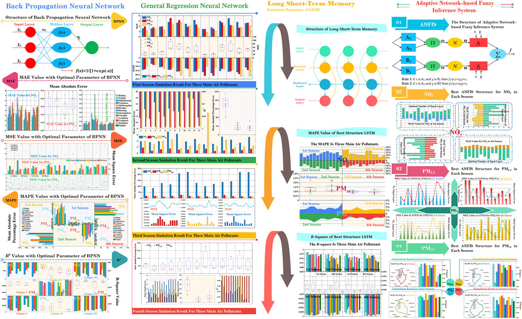
FIGURE 6. The simulation result of each ANN model for three main air pollutants in different cities.

During the experiment on configurations of ANN's parameter, the optimal parameter setting trained the networks models for each ANN model in 13 cities. The forecasting values with the best performance of each ANN (the best forecasting metric in Table 9) were selected to forecast three main air pollutants in each experiment. However, it can be found that there were no giant differences on forecasting performance among the networks trained with the same configuration, even if the neural network has the randomness and probability mechanism inside the training processing. A large sample of the times series is another reason that the training stability of the neural network can be ensured. For example, the best MAPE of BPNN for the forecasting of NO₂ in Beijing shown in Figure 6 is 5.82%, and the worst one is 8.94%. Most of the MAPEs are between 6% and 7%. It is practical to use ANN in real air pollutants forecasting application where forecasting the changing air pollutant time series is suitable.

TABLE 9

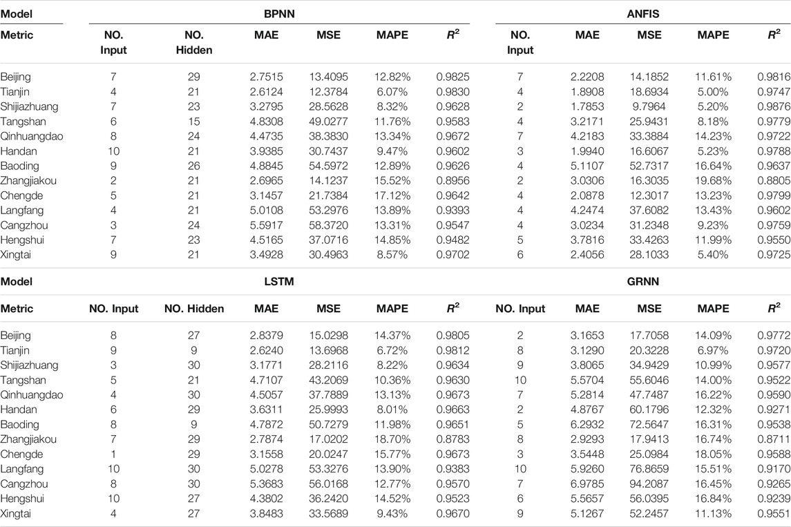
TABLE 9. The simulation result of each ANN model.

In summary, with the rapid development of ANN, it has become a powerful tool to solve prediction problems. Neural network is used in the field of air pollution to solve the problem of non-linear forecasting which cannot be solved by statistical models. Its non-linear mapping is especially suitable for the application of air pollutant forecasting. The main reason is that the ANN has the following advantages:

1) Non-linear mapping ability: ANN realizes a mapping function from input to output in essence. Mathematical theory proves that three-layer neural network can approximate any non-linear continuous function with arbitrary precision. This makes it especially suitable for solving complex internal mechanism problems, that is, ANN has strong non-linear mapping ability.

2) Self-learning and self-adapting ability: ANN can automatically extract the “reasonable rules” between output and output data by learning and self-adaptively memorizing the learning content in the weights of the network. ANN has a high ability of self-learning and self-adaptation.

3) Generalization ability: When designing pattern classifiers, the so-called generalization ability refers to whether the network can forecast the unknown time series correctly after training, while ensuring that the classified objects are correctly classified. ANN can apply learning results to new knowledge.

4) Fault-tolerant ability: ANN will not have a great impact on the global training results after its local or partial neurons are damaged; the system can work normally even when it is damaged locally. ANN has certain fault-tolerant ability.

Computing Time for Each Model

In order to improve the computing efficiency and save the computing time, training and forecasting processing of all the models for the main air pollutants time series with parallel computing by central processing unit (CPU) and graphics processing unit (GPU). The computing times of every independent hybrid model in each experiment are shown in Table 10, from which we can further research the computational efficiency of the developed model selection forecasting system for the main air pollutants. Specifically, the average computation time of the model selection forecasting system ranges from 330.6037 to 363.2167 s for NO₂ forecasting in Category II, with the longest computing time appearing in the different categories. Notably, Adam-LSTM with complex model structure has longer computing time than the other hybrid models, taking more time in the iterative optimization process. Moreover, this paper establishes multiple hybrid models and uses the model selection method to find the best forecasting value, in which the final forecasting accuracy is improved but needs more computing time.

TABLE 10

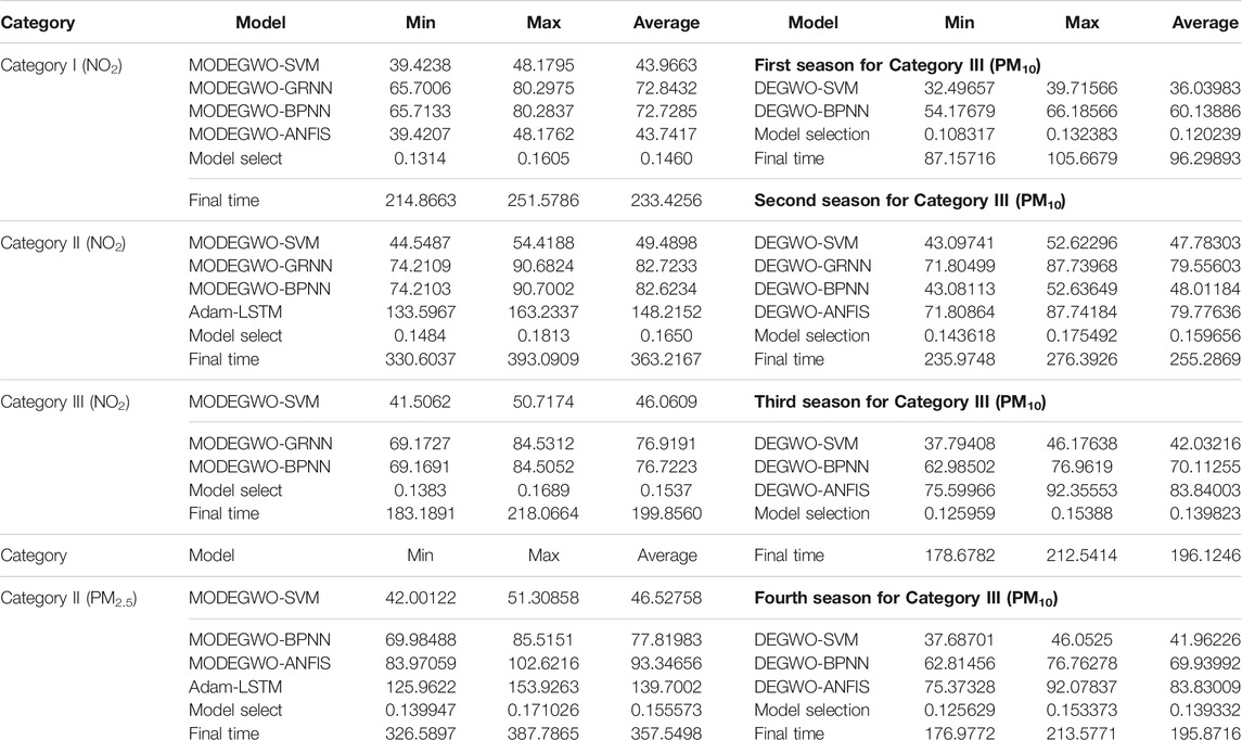
TABLE 10. Computing time by each model.

Conclusion

In this study, a novel model selection forecast system was proposed that overcomes the shortcomings of the single hybrid model, which cannot give the optimal results for the forecasting process. First, the FSE theory is employed to analyze the major pollutant for each city in BJ-TJ-HE, and the fuzzy c-means algorithm is used to analyze the feature of the 13 cities. Then, to further improve modeling accuracy and rationality of modeling, a modified optimization algorithm (DEGWO) was used to optimize the premasters of different models. Finally, the model selection forecasting system obtains forecasting results at each time point from different hybrid models.

The developed model selection forecasting system was evaluated on hourly NO₂, PM_2.5, and PM₁₀ from 13 cities, and several performance metrics were calculated, with experimental results indicating that the model selection forecasting system is superior to single hybrid models with the smallest MAPE in the different cities pollutant forecasting, indicating its strong forecasting performance. Overall, the proposed model selection forecast system exhibits outstanding performance in data analysis and time series forecasting for air pollutants. Specifically, it can not only deeply analyze major pollutants of AQI for BJ-TJ-HE but also approximate the actual values with high accuracy and stability.

Data Availability Statement

The original contributions presented in the study are included in the article/Supplementary Material, further inquiries can be directed to the corresponding authors.

Author Contributions

The design experiment, data analysis, and paper writing were conducted by YH; the forecasting experiment and data analysis were completed by YH and CW; supervision, paper writing, and editing were conducted by CW and YD; validation, methodology, paper editing, and supervision were handled by QL and GZ. All authors have read and agreed to the published version of the manuscript.

Funding

This work was supported by Western Project of the National Social Science Foundation of China (Grant No. 18XTJ003).

Conflict of Interest

The authors declare that the research was conducted in the absence of any commercial or financial relationships that could be construed as a potential conflict of interest.

Publisher’s Note

All claims expressed in this article are solely those of the authors and do not necessarily represent those of their affiliated organizations, or those of the publisher, the editors and the reviewers. Any product that may be evaluated in this article, or claim that may be made by its manufacturer, is not guaranteed or endorsed by the publisher.

Supplementary Material

The Supplementary Material for this article can be found online at: https://www.frontiersin.org/articles/10.3389/fenvs.2021.761287/full#supplementary-material

References

Akyüz, M., and Çabuk, H. (2009). Meteorological Variations of PM2.5/PM10 Concentrations and Particle-Associated Polycyclic Aromatic Hydrocarbons in the Atmospheric Environment of Zonguldak, Turkey. J. Hazard. Mater. 170, 13–21. doi:10.1016/j.jhazmat.2009.05.029

CrossRef Full Text | Google Scholar

Bessagnet, B., Couvidat, F., and Lemaire, V. (2019). A Statistical Physics Approach to Perform Fast Highly-Resolved Air Quality Simulations – A New Step towards the Meta-Modelling of Chemistry Transport Models. Environ. Model. Softw. 116, 100–109. doi:10.1016/j.envsoft.2019.02.017

CrossRef Full Text | Google Scholar

Brereton, R. G., and Lloyd, G. R. (2010). Support Vector Machines for Classification and Regression. Analyst 135, 230–267. doi:10.1039/b918972f

PubMed Abstract | CrossRef Full Text | Google Scholar

D'Allura, A., Kulkarni, S., Carmichael, G., Finardi, S., Adhikary, , , Wei, , et al. (2011). Meteorological and Air Quality Forecasting Using the WRF–STEM Model during the 2008 ARCTAS Field Campaign. Atmos. Environ. 45. doi:10.1016/j.atmosenv.2011.02.073

CrossRef Full Text | Google Scholar

Dass, A., Srivastava, S., and Chaudhary, G. (2021). Air Pollution: A Review and Analysis Using Fuzzy Techniques in Indian Scenario. Environ. Technology Innovation 22, 101441. doi:10.1016/j.eti.2021.101441

CrossRef Full Text | Google Scholar

Davood, N.-K., Goudarzi, G., Taghizadeh, R., Asumadu-Sakyi, A., and Fehresti-Sani, M. (2021). Long-term Effects of Outdoor Air Pollution on Mortality and Morbidity–Prediction Using Nonlinear Autoregressive and Artificial Neural Networks Models. Atmos. Pollut. Res. 12, 46–56. doi:10.1016/j.apr.2020.10.007

CrossRef Full Text | Google Scholar

Dhiman, G., and Kumar, V. (2018). Multi-objective Spotted Hyena Optimizer: A Multi-Objective Optimization Algorithm for Engineering Problems. Knowledge-Based Syst. 150, 175–197. doi:10.1016/j.knosys.2018.03.011

CrossRef Full Text | Google Scholar

Díaz-Robles, L. A., Ortega, J. C., Fu, J. S., Reed, G. D., Chow, J. C., Watson, J. G., et al. (2008). A Hybrid ARIMA and Artificial Neural Networks Model to Forecast Particulate Matter in Urban Areas: The Case of Temuco, Chile. Atmos. Environ. 42, 8331–8340. doi:10.1016/j.atmosenv.2008.07.020

CrossRef Full Text | Google Scholar

Feng, X., Li, Q., Zhu, Y., Hou, J., Lingyan, J., and Wang, J. (2015). Artificial Neural Network Forecasting of PM2.5 Pollution Using Air Mass Trajectory Based Geographic Model and Wavelet Transformation. Atmos. Environ. 107, 118–128. doi:10.1016/j.atmosenv.2015.02.030

CrossRef Full Text | Google Scholar

Gayen, S., and Biswas, A., (2021). Pythagorean Fuzzy C-Means Clustering Algorithm. In Computational Intelligence in Communications and Business Analytics Cham. Editors J. K. Mandal, and S. Mukhopadhyay.

CrossRef Full Text | Google Scholar

Güçlü, Y. S., Dabanlı, İ., Şişman, E., and Şen, Z. (2019). Air Quality (AQ) Identification by Innovative Trend Diagram and AQ index Combinations in Istanbul Megacity. Atmos. Pollut. Res. 10, 88–96. doi:10.1016/j.apr.2018.06.011

CrossRef Full Text | Google Scholar

Han, Y., Lam, J. C., Li, V. O., and Reiner, D. (2021). A Bayesian LSTM Model to Evaluate the Effects of Air Pollution Control Regulations in Beijing, China. Environ. Sci. Pol. 115, 26–34. doi:10.1016/j.envsci.2020.10.004

CrossRef Full Text | Google Scholar

Hao, Y., Niu, X., and Wang, J. (2021). Impacts of Haze Pollution on China's Tourism Industry: A System of Economic Loss Analysis. J. Environ. Manag. 295, 113051. doi:10.1016/j.jenvman.2021.113051

CrossRef Full Text | Google Scholar

Hao, Y., and Tian, C. (2018). The Study and Application of a Novel Hybrid System for Air Quality Early-Warning. Appl. Soft Comput., 74.

Google Scholar

Hao, Y., Tian, C., and Wu, C. (2019). Modelling of Carbon price in Two Real Carbon Trading Markets. J. Clean. Prod. 244, 118556.

Google Scholar

Jang, J.-S. R. (1993). Anfis: Adaptive-Network-Based Fuzzy Inference System. IEEE Trans. Syst. Man. Cybern. 23, 665–685. doi:10.1109/21.256541

CrossRef Full Text | Google Scholar

Jiang, P., Dong, Q., and Li, P. (2017). A Novel Hybrid Strategy for PM 2.5 Concentration Analysis and Prediction. J. Environ. Manage. 196, 443–457. doi:10.1016/j.jenvman.2017.03.046

CrossRef Full Text | Google Scholar

Kim, J., Kim, D., Choi, M., and Choi, M. (2018). Impact of Air Pollution on Cause-specific Mortality in Korea: Results from Bayesian Model Averaging and Principle Component Regression Approaches. Sci. total Environ. 636, 1020–1031.

PubMed Abstract | Google Scholar

Kumar, K., Zindani, D., and Davim, J. P. (2019). Particle Swarm Optimization Algorithm. Optimizing Engineering Problems through Heuristic Techniques. 23–32. doi:10.1201/9781351049580-3

CrossRef Full Text | Google Scholar

Land, W. H., and Schaffer, J. D. (2020). The Generalized Regression Neural Network Oracle. The Art and Science of Machine Intelligence, 77–105. doi:10.1007/978-3-030-18496-4_3

CrossRef Full Text | Google Scholar

Lanzafame, R., Monforte, P., Patanè, G., and Strano, S. (2015). Trend Analysis of Air Quality Index in Catania from 2010 to 2014. Energ. Proced. 82, 708–715. doi:10.1016/j.egypro.2015.11.796

CrossRef Full Text | Google Scholar

Latif, M. T., Ahamad, F., Abdul Halim, N. D., Khan, M., Juneng, L., Chung, J. X., et al. (2018). The Long-Term Assessment of Air Quality on an Island in Malaysia. Heliyon 4, 1–33.

CrossRef Full Text | Google Scholar

Lauriks, T., Longo, R., Baetens, D., Derudi, M., Parente, A., Bellemans, A., et al. (2020). Application of Improved CFD Modeling for Prediction and Mitigation of Traffic-Related Air Pollution Hotspots in a Realistic Urban Street. Atmos. Environ. 246, 118127. doi:10.1016/j.atmosenv.2020.118127

CrossRef Full Text | Google Scholar

Leong, W. C., Kelani, R. O., and Ahmad, Z. (2019). Prediction of Air Pollution index (API) Using Support Vector Machine (SVM). J. Environ. Chem. Eng. 8, 103208.

Google Scholar

Li, W. k., Wang, W., Wang, Z., and Li, L. (2019). Opposition-based Multi-Objective Whale Optimization Algorithm with Global Grid Ranking. Neurocomputing 5. doi:10.1016/j.neucom.2019.02.054

CrossRef Full Text | Google Scholar

Li, Z., Fung, J. C. H., and Lau, A. K. H. (2018). High Spatiotemporal Characterization of On-Road PM2.5 Concentrations in High-Density Urban Areas Using mobile Monitoring. Building Environ. 143, 196–205. doi:10.1016/j.buildenv.2018.07.014

CrossRef Full Text | Google Scholar

Liu, H., Wu, H., Lv, X., Ren, Z., Liu, M., Li, Y., et al. (2019). An Intelligent Hybrid Model for Air Pollutant Concentrations Forecasting: Case of Beijing in China. Sustainable Cities Soc. 47, 101471. doi:10.1016/j.scs.2019.101471

CrossRef Full Text | Google Scholar

Liu, Q., Wu, L., Xiao, W., Wang, F., and Zhang, L. (2018). A Novel Hybrid Bat Algorithm for Solving Continuous Optimization Problems. Appl. Soft Comput. 73. doi:10.1016/j.asoc.2018.08.012

CrossRef Full Text | Google Scholar

Liu, Y., Guo, H., Mao, G., and Yang, P. (2008). A Bayesian Hierarchical Model for Urban Air Quality Prediction under Uncertainty. Atmos. Environ. 42, 8464–8469. doi:10.1016/j.atmosenv.2008.08.018

CrossRef Full Text | Google Scholar

Lu, D.-X., Weng, W.-Y., Su, J., Wang, Z.-B., and Yang, X.-J. (2011). An Improved Fuzzy Synthetically Evaluation 163, 214–222. doi:10.1007/978-3-642-25002-6_30

CrossRef Full Text | Google Scholar

Muzaffar, S., and Afshari, A. (2019). Short-Term Load Forecasts Using LSTM Networks. Energ. Proced. 158, 2922–2927. doi:10.1016/j.egypro.2019.01.952

CrossRef Full Text | Google Scholar

Pan, L., Sun, B., and Wang, W. (2011). City Air Quality Forecasting and Impact Factors Analysis Based on Grey Model. Proced. Eng. 12, 74–79. doi:10.1016/j.proeng.2011.05.013

CrossRef Full Text | Google Scholar

Pereira, A., Patrício, B., Fonte, F., Marques, S., Reis, C. I., and Maximiano, M. (2018). Collecting Information about Air Quality Using Smartphones. Proced. Computer Sci. 138, 33–40. doi:10.1016/j.procs.2018.10.006

CrossRef Full Text | Google Scholar

Rivas, E., Santiago, J., Lechon, Y., Martin, F., Ariño, A., Pons Izquierdo, J., et al. (2018). CFD Modelling of Air Quality in Pamplona City (Spain): Assessment, Stations Spatial Representativeness and Health Impacts Valuation. Sci. Total Environ. 649, 1362–1380. doi:10.1016/j.scitotenv.2018.08.315

PubMed Abstract | CrossRef Full Text | Google Scholar

Shenfield, A., and Rostami, S. (2015). A Multi Objective Approach to Evolving Artificial Neural Networks for Coronary Heart Disease Classification. 2015 IEEE Conference on Computational Intelligence in Bioinformatics and Computational Biology (CIBCB), Auguat 12–15, 2015, 1–8. doi:10.1109/CIBCB.2015.7300294

CrossRef Full Text

Shanshan, Q., Liu, F., Wang, J., and Sun, B. (2014). Analysis and Forecasting of the Particulate Matter (PM) Concentration Levels over Four Major Cities of China Using Hybrid Models. Atmos. Environ. 98, 665–675. doi:10.1016/j.atmosenv.2014.09.046

CrossRef Full Text | Google Scholar

Steffens, J., Kimbrough, S., Baldauf, R., Isakov, V., Brown, R., Powell, A., et al. (2017). Near-port Air Quality Assessment Utilizing a mobile Measurement Approach. Atmos. Pollut. Res. 8, 1023–1030. doi:10.1016/j.apr.2017.04.003

PubMed Abstract | CrossRef Full Text | Google Scholar

Urbancok, D., Payne, A., and Webster, R. (2017). Regional Transport, Source Apportionment and Health Impact of PM 10 Bound Polycyclic Aromatic Hydrocarbons in Singapore's Atmosphere. Environ. Pollut. 229, 984–993.

PubMed Abstract | Google Scholar

Xu, Y., Yang, W., and Wang, J. (2016). Air Quality Early-Warning System for Cities in China. Atmos. Environ. 148, 239–257. doi:10.1016/j.atmosenv.2016.10.046

CrossRef Full Text | Google Scholar

Yang, Z., and Wang, J. (2017). A New Air Quality Monitoring and Early Warning System: Air Quality Assessment and Air Pollutant Concentration Prediction. Environ. Res. 158, 105–117. doi:10.1016/j.envres.2017.06.002

PubMed Abstract | CrossRef Full Text | Google Scholar

You, H., Ma, Z., Tang, Y., Wang, Y., Yan, J., Ni, M., et al. (2017). Comparison of ANN (MLP), ANFIS, SVM, and RF Models for the Online Classification of Heating Value of Burning Municipal Solid Waste in Circulating Fluidized Bed Incinerators. Waste Management 68, 186–197. doi:10.1016/j.wasman.2017.03.044

PubMed Abstract | CrossRef Full Text | Google Scholar

Zhang, L., Lin, J., Qiu, R., Hu, X., Zhang, H., Chen, Q., et al. (2018). Trend Analysis and Forecast of PM2.5 in Fuzhou, China Using the ARIMA Model. Ecol. Indicators 95, 702–710. doi:10.1016/j.ecolind.2018.08.032

CrossRef Full Text | Google Scholar

Zhou, Q., Jiang, H., Wang, J., and Zhou, J. (2014). A Hybrid Model for PM 2.5 Forecasting Based on Ensemble Empirical Mode Decomposition and a General Regression Neural Network. Sci. Total Environ. 496, 264–274. doi:10.1016/j.scitotenv.2014.07.051

PubMed Abstract | CrossRef Full Text | Google Scholar