Application of Machine Learning Algorithms for Geogenic Radon Potential Mapping in Danyang-Gun, South Korea

Continuous generation of radon gas by soil and rocks rich in components of the uranium chain, along with prolonged inhalation of radon progeny in enclosed spaces, can lead to severe respiratory diseases. Detection of radon-prone areas and acquisition of detailed knowledge regarding relationships between indoor radon variations and geogenic factors can facilitate the implementation of more appropriate radon mitigation strategies in high-risk residential zones. In the present study, 10 factors (i.e., lithology; fault density; mean soil calcium oxide [CaO], copper [Cu], lead [Pb], and ferric oxide [Fe₂O₃] concentrations; elevation; slope; valley depth; and the topographic wetness index [TWI]) were selected to map radon potential areas based on measurements of indoor radon levels in 1,452 dwellings. Mapping was performed using three machine learning methods: long short-term memory (LSTM), extreme learning machine (ELM), and random vector functional link (RVFL). The results were validated in terms of the area under the receiver operating characteristic curve (AUROC), root mean square error (RMSE), and standard deviation (StD). The prediction abilities of all models were satisfactory; however, the ELM model had the best performance, with AUROC, RMSE, and StD values of 0.824, 0.209, and 0.207, respectively. Moreover, approximately 40% of the study area was covered by very high and high-risk radon potential zones that mainly included populated areas in Danyang-gun, South Korea. Therefore, the map can be used to establish more appropriate construction regulations in radon-priority areas, and identify more cost-effective remedial actions for existing buildings, thus reducing indoor radon levels and, by extension, radon exposure-associated effects on human health.

1 Introduction

Radon is a radioactive inert gas, and the only gaseous element produced during the radioactive decay of uranium and thorium. Because the earth’s crust is rich in rocks and soil, which contain uranium and thorium, radon of natural origin exists everywhere and can be transferred from underlying soil and rocks to building environments through cracks or holes in foundations. Although people are frequently exposed to naturally occurring radon, continuous inhalation of radon and its daughter species destroys lung tissues through the emission of alpha particles, thus increasing the risk of life-threatening diseases. The International Agency for Research on Cancer and the World Health Organization (WHO) report that radon (and its products) is the second leading cause of lung cancer after tobacco products (WHO, 2009; Cogliano et al., 2011; Yoon et al., 2016). To reduce the preventable risks associated with radon exposure, the recommended radon level in confined spaces has been set at less than 148 Bqm⁻³; each 100-Bqm⁻³ increase is associated with an approximately 16% increase of lung cancer-related mortality (Kim et al., 2018; WHO, 2021). Thus, there is a growing need to reduce radon levels in enclosed spaces, especially in residential areas (Lee et al., 2015).

Investigations into indoor radon are underway in many countries worldwide; various radon guidelines have been published to raise awareness of its dangers (Dubois, 2005). In 2007, the Korean Ministry of the Environment organized a comprehensive plan for measurement of indoor radon levels. Since 2009, indoor radon measurements have been performed to determine the indoor radon concentration (IRC), with the goal of developing methods for mitigating radon exposure. The data led to the establishment of a national radon map (Djamil, 2016). However, the map was based on mean values for individual administrative districts, where obtaining detailed location-based information proved difficult. Furthermore, the mean indoor radon value is higher in South Korea than in European countries; the number of lung cancer-related deaths attributed to indoor radon accumulation is also remarkably higher (Kim et al., 2018). Consequently, there is a need to develop a detailed radon distribution map to identify radon-priority areas and implement effective methods to reduce the risk of radon exposure.

Local geology, meteorological parameters, soil characteristics, residence type, and building materials substantially contribute to the variability in radon levels. Many studies have assessed the relationships of radon levels with geogenic and anthropogenic factors. Martínez et al. (2014) analyzed the spatial distribution of radon with respect to meteorological and geological variables, including atmospheric pressure, temperature, relative humidity, and distance to fault. Relative humidity and temperature were found to have the greatest impact on IRC values. Pásztor et al. (2016) investigated spatial variations in radon levels with respect to various meteorological variables (e.g., mean annual precipitation, temperature, and evaporation), topographical factors (e.g., elevation, aspect, slope, general curvature, topographical position index, and the topographic wetness index [TWI]), geology, land use/land cover, and physical soil properties. Ciotoli et al. (2017) developed a geogenic radon potential map for the Lazio region in Italy. Their analysis revealed relationships of indoor radon levels with rock permeability, local geology, fault density, and elevation. Park et al. (2018) described the influence of environmental variables (i.e., groundwater usage, season, building materials, residence type, number of residential floors, and construction year) on changes in radon accumulation in residential areas. Ivanova et al. (2019) analyzed the spatial variability of radon levels according to geological parameters including geotectonic units, rock type, and distance to fault. They found that igneous and volcanogenic-sedimentary rocks had high radon emanation. The results provided insight into the combined impact of housing and geology on IRC. Park et al. (2019) generated a geogenic radon potential map of South Korea by considering the effects of geology, fault density, subsoil gravel content, and surface soil radium level on IRC values. They found that these factors were responsible for 36% of the variability of radon levels in South Korea. Phong Thu et al. (2020) evaluated the effects of soil particle size, moisture content, temperature, and pH on radon emanation. Notably, radon increased with increasing soil moisture content and decreasing soil particle size. Kellenbenz and Shakya (2021) investigated seasonal and annual variations of IRC according to various factors (i.e., house type, floor level, and weather conditions) in Pennsylvania, United States. Their findings showed that geology influenced radon levels. In summary, indoor radon exposure can be explained by interactions among diverse variables; thus, the development of an ideal strategy to identify radon-prone areas is a complex problem. Direct and precise measurements of indoor radon levels must be collected and interpreted by experts; precisely calibrated equipment is also needed. Furthermore, continuous long-term radon monitoring for individual dwellings is not feasible in some instances, and long-term field surveys are needed for close sampling intervals. In the context of insufficient numbers of high-quality indoor radon measurements, mathematical models can be applied to predict high-risk areas.

Geographical information systems, integrated with knowledge- or data-driven methods, are currently regarded as a cost-effective alternative for mapping radon levels. Knowledge-driven methods typically rely on expert judgment to determine the relative importance of the independent variables. Fuzzy logic (Cerqueiro-Pequeño et al., 2020) and multi-criteria decision analysis (Ciotoli et al., 2020; Giustini et al., 2021) are knowledge-driven methods widely used to map radon-prone areas. In contrast, data-driven methods employ mathematical expressions to investigate the associations of an event with various factors using small numbers of samples. These methods can be classified into two main types: statistical and machine learning. The frequency ratio (FR) is the most commonly used bivariate statistical model, and can evaluate probabilistic relationships between variables (Cho et al., 2015; Hwang et al., 2017). Although they have the advantage of simplicity, bivariate and multivariate statistical methods both have limited accuracy because of their inability to extract and model nonlinear relationships among variables (Li et al., 2016). Support vector machines (Petermann et al., 2021), random forest algorithms (Vienneau et al., 2021), multivariate adaptive regression splines (Bossew et al., 2020), bagged neural networks (Timkova et al., 2017), extreme gradient boosting (Rafique et al., 2020), weighted k-nearest neighbor algorithms (Pegoretti and Verdi, 2009), and artificial neural networks (Torkar et al., 2010; Duong et al., 2021) are the most commonly used machine learning methods for predicting radon anomalies. Importantly, geographical information systems allow data from various sources, with different scales, to be combined. Machine learning is a promising alternative to statistical methods; it can be applied to analyze complex data with nonlinear correlations and explore latent interactions among all factors, without any statistical assumptions. Moreover, these algorithms can robustly manage noisy and missing data (Al-Fugara et al., 2020). However, the inadequate accuracy of some machine learning methods, for example due to overfitting or potential convergence to local minima (Liu et al., 2021), has led to the use of deep learning-based algorithms, which may enable more accurate prediction of radon levels in enclosed spaces. Deep learning algorithms are able to extract the main features from the input. Deep learning algorithms can identify complex relationships among interdependent variables when processing large unstructured datasets. Against the background of the complex nonlinear relationships of indoor radon levels with various factors, as well as the strengths and weaknesses of each above-mentioned data-driven approach, selection of an appropriate algorithm with acceptable accuracy can greatly influence the likelihood of detection of high radon areas.

The main objective of this study was to map radon-prone areas more accurately with the aid of machine learning methods (i.e., long short-term memory [LSTM], extreme learning machine [ELM], and random vector functional link [RVFL]). To our knowledge, this is the first such study conducted in Danyang-gun, South Korea. Additionally, this study aimed to analyze associations of radon risk areas with various geological, topographical, and geochemical factors and pinpoint the most effective variables.

Essentially, machine learning algorithms’ architecture and hyper-parameters’ value significantly affect the prediction ability of a model and needs to be fine-tuned during the modeling to assist the researchers with achieving results which are more accurate. Robustness, fast training rate, minimum need to adjust parameters during the training process, acceptable generalization ability, and satisfactory capability of universal approximation could be mentioned as the most prominent advantages of selecting LSTM, ELM, and RVFL algorithms compared to the conventional machine learning technique (Ding et al., 2015; Zhang and Suganthan, 2016; Diego et al., 2021). The main novel feature of the present study is to compare the ability of the three above-mentioned machine learning methods to determine which locations enjoy high radon concentrations in spite of the fact that there is not sufficient data available and the relationships among geogenic drivers of IRC spatial variability is complex. The results could help protect the public against the potentially lethal effects of protracted exposure to radon.

2 Materials and Methods

2.1 Study Area

Danyang-gun is a county in the northeast region of Chungcheongbuk-do Province, South Korea, with a population of approximately 29,970. It is located in the range of 128°13′ to 128°39′E and 36°47′ to 37°09′N, and has an area of 780.67 km² (Figure 1). It is well-known for its scenic surroundings, including the Sobaek Mountain range and Namhan River. Sobaek Mountain is the second highest mountain in South Korea (elevation = 1,439 m) and the Namhan River flows for 23.7 km from northeast to southwest along the Sobaek Mountains. Only 11.2% of the county is cultivable, and 83.7% is mountainous. Because of this rugged terrain, both settlements and urban areas are developing in the hills and valleys. The annual mean precipitation is 1,113 mm and the annual mean temperature is 11.5°C; the highest and lowest temperatures are 17.5 and 6.6°C, respectively (KMA, 2021).

FIGURE 1

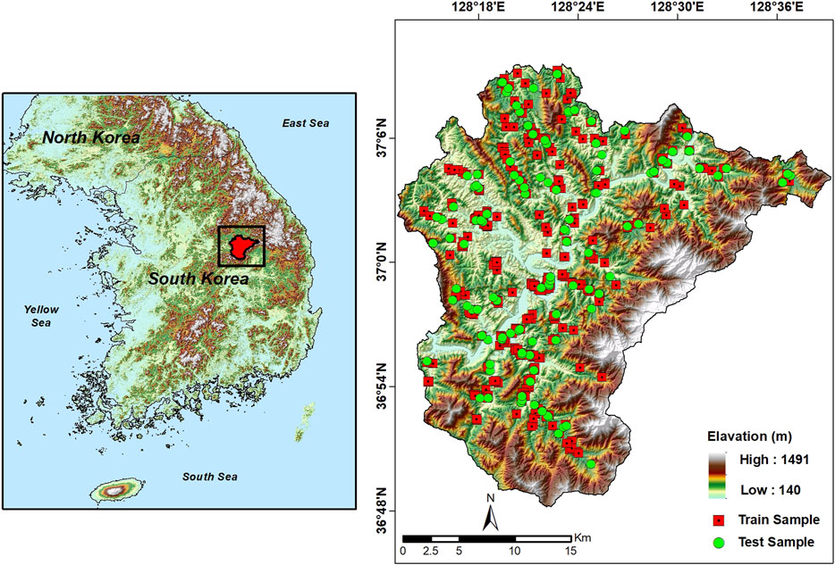
FIGURE 1. Map of the study area showing radon monitoring sites.

Danyang-gun is composed of various lithological units and strata, as well as complex and diverse geological structures. It consists of Precambrian base rock, Paleozoic sedimentary rock, Mesozoic sedimentary rock, and igneous rock (Figure 2). The Precambrian rock is located in the eastern study area and coincides with Sobaek Mountain. This rock has undergone granitization after regional metamorphism; it is divided into granitic and migmatitic gneisses (Won and Lee, 1967). The sedimentary rock includes unknown age quartzite, Paleozoic clastic sedimentary rock, and carbonate rock. The quartzite covers carbonate rock on the northwest side with an unconformity and is located at the western end of the study area. However, the sequence of formation is unclear because there is no direct contact with other formations (Won and Lee, 1967). The clastic sedimentary rock is composed of Cambrian quartzite and slate; it generally shows a strike of N30°E or N45°E. The carbonate rock is Cambrian–Ordovician and courses in the NE and NW directions (Aum et al., 2019). The NE carbonate rock consists of limestone, dolomitic limestone, dolomite, and banded limestone. The Mesozoic sedimentary rock covers this carbonate rock with a clinounconformity. This formation is mostly composed of clastic sedimentary rock such as shale, sandstone, and conglomerate; layers containing anthracite have also been identified.

FIGURE 2

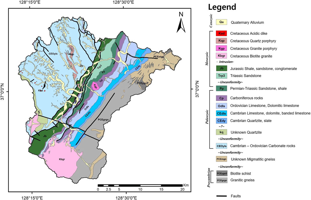
FIGURE 2. Geological map of Danyang-gun (Modified from Chwae et al. (1995)).

A fault exists in the northern part of the most recent Mesozoic formation, and carbonate rock from the NW direction is distributed to the north of the study area according to this fault. Most carbonate rock from the NW direction is composed of limestone and dolomite; several types of clastic sedimentary rock of unknown age are also present. Mesozoic rock is divided into sedimentary and igneous rock. The sedimentary rock is distributed in the NE direction, as described above. The igneous rock intruded in the Cretaceous period; it includes biotite granite, quartz porphyry, and granite porphyry. The biotite granite, which is widely distributed in the south, is in contact with sedimentary rock; this forms a contact metamorphic zone. There are faults in the NE and NW directions in the study area. The faults in the NE direction cross the center of the study area, and the geology on both sides is clearly distinguished by these faults. The faults in the NW direction cut the sedimentary formations with an NE strike in an almost perpendicular direction (Won and Lee, 1967).

2.2 Theoretical Background of the Methods

2.2.1 Long Short-Term Memory

LSTM is a deep learning algorithm with an architecture analogous to that of an artificial recurrent neural network. The LSTM is designed to capture long-term dependencies between variables; it has been developed to resolve the exploding and vanishing gradient problem of recurrent neural networks via its memory cell structure (Vu et al., 2021). A memory cell comprises a forget gate ($f_t$), an input gate ($i_t$), and an output gate ($o_t$); it regulates the flow of information entering and exiting the cell. Gates are employed to remove, maintain, or add information to the cell. The forget gate is the first filter determining whether information passes to the next time step or is discarded from the cell; it examines the current input ($x_t$) and previous hidden state ($h_{t-1}$). Subsequently, the input gate decides on the input that should be employed to update the memory; ${\tilde{C}}_t$ contains the new information. Finally, the output gate determines the information that should be regarded as output (Fang et al., 2021). This process can be expressed mathematically, as follows (Shi et al., 2021):

$Forgetgate:f_t=\sigma \left(W_f\cdot \left[h_{t-1},x_t\right]+b_f\right)(1)$

$Inputgate:\{\begin{array}{c}{i}_t=\sigma \left(W_i\cdot \left[h_{t-1},x_t\right]+b_i\right)\\ {\tilde{C}}_t=tanh\left(W_c\cdot \left[h_{t-1},x_t\right]+b_c\right)\end{array}(2)$

$Outputgate:o_t=\sigma \left(W_o\cdot \left[h_{t-1},x_t\right]+b_o\right)(3)$

where $\sigma$, $W$, and $b$ are the sigmoid function, weight matrix, and corresponding bias vector of each gate, respectively. The new memory cell is updated as follows:

$C_t=f_t\times C_{t-1}+i_t\times {\tilde{\text{C}}}_t(4)$

where $\times$ denotes the element-wise multiplication of two vectors, and $C_{t-1}$ and $C_t$ are the previous and new memory cell states, respectively (Chen et al., 2020). The hidden layer is a vector of probabilities is passed to the next time step; it is defined as follows:

$h_t=o_t\times tannh\left(C_t\right)(5)$

Finally, the output of the LSTM network at time $t$ is calculated as follows (Zhang et al., 2020):

$y_t=\sigma \left(W_y{h}_t+b_y\right)(6)$

2.2.2 Extreme Learning Machine

The ELM, a type of feed-forward neural network, has been widely used to solve regression, clustering, image processing and classification problems. Recently, the ELM has attracted considerable attention from researchers because of its high generalization performance and remarkably fast learning rate compared with traditional methods. The minimal requirement for human intervention is another advantage of the ELM approach, where most parameters can be randomly generated (Yahia et al., 2021). In particular, the ELM can adaptively determine the number of nodes in the hidden layer, randomly assign the input weights and hidden layer biases using an activation function, and obtain output layer weights through the least squares method; these abilities appreciably enhance the learning speed and generalization ability (Ding et al., 2015). For a given training dataset composed of $N$ samples $\left(x_i,t_i\right)\in R^n\times R^m\left(i=\mathrm{1,2},\dots ,N\right),$ the ELM model is defined mathematically as follows (Ding et al., 2015):

$\begin{array}{cc}{\displaystyle \sum }_{i=1}^{\tilde{N}}{\beta }_i{f}_i\left(x_j\right)={\displaystyle \sum }_{i=1}^{\tilde{N}}{\beta }_{i}f\left(a_i⊚x_j+{\mathit{b}}_i\right)={\mathit{t}}_j& j=\mathrm{1,2},\dots ,N\end{array}(7)$

where $\tilde{N}$ represents the number of hidden nodes; good generalization performance will be obtained if $\tilde{N}\ll N$. $⊚$ indicates the inner product of vectors, $f\left(x\right)$ is the non-linear activation function, and $b_i$ denotes the $i$ -th hidden node bias. Finally, $a_i$ and ${\beta }_i$ are the weight vectors, such that $a_i$ connects the input nodes to the $i$ -th hidden node and ${\beta }_i$ connects the $i$ -th hidden node to the output nodes. Equation 7 can be simply expressed as follows:

$H\beta =T(8)$

where $\beta ={\left[\begin{array}{c}{\beta }_1^T\\ {\beta }_2^T\\ ⋮\\ {\beta }_N^T\end{array}\right]}_{N\times m}$ and $T={\left[\begin{array}{c}{T}_1^T\\ t_2^T\\ ⋮\\ t_N^T\end{array}\right]}_{N\times m}$. $H$, as the hidden layer output matrix, is represented as follows:

$H\left(a_1,a_2,\dots ,a_{\tilde{N}},b_1,b_2,\dots ,b_{\tilde{N}},x_1,x_2,\dots ,x_N\right)={\left[\begin{array}{ccc}f\left(a_1⊚x_1+b_1\right)& \cdots & f\left(a_{\tilde{N}}⊚x_1+b_{\tilde{N}}\right)\\ ⋮& \ddots & ⋮\\ f\left(a_1⊚x_N+b_1\right)& \cdots & f\left(a_N⊚x_{\tilde{N}}+b_{\tilde{N}}\right)\end{array}\right]}_{N\times \tilde{N}}(9)$

In summary, the ELM stages can be described as follows:

After defining $f\left(x\right)$ and $\tilde{N}$, training is initiated, and $a_i$ and $b_i$ are randomly assigned ($i=\mathrm{1,2},\dots ,\tilde{N})$. Thereafter, $H$ is calculated according to Eq. 9. Finally, the output weight $\beta$ is calculated as follows:

$\widehat{\beta }=H^{†}T(10)$

where $H^{†}$ shows the generalized inverse of $H$, which can be computed using various methods (e.g., singular value decomposition, orthogonal projection, and iterative and orthogonalization methods) (Rao and Mitra, 1973). However, the singular value decomposition method is mostly used in ELM implementations because of the limitations of the other approaches (Liang et al., 2006).

2.2.3 Random Vector Functional Link Networks

RVFL networks represent another type of single hidden layer feed-forward neural network; these have received considerable attention because of their ability to non-iteratively adjust network weights, fast convergence, and simple network architectures. Moreover, unlike ELM networks, RVFL networks have direct connections between input and output nodes, thus preventing overfitting problems (Zhang et al., 2019). In RVFL networks, hidden-to-output and input-to-output node weights can be determined using the Moore–Penrose pseudo-inverse or ridge regression method during the training stage; other parameters (e.g., weights between the input-to-hidden node and biases) are randomly selected in the interval $[-\mathrm{1,1}]$ without iterative tuning (Cao et al., 2018; Abd Elaziz et al., 2021). An RVFL network with $l$ hidden nodes can be formulated as follows (Zhang et al., 2019):

$\begin{array}{cc}{y}_i={\displaystyle \sum }_{j=1}^l{\beta }_j{h}_j\left(x_i\right)+{\displaystyle \sum }_{j=l+1}^{l+d}{\beta }_j{x}_{ij}& i=\mathrm{1,2},\dots ,N\end{array}(11)$

where $\left(x_i,y_i\right)\in R^d\times R^c\left(i=\mathrm{1,2},\dots ,N\right)$ represents the training samples, among which $x_i$ and $y_i$ are $d$- and $c$ -dimensional input and target vectors, respectively. $h_j\left(x_i\right)$ represents the activation value for the $j$ -th hidden node, $x_{ij}$ denotes the $j$ -th attribute in the $i$ -th instance, and $\text{β}\in R^{\left(l+d\right)\times c}$ indicates the output weight matrix for the hidden nodes; these nodes can be calculated through the least squares method, as follows (Zhang et al., 2019):

$\beta ={\left(H^{T}H\right)}^{-1}{H}^{T}Y(12)$

where $H={\left[\begin{array}{ccc}{h}_1\left(x_1\right)& \cdots & h_l\left(x_1\right) \\ ⋮& \ddots & ⋮ \\ h_1\left(x_N\right)& \cdots & h_l\left(x_N\right)\end{array}\begin{array}{ccc}{x}_{11}& \dots & x_{1d}\\ ⋮& \ddots & ⋮\\ x_{N1}& \dots & x_{Nd}\end{array}\right]}_{N\times \left(l+d\right)}$.

2.3 Factor Selection

Various geological, geochemical, and topographical factors are associated with IRC values. Following a literature review and assessment of the available data, as well as application of the FR method, 10 effective factors were identified for IRC modeling (Table 1). These factors included lithology; fault density; mean soil calcium oxide (CaO), copper (Cu), lead (Pb), and ferric oxide (Fe₂O₃) concentrations; elevation; slope; valley depth; and TWI. Importantly, the FR values reflect probabilistic spatial relationships of dependent variables (IRC values, obtained from field measurements) with the various classes of each independent variable (“radon factors”). The FR values can be calculated as follows:

$FR=\frac{N_r/T_r}{N_p/T_p}(13)$

where $N_r$ is the number of training samples in each subclass of IRC effective factors, $T_r$ denotes the total number of training samples, $N_p$ is the is the number of pixels of each sub-class of the effective factor, and $T_p$ indicates the total pixels of the study area. An FR value >1 indicates a high correlation between radon level and a particular factor, an FR value <1 indicates a low correlation, and an FR value of 1 indicates a moderate correlation (Al-Abadi et al., 2016).

TABLE 1

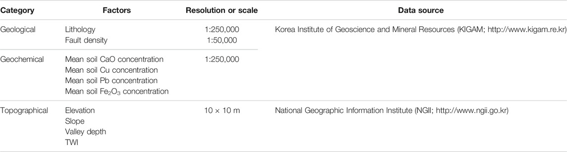
TABLE 1. Factors considered to map indoor radon levels.

To identify relationships among the included effective factors, multicollinearity analysis was performed based on the variance inflation factor ($VIF$) and tolerance ($TOL$) (Arabameri et al., 2021c). Importantly, some factors were found to exert a negative influence on the predictive capacity of the model. Such variables were removed from the model to increase its prediction accuracy (Miraki et al., 2019). The relative importance and predictive abilities of the various factors were determined using the information gain ratio ($IGR$). This is an entropy-based method that only considers variables associated with occurrence of an event (Bui et al., 2018). A higher IGR value indicates that a factor has greater impact on the model predictions (Panahi et al., 2021).

2.4 Geospatial Database of Radon Factors

Radon levels and their controlling factors vary spatially, and the selection of appropriate predictive variables is important for radon mapping accuracy. As shown in Table 1, 10 geogenic effective factors were used to model the indoor radon level. Local lithology and fault density are crucial factors affecting radon production and distribution, even in adjacent areas (Buttafuoco et al., 2010). Radon is released naturally via uranium-bearing mineral decay, such that fractures and faults provide an important route for radon migration from bedrock to the surface (Ciotoli et al., 2017). For the current study, geological and geochemical maps from the Korea Institute of Geoscience and Mineral Resources (https://www.kigam.re.kr/) were used (Figure 3). In addition to site geological characteristics, the concentrations of some chemical elements (i.e., CaO, Cu, Pb, and Fe₂O₃) remaining in minerals and soil after erosion can affect IRCs. Soil geochemistry can serve as a predictor of radon level (Ball et al., 1991; Schumann and Gundersen, 1997; Drolet et al., 2014). The effects of bedrock geochemistry on IRC are reportedly greater than those of topsoil properties, because a large portion of the topsoil tends to be removed during construction; thus, only a few centimeters remain (Appleton, 2013).

FIGURE 3

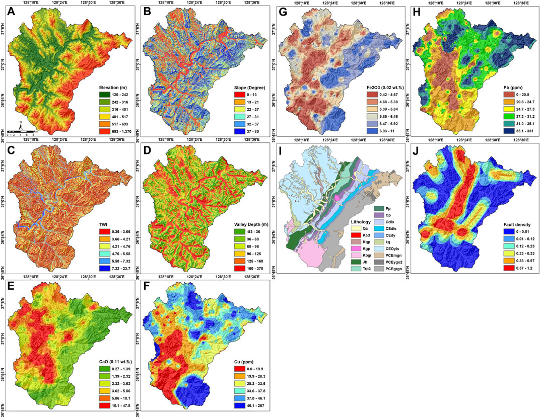
FIGURE 3. Indoor radon maps: (A) elevation, (B) slope, (C) TWI, (D) valley depth, (E) mean soil CaO concentration, (F) mean soil Cu concentration, (G) mean soil Fe₂O₃ concentration, (H) mean soil Pb concentration, (I) lithology, and (J) fault density.

In addition to geological variables, topographical factors were considered for our indoor radon potential mapping. The data were derived from a digital elevation model with a resolution of 10 m, provided by the National Geographic Information Institute (http://www.ngii.go.kr). The data were processed by SAGA software (http://www.saga-gis.org/en/index.html) to produce slope, valley depth, and TWI maps (Figure 3). In the present study, the TWI was used as a proxy of the spatial distribution of soil moisture, and was calculated as follows:

$TWI=\ln \frac{\beta }{\tan \alpha }(14)$

where $\beta$ and $\alpha$ are the cumulative catchment area in m² and slope angle in radians, respectively (Arabameri et al., 2021b). The TWI can reflect the water transmissivity and infiltration rate at a given location. Areas with low slope angles have high TWI values, while steeper areas have low TWI values (Mattivi et al., 2019). Notably, pores saturated with water trap radon in the soil and slow its transport through soil into the atmosphere (Kellenbenz and Shakya, 2021; Shahrokhi and Kovacs, 2021). However, soil moisture content can influence radon escape from mineral matter if fewer than 30% of the soil pores are filled with water; higher soil moisture content leads to a considerable reduction in radon emanation because of decreased gas permeability (Je et al., 1999). Furthermore, large valley depth values indicate areas with low elevation and gentle slopes (Figure 3). In such areas, the infiltration rate is high; the high soil wetness and fine texture lead to low permeability, in turn causing convective radon flow and slow soil gas exhalation (Wiegand, 2001).

2.5 Model Development

The generation of a radon inventory map is important for developing a machine learning-based model. In the current study, with the aim of obtaining representative samples of indoor radon levels, 1,452 dwellings were selected at random throughout the study area. Since 2008, passive IRC measurements have been conducted by National Institute of Environmental Research (NIER) using alpha-track detectors (Raduet; Radosys Ltd., Budapest, Hungary). The detectors were typically positioned in the living room, where residents spent most of their time. Each measurement period (all in winter) was 90 days in duration; the collected data were returned to NIER for analysis, and showed that the IRC value exceeded the recommended level of 148 Bqm⁻³ in 726 samples. To develop the model, samples were classified in a binary manner in terms of their IRC values. Samples with IRC >148 Bqm⁻³ were coded as 1, indicating locations with high radon levels. All remaining samples with low IRC values were coded as 0, indicating locations with low radon levels. Two classes of data (high and low radon levels) with equal numbers of samples (726) were randomly divided into training and testing subsets at the ratio of 70:30 (Kadirhodjaev et al., 2020; Panahi et al., 2021; Roy et al., 2021). The distribution of the training and testing samples is illustrated in Figure 1. To build the model, the training dataset was constructed by combining 508 samples belonging to the high and low radon level classes. Similarly, to validate the predictive accuracy of the model, the testing dataset was constructed from 218 samples that belonged to the high and low radon level classes. The training and testing datasets were then superimposed with all of the radon factors to extract their attribute characteristics. Finally, the data were transferred into MATLAB software (https://www.mathworks.com) to construct the LSTM, ELM, and RVFL models.

2.6 Model Validation

Model validation is critical to confirm the reliability of machine learning algorithms. Various statistical analysis methods are used to evaluate modeling accuracy. The area under the receiver operating characteristic curve (AUROC) is a useful quantitative parameter, where accurately detected events are plotted on the y-axis (i.e., sensitivity) against false detections on the x-axis (i.e., 1–specificity). AUROC can be constructed from both training and testing datasets, to yield success and prediction rates, respectively. The success rate curve represents model accuracy according to the locations of the samples; the prediction rate curve indicates the predictive power or generalizability of the model (Golkarian and Rahmati, 2018). The AUROC takes a value between 0 and 1, where values closer to 1 reflect better predictive ability (Park et al., 2017).The root mean square error (RMSE) and standard deviation (StD) are another statistical approaches used to assess the prediction accuracy of a model with $n$ total variables, as follows:

$RMSE=\sqrt{\frac{1}{n}{\displaystyle \sum }_{i=1}^n{\left(X_{predicted}-X_{actual}\right)}^2}(15)$

$StD=\sqrt{\frac{1}{n}{\displaystyle \sum }_{i=1}^n{\left(X_{predicted}-{\overline{X}}_{predicted}\right)}^2}(16)$

where ${\overline{X}}_{predicted}$ is the mean value of the predicted dataset, $X_{predicted}$ and $X_{actual}$ indicate the predicted and actual values of the variable, respectively. An overview of the methods used for indoor radon potential mapping is provided in Figure 4.

FIGURE 4

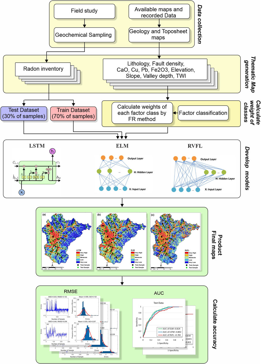
FIGURE 4. Flowchart of the method used to map indoor radon potential.

3 Results

3.1 Multicollinearity and IGR Analysis

Collinearity among effective radon factors was determined by calculating the $VIF$ and $TOL$, where $VIF>10$ and $TOL<0.1$ indicate collinearity among predictors (Arabameri et al., 2021a). As shown in Table 2, the $VIF$ and $TOL$ values of the selected factors were lower than the critical values; thus, there was no collinearity among inputs. Notably, elevation had the lowest $TOL$ (0.316) and highest $VIF$ (3.160).

TABLE 2

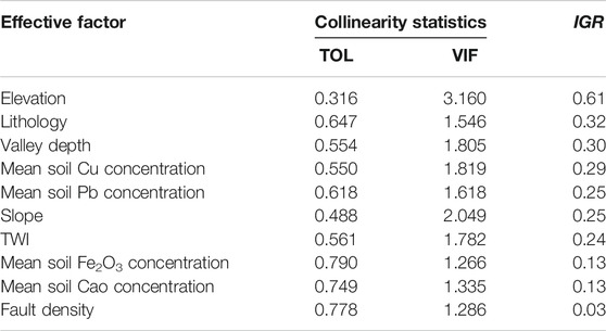
TABLE 2. Multicollinearity analysis using VIF, TOL, and IGR.

The $IGR$ method was applied to rank the predictive capabilities of the variables; the results indicated that elevation had the strongest effect on radon-prone area mapping ($IGR$ = 0.61), followed by lithology (0.32), valley depth (0.30), and mean soil Cu concentration (0.29). In fact, all factors with $IGR>0$ had predictive power (Table 2).

3.2 Assessment of the Contributions of Each Factor to Model Performance

Various geogenic factors can affect radon levels; this can be quantified through statistical modeling, such as the FR method. Stronger correlations are indicated by higher FR values, while $FR<1$ indicates a weak relationship between a given predictor and the IRC value. As shown in Table 3, 10 variables were used to predict areas with potentially dangerous radon levels. The results implied that an elevation of 120–242 m (FR = 3.29) had the greatest influence on the IRC. Importantly, approximately 80% of Danyang-gun is mountainous, with a shallow soil profile that mostly contains coarse fragments. This promotes soil permeability and movement of radon gas within the soil (Hauri et al., 2012). In contrast, soil gas accumulation in lowlands is high; thus, it can easily infiltrate indoor environments via the soil through openings and cracks in basement foundations. Analysis of the FR values for the slope factor showed that the highest value (2.41) was associated with the class of 0–13.5°. This finding implies that the IRC decreases in sloped areas because the released radon is rapidly diluted in outdoor air (Appleton, 2013). In terms of valley depth and TWI, the highest FR values were found in the sixth (161–370 m) and fifth (5.59–7.32) classes, respectively. These factors reflect the effects of hydrological variables (e.g., rainfall-runoff and infiltration rates) and soil moisture content on soil gas exhalation capacity; this capacity is generally diminished when soil wetness is increased (Sasaki et al., 2004; Raduła et al., 2018). Analysis of the relationship between the radon emanation rate and presence of specific uranium- and radium-containing minerals (i.e., in the host rock and remaining soils after weathering) showed that the highest values of FR were 1.47, 1.59, 1.76, and 1.48 for mean soil CaO, Cu, Pb, and Fe₂O₃ concentrations, respectively. For all factors, the FR values were >1, indicating strong correlations with radon levels at the monitoring sites. Furthermore, radon levels were high in areas where the fault density varied between 0.58 and 1.2 (FR = 2.32). Notably, fault systems located in fracture zones provide a route for radon to migrate upward from deeper sources (Han et al., 2006). Finally, in terms of lithology, the FR analysis yielded higher values, of 200.65, 32.74, and 13.71, for Cretaceous acidic dike (Kad), Cretaceous quartz porphyry (Kqp), and Cambrian quartzite and slate (CEdy) units, respectively. Generally, sedimentary, igneous, and metamorphic rocks contain variable amounts of uranium and radium, depending on the rock formation processes (Pasculli et al., 2014).

TABLE 3

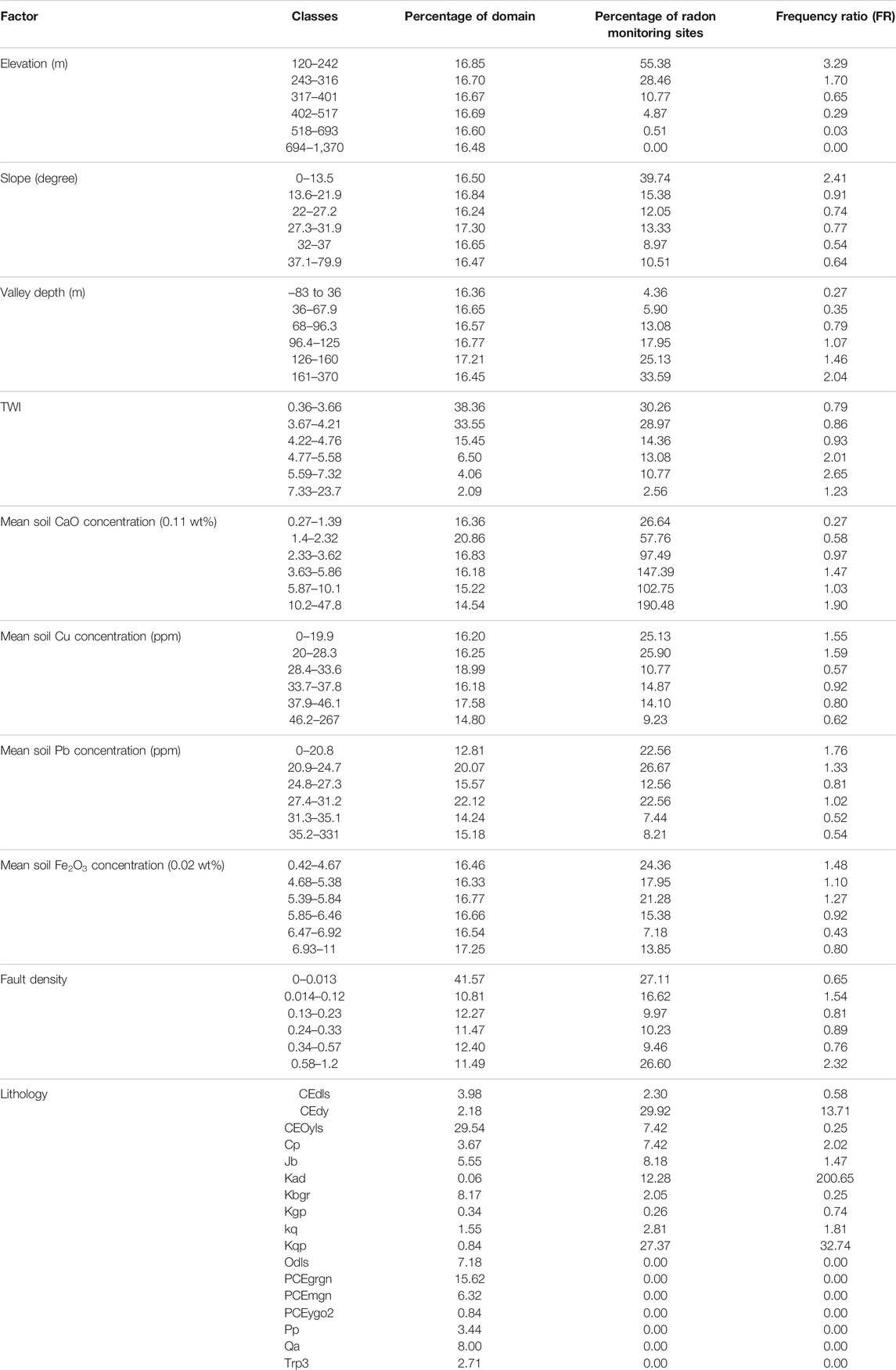
TABLE 3. Spatial relationships of predictor variables with the IRC values, determined through FR analysis.

3.3 Radon Potential Mapping

The maps generated using the LSTM, ELM, and RVFL algorithms are shown in Figure 5. The maps included five classes of radon-prone areas (very low, low, moderate, high, and very high), based on the quantile method (Khosravi et al., 2018). The percentage area of each class on each map is shown in Figure 6. The ELM model was the most accurate; it categorized 19.62, 20.64, 19.84, 20.01, and 19.88% of the study area into the very low, low, moderate, high, and very high classes. As depicted in Figure 5, high radon levels were observed in central and southwestern parts of the study area due to the distribution of sedimentary rock and unconsolidated deposits such as carbonate, shale, sandstone, conglomerate, limestone, and dolomite, all of which are rich in uranium and organic materials. These findings were consistent with the results of previous studies (Cho et al., 2015; Hwang et al., 2017; Kim and Ha, 2018; Park et al., 2019).

FIGURE 5

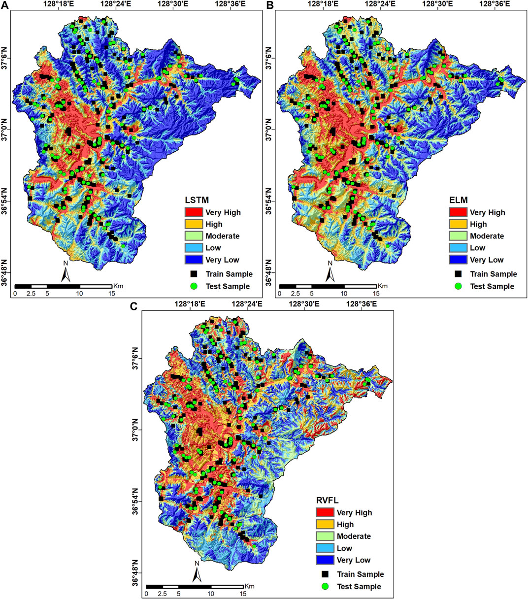
FIGURE 5. Radon potential maps derived from the (A) LSTM, (B) ELM, and (C) RVFL models.

FIGURE 6

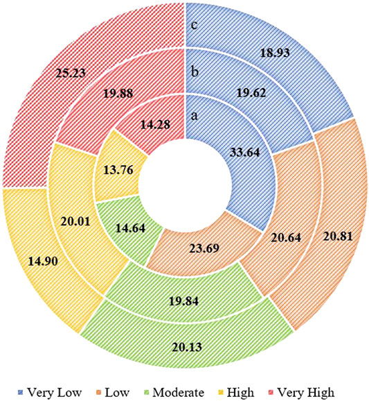
FIGURE 6. Percentage areas of the different radon potential classes for the (a) LSTM, (b) ELM, and (c) RVFL models.

The reliability of the results was checked using the FR method, which revealed that most of the samples with high radon levels were from the very high and high radon potential areas. Thus, the models exhibited satisfactory performance in terms of study area classification. The AUROC values were calculated to quantitatively evaluate the predictive accuracy of each model. The AUROC values for the success rate curve analysis of the LSTM, ELM, and RVFL models were 0.81, 0.83, and 0.82, respectively. The AUROC value for the prediction rate curve analysis was 0.82 for the ELM model; the LSTM and RVFL models had lower values of 0.80 and 0.78, respectively (Figure 7). The RMSE values exhibited a similar pattern. As shown in Figure 8, analysis based on training data showed that the RMSE was lowest for the ELM model (0.152); the LSTM and RVFL models exhibited higher RMSEs of 0.163 and 0.182, respectively. Further analysis based on the testing data showed that the RMSEs of the ELM, LSTM, and RVFL models were 0.209, 0.232, and 0.0286, respectively. The standard deviation (StD) values for the ELM model (0.152 and 0.207) were lower than those for the LSTM and RVFL models, during both the training and validation phases. In summary, by comparison of the AUROC, RMSE, and StD values calculated using the training and testing datasets, all of the evaluated models had acceptable performance in terms of classifying radon-prone areas; however, the ELM model was slightly superior to the two other models.

FIGURE 7

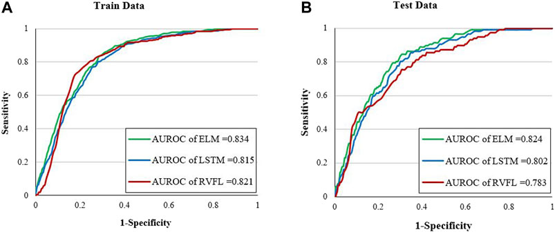
FIGURE 7. (A) Success rate curve and (B) prediction rate curve AUROC results.

FIGURE 8

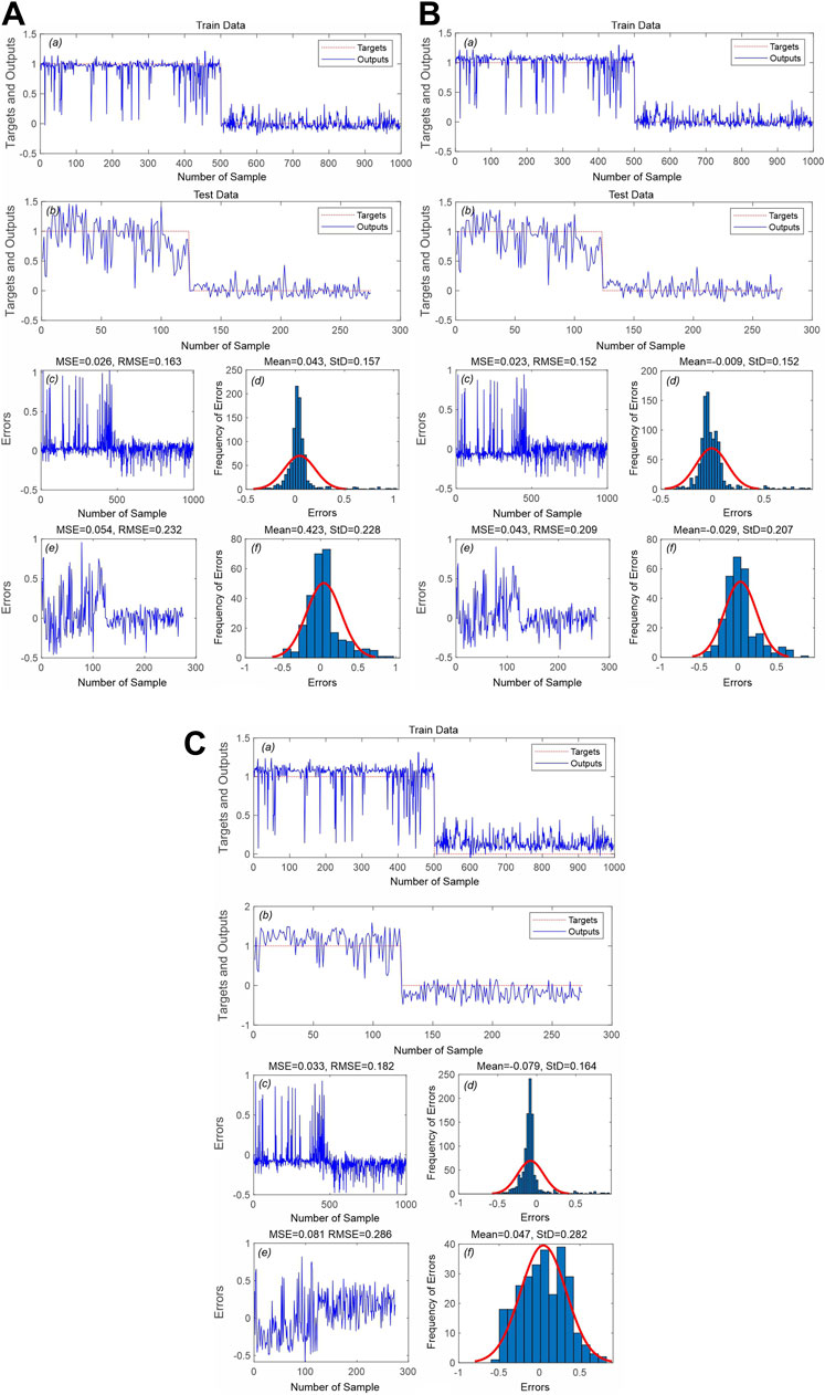
FIGURE 8. Assessment of model performance: (A) LSTM, (B) ELM, and (C) RVFL. (a) Targets and outputs for the training dataset; (b) targets and outputs for the testing dataset; (c) MSE and RMSE for the training dataset; (d) frequency of errors for the training dataset; (e) MSE and RMSE for the testing dataset; (f) frequency of errors for the testing dataset.

4 Discussion

As a subclass of data-driven methods, machine learning algorithms have attracted attentions in geospatial studies because of their robust performance in modelling nonlinear problems. The present study was conducted to determine the effects of geogenic factors on radon levels in residential environments, and to identify areas of high radon risk using machine learning methods. To fulfill these aims, IRCs were measured during field surveys of 1,452 dwellings. Notably, IRCs exceeded the threshold value (148 Bqm⁻³) in 726 locations; they varied from 148.7 to 1,775.1 Bqm⁻³, with a mean value of 346.9 Bqm⁻³. This study demonstrated that the geological and topographical properties of a given site are the fundamental drivers of IRC spatial variability. Higher IRC values were observed in the central and southwestern parts of the study area (Figure 5), where the dominant lithology is limestone; the higher fault density in that region facilitates radon migration from bedrock to the surface. These results were consistent with the findings of Park et al. (2019), who reported that the mean IRCs were higher in Danyang than other counties in South Korea; the high values in that study were attributable to coal-bearing formations in the Daedong system and limestone intercalation in the Pyeongan system. Additionally, more than 200 limestone caves are present in Danyang; radon gas can easily accumulate in the holes within limestone areas and moves to the surface through faults and fractures. Therefore, lithology can be considered as a key predictor in defining geogenic radon-prone areas, in line with former studies including Przylibski et al. (2011) and Cho et al. (2015), who revealed the relationship between radon levels and variability of lithological units in the study area. In addition, Kim et al. (2011) pointed out that the high IRC values were correlated with the concentration of radionuclides in the surface soil and granitic rocks distribution in South Korea.

Furthermore, elevation had a greater effect on the IRC values in the present study than lithology, according to the $IGR$ analysis. In highland areas with steep slopes, soil has coarser fractions; consequently, it also has high permeability, such that radon gas emitted from rocks and surficial soil can easily migrate to the atmosphere and rapidly disperse in open air. Conversely, in areas of low elevation with gentle slopes, where most of the residential areas are located, indoor radon levels are high because there are no mitigation activities (Cinelli et al., 2015). Oliver and Khayrat (2001) showed the inverse relationship between radon concentrations and elevation. It perfectly overlaps the findings of Siaway et al. (2010), Mose et al. (2010), and Cho et al. (2015), who concluded that in highlands with steep slopes, indoor radon levels may be reduced because of high soil permeability. The presence of coarser soil with limited moisture leads to less soil accumulation of radon beneath buildings because of more rapid dilution of radon emanating from host rocks in the outdoor air.

Accurate determination of the geographical distribution of IRCs and prediction of radon priority areas can inform construction regulations and promote more cost-effective radon policies. We used three machine learning algorithms (i.e., LSTM, ELM, and RVFL) to map areas of high radon risk. The AUROC, RMSE, and StD values indicated that the ELM was superior to the LSTM and RVFL, in terms of predictive accuracy, during both the training and validation phases. The main advantage of the ELM method is that only the hidden layer weights require adjustment; therefore, it has better generalizability and is less computational complex, especially for large-scale samples (Liu et al., 2012; Fernández et al., 2019). The present study supports the findings of Lian et al. (2014), Huang et al. (2017), Yadav et al. (2017), and Anupam and Pani (2020), who stated the efficiency and applicability of the ELM algorithm to generating more accurate predictive models in various fields of study such as landslide displacement prediction, landslide susceptibility mapping, groundwater level prediction, and flood forecasting, respectively. However, the suitability of the ELM model for identifying the radon-affected areas has not been reported in the literature.

5 Conclusion

IRCs were measured in 1,425 randomly selected dwellings in Danyang-gun, South Korea, to facilitate indoor radon potential mapping using LSTM, ELM, and RVFL machine learning algorithms. The results showed that the ELM method had the best prediction performance; approximately 40% of the study area was located within very high and high-risk radon potential zones. Elevation was the strongest predictor of radon-prone areas, followed by lithology and valley depth.

Uranium and thorium in soil and rocks are the main sources of variability in IRC values, and more than 80% of the ionizing radiation to which humans are exposed is of natural origin (Pantelić et al., 2019). However, in this study the distribution of radon in indoor environments could not be reliably estimated solely on the basis of geogenic factors. In addition to the characteristics of the underlying soils and rocks, building materials, ventilation systems and resident lifestyles can substantially affect indoor radon levels. Nevertheless, the results of the present study should facilitate identification of high radon areas, and thus allow the negative effects of natural radon on human health to be reduced (through regular monitoring of existing houses and the imposition of restrictions on the construction of new structures in affected areas). An accurate indoor radon map is important for more efficient future surveys.

Data Availability Statement

The original contributions presented in the study are included in the article/supplementary material, further inquiries can be directed to the corresponding authors.

Author Contributions

FR: Conceptualization, writing–original draft, writing-review and editing, software, formal analysis, data curation, visualization; SK: Writing–original draft; MA: Writing–original draft; MP: Methodology, validation, writing-review and editing, visualization; HK: Writing–original draft; SK: Resources, review and editing; JL: Resources, review and editing; JL: Resources, review and editing; JY: Resources, review and editing; and SL: Supervision, Funding acquisition, project administration.

Conflict of Interest

The authors declare that the research was conducted in the absence of any commercial or financial relationships that could be construed as a potential conflict of interest.

Publisher’s Note

All claims expressed in this article are solely those of the authors and do not necessarily represent those of their affiliated organizations, or those of the publisher, the editors and the reviewers. Any product that may be evaluated in this article, or claim that may be made by its manufacturer, is not guaranteed or endorsed by the publisher.

Acknowledgments

This research was supported by the Basic Research Project of the Korea Institute of Geoscience and Mineral Resources (KIGAM) and Project of Environmental Business Big Data Platform and Center Construction funded by the Ministry of Science and ICT. Furthermore, this work was supported by a grant from the National Institute of Environmental Research (NIER), funded by the Ministry of Environment (MOE) of the Republic of Korea (NIER-2017-03-01-017).

References

Abd Elaziz, M., Senthilraja, S., Zayed, M. E., Elsheikh, A. H., Mostafa, R. R., and Lu, S. (2021). A New Random Vector Functional Link Integrated with Mayfly Optimization Algorithm for Performance Prediction of Solar Photovoltaic thermal Collector Combined with Electrolytic Hydrogen Production System. Appl. Therm. Eng. 193, 117055. doi:10.1016/j.applthermaleng.2021.117055

CrossRef Full Text | Google Scholar

Al-Abadi, A. M., Al-Temmeme, A. A., and Al-Ghanimy, M. A. (2016). A GIS-Based Combining of Frequency Ratio and index of Entropy Approaches for Mapping Groundwater Availability Zones at Badra-Al Al-Gharbi-Teeb Areas, Iraq. Sustain. Water Resour. Manag. 2, 265–283. doi:10.1007/s40899-016-0056-5

CrossRef Full Text | Google Scholar

Al-Fugara, A. k., Pourghasemi, H. R., Al-Shabeeb, A. R., Habib, M., Al-Adamat, R., Al-Amoush, H., et al. (2020). A Comparison of Machine Learning Models for the Mapping of Groundwater Spring Potential. Environ. Earth Sci. 79, 206. doi:10.1007/s12665-020-08944-1

CrossRef Full Text | Google Scholar

Anupam, S., and Pani, P. (2020). Flood Forecasting Using a Hybrid Extreme Learning Machine-Particle Swarm Optimization Algorithm (ELM-PSO) Model. Model. Earth Syst. Environ. 6, 341–347. doi:10.1007/s40808-019-00682-z

CrossRef Full Text | Google Scholar

Appleton, J. D. (2013). “Radon in Air and Water,” in Essentials of Medical Geology. (Dordrecht: Springer Netherlands), 239–277. doi:10.1007/978-94-007-4375-5_11

CrossRef Full Text | Google Scholar

Arabameri, A., Chandra Pal, S., Costache, R., Saha, A., Rezaie, F., Seyed Danesh, A., et al. (2021a). Prediction of Gully Erosion Susceptibility Mapping Using Novel Ensemble Machine Learning Algorithms. Geomatics, Nat. Hazards Risk 12, 469–498. doi:10.1080/19475705.2021.1880977

CrossRef Full Text | Google Scholar

Arabameri, A., Lee, S., Rezaie, F., Chandra Pal, S., Asadi Nalivan, O., Saha, A., et al. (2021b). Performance Evaluation of GIS-Based Novel Ensemble Approaches for Land Subsidence Susceptibility Mapping. Front. Earth Sci. 9, 663678. doi:10.3389/feart.2021.663678

CrossRef Full Text | Google Scholar

Arabameri, A., Pal, S. C., Rezaie, F., Nalivan, O. A., Chowdhuri, I., Saha, A., et al. (2021c). Modeling Groundwater Potential Using Novel GIS-Based Machine-Learning Ensemble Techniques. J. Hydrol. Reg. Stud. 36, 100848. doi:10.1016/j.ejrh.2021.100848

CrossRef Full Text | Google Scholar

Aum, H. W., Kim, Y., Cheong, W., and Hau, B. V. (2019). SHRIMP Zircon U-Pb Age and Geochemistry of Granites in the Gudambong-Sainam Geosites, Danyang Geopark. J. Petrol. Soc. Korea 28, 143–156. doi:10.7854/JPSK.2019.28.2.143

CrossRef Full Text | Google Scholar

Ball, T. K., Cameron, D. G., Colman, T. B., and Roberts, P. D. (1991). Behaviour of Radon in the Geological Environment: A Review. Q. J. Eng. Geology. Hydrogeol. 24, 169–182. doi:10.1144/GSL.QJEG.1991.024.02.01

CrossRef Full Text | Google Scholar

Bossew, P., Cinelli, G., Ciotoli, G., Crowley, Q. G., de Cort, M., Elío Medina, J., et al. (2020). Development of a Geogenic Radon Hazard Index-Concept, History, Experiences. Int. J. Environ. Res. Public Health 17, 4134–4224. doi:10.3390/ijerph17114134

PubMed Abstract | CrossRef Full Text | Google Scholar

Tien Bui, D., Shahabi, H., Shirzadi, A., Chapi, K., Hoang, N.-D., Pham, B., et al. (2018). A Novel Integrated Approach of Relevance Vector Machine Optimized by Imperialist Competitive Algorithm for Spatial Modeling of Shallow Landslides. Remote Sens. 10, 1538. doi:10.3390/rs10101538

CrossRef Full Text | Google Scholar

Buttafuoco, G., Tallarico, A., Falcone, G., and Guagliardi, I. (2010). A Geostatistical Approach for Mapping and Uncertainty Assessment of Geogenic Radon Gas in Soil in an Area of Southern Italy. Environ. Earth Sci. 61, 491–505. doi:10.1007/s12665-009-0360-6

CrossRef Full Text | Google Scholar

Cao, W., Wang, X., Ming, Z., and Gao, J. (2018). A Review on Neural Networks with Random Weights. Neurocomputing 275, 278–287. doi:10.1016/j.neucom.2017.08.040

CrossRef Full Text | Google Scholar

Cerqueiro-Pequeño, J., Comesaña-Campos, A., Casal-Guisande, M., and Bouza-Rodríguez, J.-B. (2020). Design and Development of a New Methodology Based on Expert Systems Applied to the Prevention of Indoor Radon Gas Exposition Risks. Int. J. Environ. Res. Public Health 18, 269. doi:10.3390/ijerph18010269

CrossRef Full Text | Google Scholar

Chen, X., He, J., Wu, X., Yan, W., and Wei, W. (2020). Sleep Staging by Bidirectional Long Short-Term Memory Convolution Neural Network. Future Generation Comput. Syst. 109, 188–196. doi:10.1016/j.future.2020.03.019

CrossRef Full Text | Google Scholar

Cho, B.-W., Choo, C. O., Kim, M. S., Hwang, J., Yun, U., and Lee, S. (2015). Spatial Relationships between Radon and Topographical, Geological, and Geochemical Factors and Their Relevance in All of South Korea. Environ. Earth Sci. 74, 5155–5168. doi:10.1007/s12665-015-4526-0

CrossRef Full Text | Google Scholar

Chwae, U. C., Kim, K. B., Hong, S. H., Lee, B. J., Hwang, J. H., Park, K. H., et al. (1995). Geological Map of Korea (1:1,000,000). Daejeon, South Korea: Korea Institute of Geoscience and Mineral Resources.

Cinelli, G., Tositti, L., Capaccioni, B., Brattich, E., and Mostacci, D. (2015). Soil Gas Radon Assessment and Development of a Radon Risk Map in Bolsena, Central Italy. Environ. Geochem. Health 37, 305–319. doi:10.1007/s10653-014-9649-9

PubMed Abstract | CrossRef Full Text | Google Scholar

Ciotoli, G., Voltaggio, M., Tuccimei, P., Soligo, M., Pasculli, A., Beaubien, S. E., et al. (2017). Geographically Weighted Regression and Geostatistical Techniques to Construct the Geogenic Radon Potential Map of the Lazio Region: A Methodological Proposal for the European Atlas of Natural Radiation. J. Environ. Radioact. 166, 355–375. doi:10.1016/j.jenvrad.2016.05.010

PubMed Abstract | CrossRef Full Text | Google Scholar

Ciotoli, G., Procesi, M., Finoia, M., Bossew, P., Cinelli, G., Tollefsen, T., et al. (2020). “Spatial Multicriteria Decision Analysis (SMCDA) for the Construction of the European Geogenic Radon Migration Map”, in 22nd EGU General Assembly, May 4–8, 2020, 7350. doi:10.5194/egusphere-egu2020-7350

CrossRef Full Text | Google Scholar

Cogliano, V. J., Baan, R., Straif, K., Grosse, Y., Lauby-Secretan, B., El Ghissassi, F., et al. (2011). Preventable Exposures Associated with Human Cancers. J. Natl. Cancer Inst. 103, 1827–1839. doi:10.1093/jnci/djr483

CrossRef Full Text | Google Scholar

Diego, O., Halim Essam, H., and Salvador, H. (2021). “Metaheuristics in Machine Learning: Theory and Applications,” in Studies in Computational Intelligence. Editors D. Oliva, E. H. Houssein, and S. Hinojosa. 1st Edn. (Cham: Springer International Publishing). doi:10.1007/978-3-030-70542-8

CrossRef Full Text | Google Scholar

Ding, S., Zhao, H., Zhang, Y., Xu, X., and Nie, R. (2015). Extreme Learning Machine: Algorithm, Theory and Applications. Artif. Intell. Rev. 44, 103–115. doi:10.1007/s10462-013-9405-z

CrossRef Full Text | Google Scholar

Djamil, B. (2016). Indoor Radon Mitigation in South Korea. Int. J. Appl. Eng. Res. 11, 8521–8523. doi:10.52049/gemakampus.v11i1.18

CrossRef Full Text | Google Scholar

Drolet, J.-P., Martel, R., Poulin, P., and Dessau, J.-C. (2014). Methodology Developed to Make the Quebec Indoor Radon Potential Map. Sci. Total Environ. 473-474, 372–380. doi:10.1016/j.scitotenv.2013.12.039

PubMed Abstract | CrossRef Full Text | Google Scholar

Dubois, G. (2005). An Overview of Radon Surveys in Europe. Available at: internal-pdf://84.21.186.44/2005_EUR_RADON_MAPPING.pdf.

Google Scholar

Duong, V.-H., Ly, H.-B., Trinh, D. H., Nguyen, T. S., and Pham, B. T. (2021). Development of Artificial Neural Network for Prediction of Radon Dispersion Released from Sinquyen Mine, Vietnam. Environ. Pollut. 282, 116973. doi:10.1016/j.envpol.2021.116973

PubMed Abstract | CrossRef Full Text | Google Scholar

Fang, Z., Wang, Y., Peng, L., and Hong, H. (2021). Predicting Flood Susceptibility Using LSTM Neural Networks. J. Hydrol. 594, 125734. doi:10.1016/j.jhydrol.2020.125734

CrossRef Full Text | Google Scholar

Fernández, C., Salinas, L., and Torres, C. E. (2019). A Meta Extreme Learning Machine Method for Forecasting Financial Time Series. Appl. Intell. 49, 532–554. doi:10.1007/s10489-018-1282-3

CrossRef Full Text | Google Scholar

Giustini, F., Procesi, M., Finoia, M., Sassi, R., Mazzoli, C., and Ciotoli, G. (2021). “Mapping the Geogenic Radon Hazard Index of Italy,” in 23rd EGU General Assembly, April 19–30, 2021. doi:10.5194/egusphere-egu21-7343

CrossRef Full Text | Google Scholar

Golkarian, A., and Rahmati, O. (2018). Use of a Maximum Entropy Model to Identify the Key Factors that Influence Groundwater Availability on the Gonabad Plain, Iran. Environ. Earth Sci. 77, 369. doi:10.1007/s12665-018-7551-y

CrossRef Full Text | Google Scholar

Han, Y. L., Tom Kuo, M. C., Fan, K. C., Chiang, C. J., and Lee, Y. P. (2006). Radon Distribution in Groundwater of Taiwan. Hydrogeol. J. 14, 173–179. doi:10.1007/s10040-004-0384-7

CrossRef Full Text | Google Scholar

Hauri, D. D., Huss, A., Zimmermann, F., Kuehni, C. E., and Röösli, M. (2012). A Prediction Model for Assessing Residential Radon Concentration in Switzerland. J. Environ. Radioact. 112, 83–89. doi:10.1016/j.jenvrad.2012.03.014

CrossRef Full Text | Google Scholar

Huang, F., Yin, K., Huang, J., Gui, L., and Wang, P. (2017). Landslide Susceptibility Mapping Based on Self-Organizing-Map Network and Extreme Learning Machine. Eng. Geol. 223, 11–22. doi:10.1016/j.enggeo.2017.04.013

CrossRef Full Text | Google Scholar

Hwang, J., Kim, T., Kim, H., Cho, B., and Lee, S. (2017). Predictive Radon Potential Mapping in Groundwater: A Case Study in Yongin, Korea. Environ. Earth Sci. 76, 515. doi:10.1007/s12665-017-6838-8

CrossRef Full Text | Google Scholar

Ivanova, K., Stojanovska, Z., Kunovska, B., Chobanova, N., Badulin, V., and Benderev, A. (2019). Analysis of the Spatial Variation of Indoor Radon Concentrations (National Survey in Bulgaria). Environ. Sci. Pollut. Res. 26, 6971–6979. doi:10.1007/s11356-019-04163-9

PubMed Abstract | CrossRef Full Text | Google Scholar

Je, H. K., Kang, C., and Chon, H. T. (1999). A Preliminary Study on Soil-Gas Radon Geochemistry According to Different Bedrock Geology in Korea. Environ. Geochem. Health 21, 117–131. doi:10.1023/A:1006613016217

CrossRef Full Text | Google Scholar

Kadirhodjaev, A., Rezaie, F., Lee, M. J., and Lee, S. (2020). Landslide Susceptibility Assessment Using an Optimized Group Method of Data Handling Model. ISPRS Int. J. Geo-Information 9. doi:10.3390/ijgi9100566

CrossRef Full Text | Google Scholar

Kellenbenz, K. R., and Shakya, K. M. (2021). Spatial and Temporal Variations in Indoor Radon Concentrations in Pennsylvania, USA from 1988 to 2018. J. Environ. Radioact. 233, 106594. doi:10.1016/j.jenvrad.2021.106594

CrossRef Full Text | Google Scholar

Khosravi, K., Panahi, M., and Tien Bui, D. (2018). Spatial Prediction of Groundwater Spring Potential Mapping Based on an Adaptive Neuro-Fuzzy Inference System and Metaheuristic Optimization. Hydrol. Earth Syst. Sci. 22, 4771–4792. doi:10.5194/hess-22-4771-2018

CrossRef Full Text | Google Scholar

Kim, J.-H., and Ha, M. (2018). The Disease Burden of Lung Cancer Attributable to Residential Radon Exposure in Korean Homes. J. Korean Med. Sci. 33, e223. doi:10.3346/jkms.2018.33.e223

PubMed Abstract | CrossRef Full Text | Google Scholar

Kim, Y., Chang, B.-U., Park, H.-M., Kim, C.-K., and Tokonami, S. (2011). National Radon Survey in Korea. Radiat. Prot. Dosimetry 146, 6–10. doi:10.1093/rpd/ncr094

PubMed Abstract | CrossRef Full Text | Google Scholar

Kim, S.-H., Koh, S.-B., Lee, C.-M., Kim, C., and Kang, D. R. (2018). Indoor Radon and Lung Cancer: Estimation of Attributable Risk, Disease burden, and Effects of Mitigation. Yonsei Med. J. 59, 1123–1130. doi:10.3349/ymj.2018.59.9.1123

PubMed Abstract | CrossRef Full Text | Google Scholar

KMA (2021). Korea Meteorological Administration (KMA). Available at: https://www.weather.go.kr (Accessed September 15, 2021).

Google Scholar

Lee, H. A., Lee, W. K., Lim, D., Park, S. H., Baik, S. J., Kong, K. A., et al. (2015). Risks of Lung Cancer Due to Radon Exposure Among the Regions of Korea. J. Korean Med. Sci. 30, 542–548. doi:10.3346/jkms.2015.30.5.542

PubMed Abstract | CrossRef Full Text | Google Scholar

Li, X., Peng, L., Hu, Y., Shao, J., and Chi, T. (2016). Deep Learning Architecture for Air Quality Predictions. Environ. Sci. Pollut. Res. 23, 22408–22417. doi:10.1007/s11356-016-7812-9

PubMed Abstract | CrossRef Full Text | Google Scholar

Lian, C., Zeng, Z., Yao, W., and Tang, H. (2014). Ensemble of Extreme Learning Machine for Landslide Displacement Prediction Based on Time Series Analysis. Neural Comput. Applic 24, 99–107. doi:10.1007/s00521-013-1446-3

CrossRef Full Text | Google Scholar

Nan-Ying Liang, N. Y., Guang-Bin Huang, G. B., Saratchandran, P., and Sundararajan, N. (2006). A Fast and Accurate Online Sequential Learning Algorithm for Feedforward Networks. IEEE Trans. Neural Netw. 17, 1411–1423. doi:10.1109/TNN.2006.880583

PubMed Abstract | CrossRef Full Text | Google Scholar

Liu, X., Gao, C., and Li, P. (2012). A Comparative Analysis of Support Vector Machines and Extreme Learning Machines. Neural Netw. 33, 58–66. doi:10.1016/j.neunet.2012.04.002

PubMed Abstract | CrossRef Full Text | Google Scholar

Liu, B., Zhang, L., Wang, Q., and Chen, J. (2021). A Novel Method for Regional NO2 Concentration Prediction Using Discrete Wavelet Transform and an LSTM Network. Comput. Intell. Neurosci. 2021, 1–14. doi:10.1155/2021/6631614

CrossRef Full Text | Google Scholar

Martínez, R. G., Kotsarenko, A., Enriquez, R. P., Abeyro, J. A. L. C., Koshevaya, S., and Noreña, J. E. O. (2014). Influence of Geological Factor on Indoor Radon Concentrations in Dwelling of Querétaro, México. México. Open J. Geol. 04, 627–635. doi:10.4236/ojg.2014.412047

CrossRef Full Text | Google Scholar

Mattivi, P., Franci, F., Lambertini, A., and Bitelli, G. (2019). TWI Computation: A Comparison of Different Open Source GISs. Open Geospatial Data, Softw. Stand. 4, 6. doi:10.1186/s40965-019-0066-y

CrossRef Full Text | Google Scholar

Miraki, S., Zanganeh, S. H., Chapi, K., Singh, V. P., Shirzadi, A., Shahabi, H., et al. (2019). Mapping Groundwater Potential Using a Novel Hybrid Intelligence Approach. Water Resour. Manage. 33, 281–302. doi:10.1007/s11269-018-2102-6

CrossRef Full Text | Google Scholar

Mose, D. G., Siaway, G., Metcalf, J., Mose, D. G., and Siaway, G. (2010). Geographic Information System Application to the Problem of Predicting Indoor Radon Concentrations. Int. J. Soil Sediment. Water 3, 3. Available at: https://scholarworks.umass.edu/intljssw/vol3/iss2/3/.

Google Scholar

Oliver, M. A., and Khayrat, A. L. (2001). A Geostatistical Investigation of the Spatial Variation of Radon in Soil. Comput. Geosci. 27, 939–957. doi:10.1016/S0098-3004(00)00133-3

CrossRef Full Text | Google Scholar

Pásztor, L., Szabó, K. Z., Szatmári, G., Laborczi, A., and Horváth, Á. (2016). Mapping Geogenic Radon Potential by Regression Kriging. Sci. Total Environ. 544, 883–891. doi:10.1016/j.scitotenv.2015.11.175

PubMed Abstract | CrossRef Full Text | Google Scholar

Panahi, M., Dodangeh, E., Rezaie, F., Khosravi, K., Van Le, H., Lee, M.-J., et al. (2021). Flood Spatial Prediction Modeling Using a Hybrid of Meta-Optimization and Support Vector Regression Modeling. CATENA 199, 105114. doi:10.1016/j.catena.2020.105114

CrossRef Full Text | Google Scholar

Pantelić, G., Čeliković, I., Živanović, M., Vukanac, I., Nikolić, J. K., Cinelli, G., et al. (2019). Qualitative Overview of Indoor Radon Surveys in Europe. J. Environ. Radioact. 204, 163–174. doi:10.1016/j.jenvrad.2019.04.010

CrossRef Full Text | Google Scholar

Park, S., Hamm, S.-Y., Jeon, H.-T., and Kim, J. (2017). Evaluation of Logistic Regression and Multivariate Adaptive Regression Spline Models for Groundwater Potential Mapping Using R and GIS. Sustainability 9, 1157. doi:10.3390/su9071157

CrossRef Full Text | Google Scholar

Park, T. H., Kang, D. R., Park, S. H., Yoon, D. K., and Lee, C. M. (2018). Indoor Radon Concentration in Korea Residential Environments. Environ. Sci. Pollut. Res. 25, 12678–12685. doi:10.1007/s11356-018-1531-3

PubMed Abstract | CrossRef Full Text | Google Scholar

Park, N.-W., Kim, Y., Chang, B.-U., and Kwak, G.-H. (2019). County-Level Indoor Radon Concentration Mapping and Uncertainty Assessment in South Korea Using Geostatistical Simulation and Environmental Factors. J. Environ. Radioact. 208–209, 106044. doi:10.1016/j.jenvrad.2019.106044

CrossRef Full Text | Google Scholar

Pasculli, A., Palermi, S., Sarra, A., Piacentini, T., and Miccadei, E. (2014). A Modelling Methodology for the Analysis of Radon Potential Based on Environmental Geology and Geographically Weighted Regression. Environ. Model. Softw. 54, 165–181. doi:10.1016/j.envsoft.2014.01.006

CrossRef Full Text | Google Scholar

Pegoretti, S., and Verdi, L. (2009). Machine Learning for the Analysis of Indoor Radon Distribution, Compared with Ordinary Kriging. Radiat. Prot. Dosimetry 137, 324–328. doi:10.1093/rpd/ncp254

PubMed Abstract | CrossRef Full Text | Google Scholar

Petermann, E., Meyer, H., Nussbaum, M., and Bossew, P. (2021). Mapping the Geogenic Radon Potential for Germany by Machine Learning. Sci. Total Environ. 754, 142291. doi:10.1016/j.scitotenv.2020.142291

PubMed Abstract | CrossRef Full Text | Google Scholar

Phong Thu, H. N., Van Thang, N., and Hao, L. C. (2020). The Effects of Some Soil Characteristics on Radon Emanation and Diffusion. J. Environ. Radioact. 216, 106189. doi:10.1016/j.jenvrad.2020.106189

CrossRef Full Text | Google Scholar

Przylibski, T. A., Żebrowski, A., Karpińska, M., Kapała, J., Kozak, K., Mazur, J., et al. (2011). Mean Annual 222Rn Concentration in Homes Located in Different Geological Regions of Poland - First Approach to Whole Country Area. J. Environ. Radioact. 102, 735–741. doi:10.1016/j.jenvrad.2011.03.018

CrossRef Full Text | Google Scholar

Raduła, M. W., Szymura, T. H., and Szymura, M. (2018). Topographic Wetness index Explains Soil Moisture Better Than Bioindication with Ellenberg's Indicator Values. Ecol. Indic. 85, 172–179. doi:10.1016/j.ecolind.2017.10.011

CrossRef Full Text | Google Scholar

Rafique, M., Tareen, A. D. K., Mir, A. A., Nadeem, M. S. A., Asim, K. M., and Kearfott, K. J. (2020). Delegated Regressor, A Robust Approach for Automated Anomaly Detection in the Soil Radon Time Series Data. Sci. Rep. 10, 3004. doi:10.1038/s41598-020-59881-9

PubMed Abstract | CrossRef Full Text | Google Scholar

Rao, C. R., and Mitra, S. K. (1973). Generalized Inverse of Matrices and its Applications. Technometrics 15, 197. doi:10.2307/1266840

CrossRef Full Text | Google Scholar

Roy, P., Pal, S. C., Arabameri, A., Rezaie, F., Chakrabortty, R., Chowdhuri, I., et al. (2021). Climate and Land Use Change Induced Future Flood Susceptibility Assessment in a Sub-Tropical Region of India. Soft Comput. 25, 5925–5949. doi:10.1007/s00500-021-05584-w

CrossRef Full Text | Google Scholar

Sasaki, T., Gunji, Y., and Okuda, T. (2004). Mathematical Modeling of Radon Emanation. J. Nucl. Sci. Technol. 41, 142–151. doi:10.1080/18811248.2004.9715470

CrossRef Full Text | Google Scholar

Schumann, R. R., and Gundersen, L. C. S. (1997). Geologic and Climatic Controls on the Radon Emanation Coefficient. Environ. Int. 22, 439–446. doi:10.1016/S0160-4120(96)00144-4

CrossRef Full Text | Google Scholar

Shahrokhi, A., and Kovacs, T. (2021). Radiological Survey on Radon Entry Path in an Underground Mine and Implementation of an Optimized Mitigation System. Environ. Sci. Eur. 33, 66. doi:10.1186/s12302-021-00507-w

CrossRef Full Text | Google Scholar

Shi, Y., Song, X., and Song, G. (2021). Productivity Prediction of a Multilateral-Well Geothermal System Based on a Long Short-Term Memory and Multi-Layer Perceptron Combinational Neural Network. Appl. Energ. 282, 116046. doi:10.1016/j.apenergy.2020.116046

CrossRef Full Text | Google Scholar

Siaway, G., Mose, D., and Metcalf, J. (2010). Evaluation of Indoor Radon Potential in Northern Virginia Using Spacial Autocorrelation, Gis Application and 3-D Visualization. Int. J. Soil Sediment. Water 3, 3. Available at: https://scholarworks.umass.edu/soilsproceedings/vol14/iss1/12.

Google Scholar

Timkova, J., Fojtikova, I., and Pacherova, P. (2017). Bagged Neural Network Model for Prediction of the Mean Indoor Radon Concentration in the Municipalities in Czech Republic. J. Environ. Radioact. 166, 398–402. doi:10.1016/j.jenvrad.2016.07.008

CrossRef Full Text | Google Scholar

Torkar, D., Zmazek, B., Vaupotič, J., and Kobal, I. (2010). Application of Artificial Neural Networks in Simulating Radon Levels in Soil Gas. Chem. Geol. 270, 1–8. doi:10.1016/j.chemgeo.2009.09.017

CrossRef Full Text | Google Scholar

Vienneau, D., Boz, S., Forlin, L., Flückiger, B., de Hoogh, K., Berlin, C., et al. (2021). Residential Radon - Comparative Analysis of Exposure Models in Switzerland. Environ. Pollut. 271, 116356. doi:10.1016/j.envpol.2020.116356

PubMed Abstract | CrossRef Full Text | Google Scholar

Vu, M. T., Jardani, A., Massei, N., and Fournier, M. (2021). Reconstruction of Missing Groundwater Level Data by Using Long Short-Term Memory (LSTM) Deep Neural Network. J. Hydrol. 597, 125776. doi:10.1016/j.jhydrol.2020.125776

CrossRef Full Text | Google Scholar

WHO (2009). WHO Handbook on Indoor Radon: A Public Health Perspective. Available at: https://www.who.int/ionizing_radiation/env/9789241547673/en/ (Accessed September 15, 2021).

Google Scholar

WHO (2021). Radon and Health. WHO. Available at: https://www.who.int/news-room/fact-sheets/detail/radon-and-health (Accessed September 15, 2021).

Google Scholar

Wiegand, J. (2001). A Guideline for the Evaluation of the Soil Radon Potential Based on Geogenic and Anthropogenic Parameters. Environ. Geol. 40, 949–963. doi:10.1007/s002540100287

CrossRef Full Text | Google Scholar

Won, C. G., and Lee, H. Y. (1967). Explanatory Text of the Geology Map of DanYang. Korea: Geological Survey of Korea. doi:10.22747/data.20210514.3982

CrossRef Full Text

Yadav, B., Ch, S., Mathur, S., and Adamowski, J. (2017). Assessing the Suitability of Extreme Learning Machines (ELM) for Groundwater Level Prediction. J. Water L. Dev. 32, 103–112. doi:10.1515/jwld-2017-0012

CrossRef Full Text | Google Scholar

Yahia, S., Said, S., and Zaied, M. (2021). Wavelet Extreme Learning Machine and Deep Learning for Data Classification. Neurocomputing [Epub ahead of print]. doi:10.1016/j.neucom.2020.04.158

CrossRef Full Text | Google Scholar

Yoon, J. Y., Lee, J.-D., Joo, S. W., and Kang, D. R. (2016). Indoor Radon Exposure and Lung Cancer: A Review of Ecological Studies. Ann. Occup. Environ. Med. 28, 15. doi:10.1186/s40557-016-0098-z

PubMed Abstract | CrossRef Full Text | Google Scholar

Zhang, L., and Suganthan, P. N. (2016). A Comprehensive Evaluation of Random Vector Functional Link Networks. Inf. Sci. 367–368, 1094–1105. doi:10.1016/j.ins.2015.09.025

PubMed Abstract | CrossRef Full Text | Google Scholar

Zhang, Y., Wu, J., Cai, Z., Du, B., and Yu, P. S. (2019). An Unsupervised Parameter Learning Model for RVFL Neural Network. Neural Netw. 112, 85–97. doi:10.1016/j.neunet.2019.01.007

PubMed Abstract | CrossRef Full Text | Google Scholar

Zhang, S., Abdel-Aty, M., Cai, Q., Li, P., and Ugan, J. (2020). Prediction of Pedestrian-Vehicle Conflicts at Signalized Intersections Based on Long Short-Term Memory Neural Network. Accid. Anal. Prev. 148, 105799. doi:10.1016/j.aap.2020.105799

PubMed Abstract | CrossRef Full Text | Google Scholar