 Tushar Saini
95% of researchers rate our articles as excellent or good
Learn more about the work of our research integrity team to safeguard the quality of each article we publish.
Find out more
ORIGINAL RESEARCH article
Front. Environ. Sci. , 09 December 2021
Sec. Environmental Informatics and Remote Sensing
Volume 9 - 2021 | https://doi.org/10.3389/fenvs.2021.752318
This article is part of the Research Topic Rise of Low-Cost Sensors and Citizen Science in Air Quality Studies View all 8 articles
Air quality is a major problem in the world, having severe health implications. Long-term exposure to poor air quality causes pulmonary and cardiovascular diseases. Several studies have also found that deteriorating air quality also causes substantial economic losses. Thus, techniques that can forecast air quality with higher accuracy may help reduce health and economic consequences. Prior research has utilized state-of-the-art artificial neural network and recurrent neural network models for forecasting air quality. However, a comprehensive investigation of different architectures of recurrent neural network, especially LSTMs and ensemble techniques, has been less explored. Also, there have been less explorations of long-term air quality forecasts via these methods exists. This research proposes the development and calibration of recurrent neural network models and their ensemble, which can forecast air quality in terms of PM2.5 concentration 6 hours ahead in time. For forecasting air quality, a vanilla-LSTM, a stack-LSTM, a bidirectional-LSTM, a CNN-LSTM, and an ensemble of individual LSTM models were trained on the UCI Machine Learning Beijing dataset. Data were split into two parts, where 80% of data were used for training the models, while the remaining 20% were used for validating the models. For comparative analysis, four regression losses were calculated, namely root mean squared error, mean absolute percentage error, mean absolute error and Pearson’s correlation coefficient. Results revealed that among all models, the ensemble model performed the best in predicting the PM2.5 concentrations. Furthermore, the ensemble model outperformed other models reported in literature by a long margin. Among the individual models, the bidirectional-LSTM performed the best. We highlight the implications of this research on long-term forecasting of air quality via recurrent and ensemble techniques.
Deteriorating air quality is a significant problem in the world (Irfan, 2018). It not only has health implications but also causes huge economic losses (OCED, 2016). Globalization, non-sustainable development, vehicular emissions, and industrialization are some of the likely causes of worsening air quality (Bernard & Kazmin, 2018). Various studies have found that prolonged exposure to poor air quality can lead to lung cancer, asthma, heart attack, and bronchitis (World Health Organization, 2018). It is estimated that around 4.2 million people die per year due to air pollution-related ailments (World Health Organization, 2018). Among these deaths, most were reported in densely populated countries like India and China (World Health Organization, 2018).
Given the health and economic consequences of poor air quality, it is imperative to develop forecasting models that can forecast air quality with higher accuracy, multiple time-steps ahead in time. Long-term air-quality forecasting may likely give policymakers sufficient time to devise regulations that could deter air quality degradation (Wieland & Wolters, 2012). Widespread use and adaptation of the forecasting models may derive policy decisions. For example, various regulations like restrictions on vehicles, licensing of new industries, and expenditure on sustainable development could be made based on the future forecast of air quality (Edwards, 1996).
A number of prior research works have forecasted air-quality variables (Huang & Kuo, 2018; Zhao et al., 2019; Feng et al., 2020). For example, Huang and Kuo (2018) proposed a deep Convolution Neural Network-LSTM model that was specifically designed for sequence prediction problems to forecast particulate matter concentrations of equal to or less than 2.5 μm (PM2.5). Zhao et al. (2019) and Tsai et al. (2018) developed an LSTM-FC model and a vanilla-LSTM model to forecast PM2.5 levels. Various ensemble techniques have also been explored (Ganesh et al., 2018; Qiao et al., 2019). For example, Ganesh et al. (2018) proposed an ensemble of three methods, namely, gradient boosting, neural network, and random forest for the prediction of PM2.5. Qiao et al. (2019) investigated Stacked Autoencoder LSTMs (SAE-LSTMs) for PM2.5 forecasting and compared their results with Back Propagation (BP), Stacked Autoencoder Back Propagation (SAE-BP), and Extreme Learning Machine (ELM) models. However, in both of their research (Ganesh et al., 2018; Qiao et al., 2019), the data used were small, and only a small number of parameters were optimized in the models. Also, most of these models only forecasted one time-step ahead in time. Though, Feng et al. (2020) proposed a model which forecasted multiple-step ahead in time, but they only investigated a multi-layer perceptron (MLP) model. Furthermore, an investigation of ensemble models via calibration of individual models has also been less explored.
In this paper, the above-mentioned literature gaps are bridged by developing and calibrating different recurrent neural networks, namely, vanilla-LSTMs, stacked LSTMs, bidirectional-LSTMs, and CNN-LSTMs. This research also proposes a weighted average ensemble model based on the above-mentioned individual LSTM models. A grid-search was utilized to calibrate hyperparameters in the models, where grid-search exhaustively tries all possible parameters within a given range. For training and validating the models, a large multi-variate UCI Machine Learning Beijing dataset was used (Liang et al., 2015). The data was collected over 5 years at US Embassy in Beijing.
In what follows, we first describe the prior literature in this field and its limitation. Next, we describe the methodology utilized to develop and calibrate different recurrent neural network models. The subsection includes the source of data, description of data, and the ranges and values of the hyperparameters, which were optimized using the grid-search technique. The result section describes the results obtained from the calibrated models. Lastly, we discuss the implication of the research and its applications to predicting air quality in the longer term.
Feng et al. (2020) proposed the use of a Multilayer Perceptron (MLP) prediction model for the forecasting of PM2.5 levels. The model forecasted short-term and long-term PM2.5 concentrations based on the multivariate data. However, the study only investigated the MLP model, and other recurrent neural network models were not investigated. Huang and Kuo (2018) proposed the use of a deep CNN-LSTM model for PM2.5 forecasting. Data from the Beijing dataset (Liang et al., 2015) were used to train and validate the model. However, the developed forecasting model only forecasted short-term values. Also, an investigation of other recurrent neural network models and a comparative study against other models was not performed. Qiao et al. (2019) proposed a hybrid model based on wavelet transform Stacked Autoencoder-LSTM to forecast PM2.5. Again, the forecasting model performed short-term predictions, and no comparative study against other recurrent neural network models was performed. Li et al. (2020) proposed a hybrid CNN-LSTM model for forecasting PM2.5. However, no other architectures of recurrent neural network models were investigated. Also, the hyperparameters of models were calibrated in a small range. Jin et al. (2020) proposed a hybrid deep learning model for long-term predictions in which the PM2.5 data were decomposed into components by empirical mode decomposition (EMD) and then passed to gated-recurrent-unit (GRU). However, benchmarking against other recurrent neural networks was not explored. Saini et al. (2020) proposed MLP, CNN, LSTM, SARIMA, and ensemble models for PM2.5 forecasting. However, only univariave models were investigated. Furthermore, the investigation was limited to forecasting one-step ahead in time. Tsai et al. (2018) proposed forecasting PM2.5 using the vanilla-LSTM model. The data used to train the model were retrieved from the Environmental Protection Agency of Taiwan. Again, only a vanilla-LSTM was explored, and the benchmarking of the model against other models was absent. Also, in the calibration of the model, only lookback periods was optimized in a small range and no other parameters were calibrated. Furthermore, no ensembling techniques were explored. Some researchers have also explored statistical modeling techniques for forecasting PM2.5 concentrations. Like Pozza et al. (2010) proposed the use of Seasonal Autoregressive Moving Average (SARIMA) model to forecast PM2.5 and PM10 concentration. The study was conducted in Sao Carlos city in Brazil and only statistical techniques like SARIMA and Holt-Winters were explored. No comparative study against state-of-the-art machine learning models were explored.
In this research, we bridge these literature gaps by developing four multi-variate multi-step recurrent neural network models, namely, vanilla-LSTM, stack-LSTM, bidirectional-LSTM, CNN-LSTM, and a weighted average ensemble model of individual LSTM models. Data from the Beijing dataset (Liang et al., 2015) was used to train and validate the models. While the grid-search was used to calibrate the model’s hyperparameters. For comparative study, four error functions were calculated on the forecasted value, namely, root mean squared error (RMSE), mean absolute percentage error (MAPE), mean absolute error (MAE), and Pearson’s correlation coefficient (r) values. The research was focused on developing multi-step long-term forecasting models which could forecast multiple time-steps ahead in time.
Data for the experiments were taken from the UCI Machine Learning Repository, where it was collected at US Embassy in Beijing (Liang et al., 2015). The data consisted of one pollutant i.e., particulate matter of 2.5-micron size (PM2.5), and six weather parameters, namely, dewpoint, atmospheric pressure, cumulated wind speed, cumulated hours of snow, and cumulated hours of rain. Table 1 shows the summary information about the parameters in the data. For example, the units of the PM2.5 parameter was µg/m3, the minimum value was 0 μg/m3, the maximum value was 994 μg/m3, the average value was 98.6 μg/m3, and the standard deviation was 92.05 μg/m3. The data was logged on an hourly basis for 5 years, i.e., between January 1st, 2010, and December 31st, 2014. It consisted of around 43,000 observations. The total dimension of data was (43,824, 7), i.e., the data table had 43,824 rows and seven columns. The data was split into two parts, where 80% of the data were used to train the models, while the remaining 20% of the data were used to validate the models.
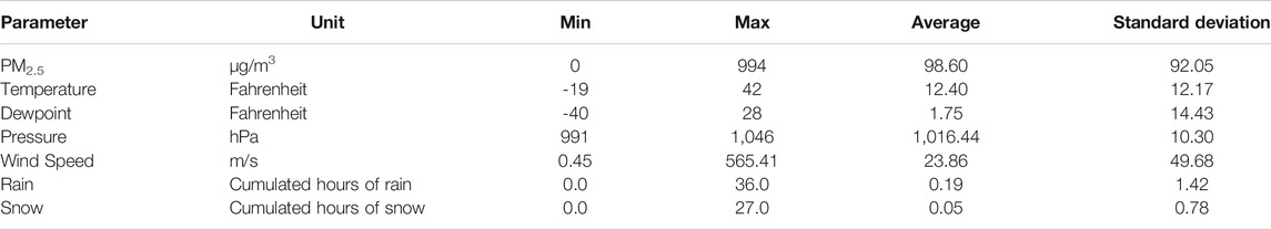
TABLE 1. Parameter description.
Figure 1 shows the heatmap detailing Pearson’s correlation coefficient values between different parameters in data. A gradient from dark blue to white represents positive to negative correlations between different parameters. As can be observed in Figure 1, some of the parameters showed strong correlation values between the dependent and independent variables. For example, dewpoint and temperature showed a strong positive correlation while dewpoint and pressure showed a strong negative correlation. Similary, PM2.5 concentration showed a negative correlation with the wind speed parameter.
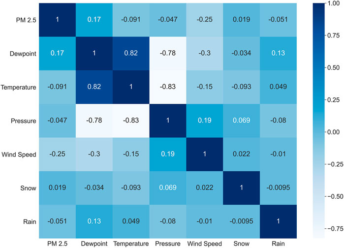
FIGURE 1. Heatmap of the Pearson’s correlation coefficient values for different parameters in data. A gradient from dark blue to white color represents strong positive to strong negative correlations, respectively.
The time-series data were first pre-processed and then converted into a supervised dataset. Missing entries were dropped from the dataset. As the features had different scales, machine learning models could have assigned higher weightage to features with high magnitudes. This differential weighting would have impacted the performance of models. Thus, to resolve the issue, all parameters were normalized using a min-max scaler, and their values were converted into the range [-1, 1]. This range was selected after experimenting with other ranges. A supervised machine learning model requires data in the form of the following equation:
Here, the model takes some input vector x and maps it to some output y. In this paper, we developed models that could forecast PM2.5 6 hours ahead in time, where each prediction was 1-h apart. The following equation represents the input vector that was provided to models:
Here, t represents the specific time period ‘t’ in the data series, and
Here, the input to the model was a normalized series of parameter vectors described in Eq. 2 from some hour
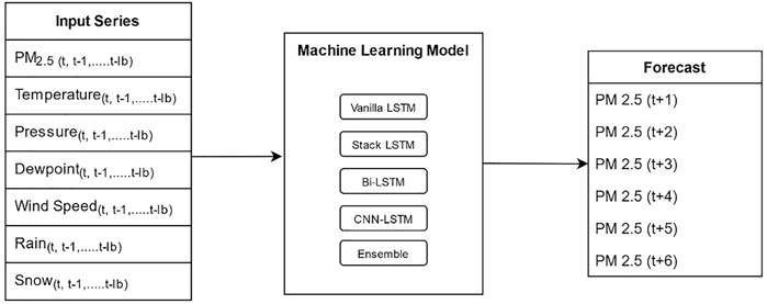
FIGURE 2. High-level model inputs and outputs.
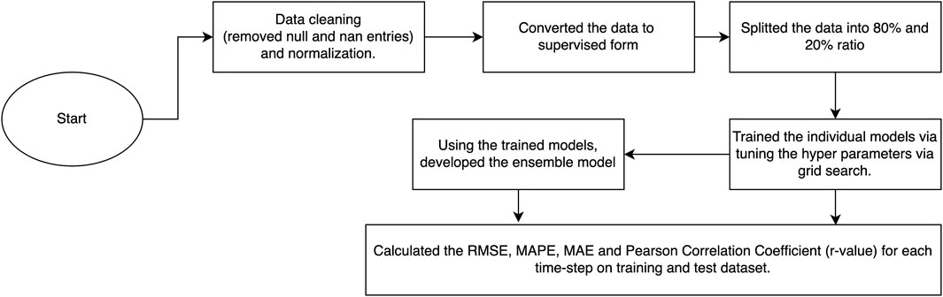
FIGURE 3. Flow-chart of the procedure followed in training models.
For this research, four variants of LSTM models, namely, vanilla-LSTM, stack-LSTM bidirectional-LSTM, and CNN-LSTM, were developed. A weighted average ensemble model using the above-mentioned optimized models was also developed to obtain a regularized model.
Vanilla-LSTM: A vanilla-LSTM model is a variant of the LSTM model with only a single hidden layer. So, it consists of one input layer, one hidden layer of one or multiple LSTM nodes, and an output layer (Kumar et al., 2021). Figure 4 shows the LSTM node with three gates: input gate, forget gate, and output gate. These gates allow the LSTM unit to regulate which information to keep in memory and which to forget. Vanilla-LSTM can have multiples LSTM nodes in its hidden layer.
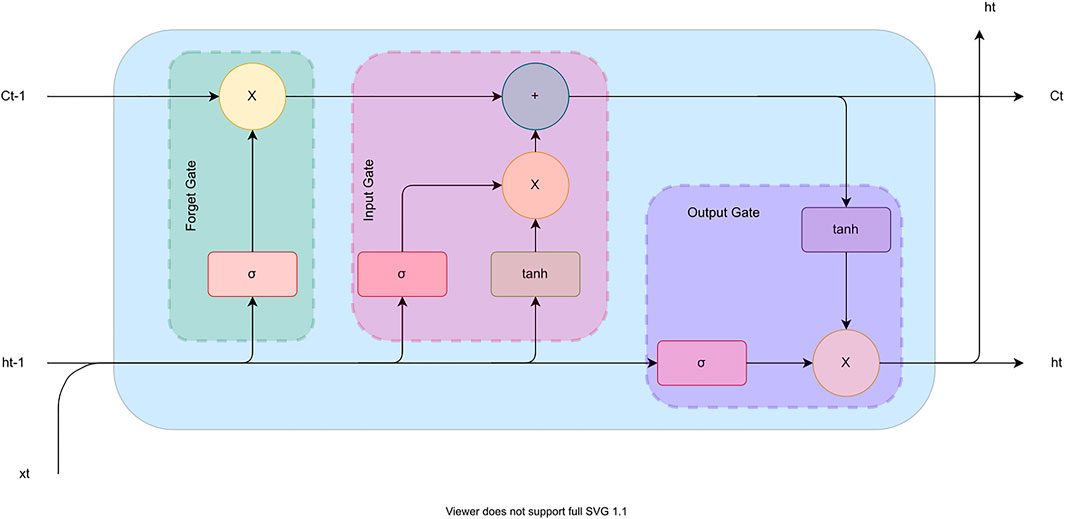
FIGURE 4. The building block of LSTM.
Stack-LSTM: A stack-LSTM model consists of multiple hidden layers (Kumar et al., 2021). So, it has one input layer, a number of hidden layers consisting of a varying number of nodes per layer, and an output layer (Kumar et al., 2021). The LSTM unit depicted in Figure 4 is the same for the stack-LSTM model too.
Bidirectional-LSTM: In the bidirectional-LSTMs model, instead of one, two LSTM units are trained on the same input sequence (Kumar et al., 2021). The first unit of LSTM is trained on the input sequence as it is, and a second LSTM unit is trained on the reversed copy of the input sequence. This technique enables the LSTM to learn additional context or dependency in the data. In this experiment, we developed a stacked bidirectional-LSTM model with a varied number of nodes and layers. Figure 5 shows the architecture of the bidirectional-LSTM model.
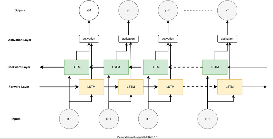
FIGURE 5. The architecture of Bidirectional-LSTM.
CNN-LSTM: In this architecture, a hybrid combination of CNN and LSTM is utilized, where the CNN layer finds the local-spatial relationship, and the LSTM layer finds the temporal relationship in the data (Ding et al., 2018). One 1D-CNN layer followed by 1D max-pooling layer, cascaded with one LSTM layer, is used in the model. The 1D-CNN layer interpreted the input subsequence using the specified filter size and kernel size. The output from the 1D-CNN layer is then passed to a 1D max-pooling layer that distilled the output to its half the size, which includes the most salient features of the data. Then, this distilled data is passed to the LSTM unit for further processing. We optimized the filter size and kernel size in the CNN layer and the number of nodes in the LSTM layer.
Ensemble Model: The weighted average technique is utilized to develop the ensemble model using all the five aforementioned models. Each model contributes to calculating the forecast in the proportion of its performance on the test dataset. The model weights are small positive values and sum up to one. Its numerical value represents the importance in the calculation of forecasting. Eq. 4 shows how the final forecast is calculated in the ensemble model.
Here, Wx is the weight assigned to the model x, and Mx is the forecasted value of the model x. In this research, we first trained and calibrated the above-mentioned individual models. Then, using these calibrated models, we computed the weights for each model in the ensemble model via the grid-search technique.
For training the machine learning model, a root-mean-squared error was used as the loss function, and the Adam optimizer (Kingma & Ba, 2015) was used to optimize the weights of the models. The experiments were executed on a GPU-enabled high-performance cluster, and the experiments were coded using the Keras framework (Ketkar, 2017). The parameters were optimized using the grid-search method. Table 2 shows different model parameters and their ranges. These ranges were choosen based on prior literature concerning these data (Saini et al., 2020). As can be observed from Table 2, for the vanilla-LSTM model, only the number of nodes in its single layer was varied in the set {32, 64, 128, 256}. For the stack-LSTM model, the number of layers and number of nodes per layer was varied in the set {2, 4, 8, 16, 32} and {32, 64, 128, 256}, respectively. For the bidirectional-LSTM model, number of nodes and number of layers were varied in the set {16, 32, 64, 128, 256}, and {1, 2, 4, 8, 16}, respectively. For the CNN-LSTM, filter size, kernel size of CNN, and the number of nodes in the LSTM layer were varied in the set {16, 32, 64}, {1, 3, 5}, and {16, 32, 64, 128}, respectively. Lastly, using the calibrated individual models, the weights for the ensemble model were calculated. Here, the weights were varied in the range of [0, 1], with a step size of 0.01. Other than these parameters, one parameter, i.e., lookback period, was also calibrated for each model and was varied in the set {2, 4, 6, 12}.
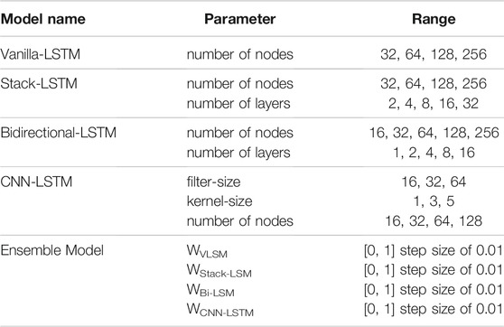
TABLE 2. Parameters of the machine learning model and their ranges.
For the individual models, i.e., vanilla-LSTM, stack-LSTM, bidirectional-LSTM, and CNN-LSTM, the input to the models was the multivariate data from hour ‘t’ to hour ‘t-lb’ (where lb was the lookback period), and the output was the forecasted PM2.5 concentration at hour t+1, t+2, t+3, t+4, t+5, and t+6, respectively. During the training of the models, an error gradient was computed, and it was used to determine the new weights of the neural network. We computed the root mean squared error (RMSE) between actual and predicted values for each hour in the output. Based on the computed RMSE, the weights of the models were updated via the backpropagation method (Leung & Haykin, 1991). For example, if there were 80 observations in the training dataset, 20 observations in the test dataset, and the lookback period was 5, then the observations from one to 5 (actual) were inputted into a model to forecast PM2.5 concentration at hours 6 to 11 (predicted). In the next iteration, observations from two to 6 (actual) were inputted into the model to forecast PM2.5 concentration at hours 7 to 12 (predicted), and so on. The last training would involve inputting observations 69 to 74 (actual) to forecast PM2.5 concentration at hours 75 to 80 (predicted). Similarly, in the test dataset, datapoint 81 to 85 (actual) were inputted into the model to forecast PM2.5 concentration at hours 86 to 91 (predicted), and so on. The last test would involve inputting observations 89 to 94 (actual) to forecast PM2.5 concentration at hours 95 to 100 (predicted). After computing the forecasts in the above-mentioned way, we computed the RMSE between the actual and predicted values for each hour individually and then took its average. This average RMSE was minimized during the training of the models. The difference between training and test was that the parameters of the model were varied during training to minimize the average RMSE across the predicted observations. However, during the test, the best value of parameters found during training was set in the model to predict test values.
For the training of the ensemble model, we utilized the grid-search method to find the optimized weights for each model. Here, the input to the ensemble model was the predicted values of each individual model at hour t+1, t+2, t+3, t+4, t+5, and t+6, and the output was the weighted forecast at hour t+1, t+2, t+3, t+4, t+5, and t+6. Here, t+1, t+2, t+3, t+4, t+5, and t+6 were the PM2.5 future forecasts 1-h, 2-h, 3-h, 4-h, 5-h, and 6-h ahead in time. As the lookback period was different for each model, the starting of the data series was also different. So, to match the data series, we trimmed the initial observations from the dataset (up to the maximum lookback period). For example, if the lookback period for vanilla-LSTM was 6, for stack-LSTM was 4, for bidirectional-LSTM was 8, and for CNN-LSTM was 12, then we trimmed the first 12 observations from the training and test dataset, and the remaining data were used in the training and testing of the ensemble model. So, if there were 80 observations in the training dataset and 20 observations in the test dataset, then after trimming, there were 68 observations in the training dataset and eight observations in the test dataset. The difference between the training and test was that the weights of the ensemble model were varied during the training to minimize the average RMSE across the predicted observations, i.e., we computed the RMSE between the actual and predicted value for each hour and then took its average. This average RMSE was minimized during the training of the ensemble model. However, during the test, the best value of the weights of the ensemble model found during the training was set in the model to predict the test values.
The models were evaluated using four error functions: RMSE, MAPE, MAE and Pearson’s correlation coefficient (r) value. For every model, we calculated the RMSE, MAPE, MAE and r-value separately for each hour. Also, in the training of the models, the average of the RMSEs between the actual and predicted values for each hour was minimized. For example, in vanilla-LSTM, after each epoch, the model computed the RMSE between the actual and predicted values for each hour, i.e., from (t+1) to (t+6), and then took its average. This average RMSE was minimized by the model. Similarly, we trained the other individual models, namely, stack-LSTM, bidirectional-LSTM, and CNN-LSTM. The RMSE penalizes large errors in the forecast. It can be calculated by the following equation:
Where
MAPE is scale-independent, easy to interpret (Kim & Kim, 2016), and it can be calculated by the following equation:
where Actuali represents the ground truth of PM2.5 concentration for the ith data point, Predictedi represents the forecasted value from the model for the ith data point, and
MAE is a measure of errors between paired observations expressing the same phenomenon. MAE is a more natural measure of average error, and it is unambiguous (Willmott & Matsuura, 2005). It can be calculated by the following equation:
Similar to RMSE calculation, in MAPE and MAE error calculations,
Pearson’s correlation coefficient (r) is a measure of linear correlation between two sets of data. The range of r-value is between −1 and 1, where positive values represent positive linear relationships and negative values represent inverse linear relationships between the two sets of data. It can be calculated between actual observations and predicted observations from a model the following equation:
We computed the r value between actual and predicted values for each timestep on both training and test dataset separately. As RMSE, MAPE, MAE, and r are good measures to evaluate the correctness of models, these error functions were used to evaluate and benchmark the developed models.
Table 3 shows the optimized hyperparameter values for each model obtained from the grid search. For the vanilla-LSTM, the lookback period was 6, and the number of nodes was 128. For the stack-LSTM, the lookback period was 4, number of nodes was 128, and the number of layers was 2. For the bidirectional-LSTM, the lookback period was 4, number of nodes was 64, and the number of layers was 2. For the CNN-LSTM, the lookback period was 12, filter-size was 32, kernel-size was 1, and the number of nodes was 32. Lastly, for the ensemble model, the weight parameters for the vanilla-LSTM, stack-LSTM, bidirectional-LSTM, and CNN-LSTM models were 0.13, 0.23, 0.57, and 0.07, respectively. Overall, the bidirectional-LSTM model contributed the most to the ensemble model and its contribution was followed by the stack-LSTM model. The vanilla-LSTM and CNN-LSTM models had fairly smaller contributions to the ensemble model.
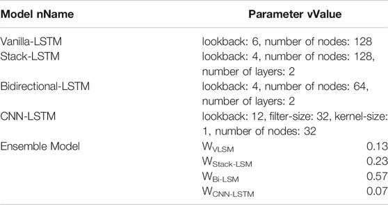
TABLE 3. Calibrated parameter values obtained from the grid-search method in training dataset.
Table 4 shows the hourly RMSE, MAPE, MAE, and the r values for different model predictions ahead in time. For the future hourly forecasts from the vanilla-LSTM model, the RMSE values on the training and test datasets were: 7.95 and 8.04 (hour 1); 22.58 and 21.67 (hour 2); 33.22 and 32.22 (hour 3); 41.34 and 41.7 (hour 4); 47.88 and 49.78 (hour 5); and, 53.29 and 55.6 (hour 6). Similarly, the MAPE for the vanilla-LSTM model on the training and test datasets were: 18.09 and 11.02 (hour 1); 32.88 and 27.03 (hour 2); 48.86 and 41.39 (hour 3); 60.31and 58.13 (hour 4); 70.87and 74.48 (hour 5); and, 89.01 and 87.34 (hour 6). Furthermore, the MAE for the vanilla-LSTM model on the training and test datasets were: 3.43 and 7.53 (hour 1); 12.49 and 14.09 (hour 2); 18.46 and 21.56 (hour 3); 23.88 and 24.88 (hour 4); 28.18 and 31.98 (hour 5); and, 31.66 and 36.20 (hour 6). Finally, the r value for the vanilla-LSTM model on the training and test datasets were: 0.99 and 0.99 (hour 1); 0.97 and 0.91 (hour 2); 0.94 and 0.88 (hour 3); 0.91 and 0.85 (hour 4); 0.87 and 0.80 (hour 5); and, 0.84 and 0.82 (hour 6).
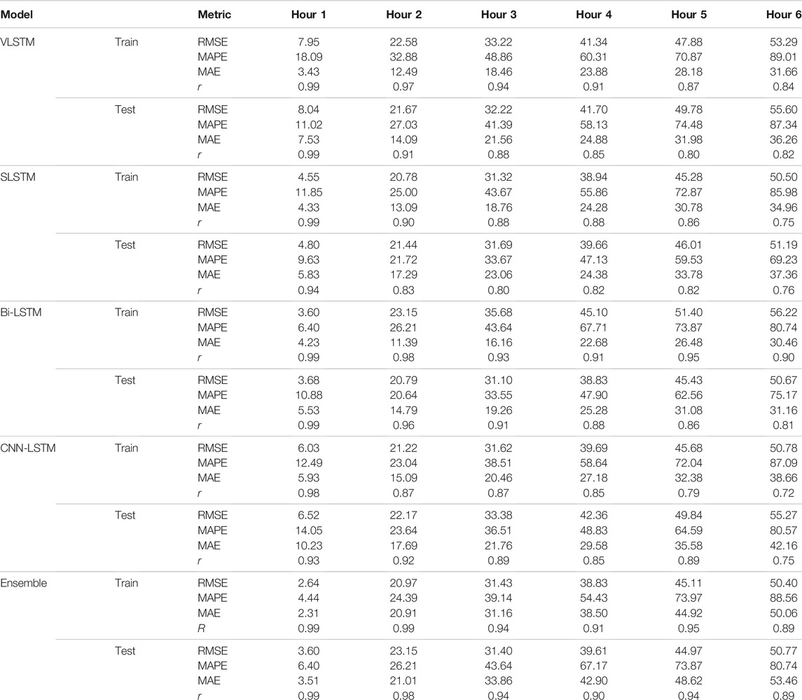
TABLE 4. RMSE (in μg/m3), MAPE (in %), MAE (in μg/m3) and r-value for each individual and ensemble models.
For the future hourly forecasts from the stack-LSTM model, the RMSE values on the training and test datasets were: 4.55 and 4.8 (hour 1); 20.78 and 21.44 (hour 2); 31.32 and 31.69 (hour 3); 38.94 and 39.66 (hour 4); 45.28 and 46.01 (hour 5); and, 50.5 and 51.19 (hour 6). Similarly, the MAPE for the stack-LSTM model on the training and test datasets were: 11.85 and 9.63 (hour 1); 25 and 21.72 (hour 2); 43.67 and 33.67 (hour 3); 55.86 and 47.13 (hour 4); 72.87 and 59.53 (hour 5); and, 85.98 and 69.23 (hour 6). Furthermore, the MAE for the stack-LSTM model on the training and test datasets were: 4.33 and 5.83 (hour 1); 13.09 and 17.29 (hour 2); 18.76 and 23.06 (hour 3); 24.28 and 24.38 (hour 4); 30.78 and 33.78 (hour 5); and, 34.96 and 37.36 (hour 6). Finally, the r value for the stack-LSTM model on the training and test datasets were: 0.99 and 0.94 (hour 1); 0.90 and 0.83 (hour 2); 0.88 and 0.80 (hour 3); 0.88 and 0.82 (hour 4); 0.86 and 0.82 (hour 5); and, 0.75 and 0.76 (hour 6).
For the future hourly forecasts from the bidirectional-LSTM model, the RMSE values on the training and test datasets were: 3.6 and 3.68 (hour 1); 23.15 and 20.79 (hour 2); 35.68 and 31.1 (hour 3); 45.1 and 38.83 (hour 4); 51.4 and 45.43 (hour 5); and, 56.22 and 50.67 (hour 6). Similarly, the MAPE for the bidirectional-LSTM model on the training and test datasets were: 6.4 and 10.88 (hour 1); 26.21 and 20.64 (hour 2); 43.64 and 33.55 (hour 3); 67.71 and 47.9 (hour 4); 73.87 and 62.56 (hour 5); and, 80.74 and 75.17 (hour 6). Furthermore, the MAE for the bidirectional-LSTM model on the training and test datasets were: 4.23 and 5.53 (hour 1); 11.39 and 14.79 (hour 2); 16.16 and 19.26 (hour 3); 22.68 and 25.28 (hour 4); 26.48 and 31.08 (hour 5); and, 30.46 and 31.16 (hour 6). Finally, the r value for the bidirectional-LSTM model on the training and test datasets were: 0.99 and 0.99 (hour 1); 0.98 and 0.96 (hour 2); 0.93 and 0.91 (hour 3); 0.91 and 0.88 (hour 4); 0.95 and 0.86 (hour 5); and, 0.90 and 0.81 (hour 6).
For the future hourly forecasts from the CNN-LSTM model, the RMSE values on the training and test datasets were: 6.02 and 6.52 (hour 1); 21.22 and 22.17 (hour 2); 31.62 and 33.38 (hour 3); 39.69 and 42.36 (hour 4); 45.68 and 49.84 (hour 5); and, 50.78 and 55.27 (hour 6). Similarly, the MAPE for the CNN-LSTM model on the training and test datasets were: 12.49 and 14.05 (hour 1); 23.04 and 23.64 (hour 2); 38.51 and 36.51 (hour 3); 58.64 and 48.83 (hour 4); 72.04 and 64.59 (hour 5); and, 87.09 and 80.57 (hour 6). Furthermore, the MAE for the CNN-LSTM model on the training and test datasets were: 5.93 and 10.23 (hour 1); 15.09 and 17.69 (hour 2); 20.46 and 21.76 (hour 3); 27.18 and 29.58 (hour 4); 32.38 and 35.58 (hour 5); and, 38.66 and 42.16 (hour 6). Finally, the r value for the CNN-LSTM model on the training and test datasets were: 0.93 and 0.98 (hour 1); 0.87 and 0.92 (hour 2); 0.87 and 0.89 (hour 3); 0.85 and 0.85 (hour 4); 0.79 and 0.89 (hour 5); and, 0.72 and 0.75 (hour 6).
For the future hourly forecasts from the ensemble model, the RMSE values on the training and test datasets were: 2.64 and 3.6 (hour 1); 20.97 and 23.15 (hour 2); 31.43 and 31.4 (hour 3); 38.83 and 39.61 (hour 4); 45.11 and 44.97 (hour 5); and, 50.4 and 50.77 (hour 6). Similarly, the MAPE for the ensemble model on the training and test datasets were: 4.44 and 6.4 (hour 1); 24.39 and 26.21 (hour 2); 39.14 and 43.64 (hour 3); 54.43 and 67.17 (hour 4); 73.97 and 73.87 (hour 5); and, 88.56 and 80.74 (hour 6). Furthermore, the MAE for the ensemble model on the training and test datasets were: 2.31 and 3.51 (hour 1); 20.91 and 21.01 (hour 2); 31.16 and 33.86 (hour 3); 38.50 and 42.90 (hour 4); 44.92 and 48.62 (hour 5); and, 50.06 and 53.46 (hour 6). Finally, the r value for the ensemble model on the training and test datasets were: 0.99 and 0.99 (hour 1); 0.99 and 0.98 (hour 2); 0.94 and 0.94 (hour 3); 0.91 and 0.90 (hour 4); 0.95 and 0.94 (hour 5); and, 0.89 and 0.89 (hour 6).
As can be observed from Table 4, for hour 1, the ensemble model had the least RMSE (train: 2.64 μg/m3 and test: 3.6 μg/m3) among all the models. For hour 2, the stack-LSTM had the least RMSE on the training dataset (20.78 μg/m3), while the bidirectional-LSTM had the least RMSE on the test dataset (20.79 μg/m3) among all the models. For hour 3, again, the stack-LSTM had the least RMSE on the training dataset (31.12 μg/m3), while the bidirectional-LSTM had the least RMSE on the test dataset (31.1 μg/m3). For hour 4, the ensemble model had the least RMSE on the training dataset (38.83 μg/m3), while the bidirectional-LSTM had the least RMSE on the test dataset (38.83 μg/m3). For hour 5, the ensemble model had the least RMSE on both train and test dataset (train: 45.11 μg/m3 and test: 44.97 μg/m3). And, finally, for hour 6, the ensemble model had the least RMSE on the training dataset (50.4 μg/m3), while the bidirectional-LSTM had the least RMSE on the test dataset (50.67 μg/m3).
Similarly, for hour 1, the ensemble model had the least MAPE value (train: 4.44% and test: 6.4%). For hour 2, the CNN-LSTM had the least MAPE value on the training dataset (23.04%), while the bidirectional-LSTM had the least MAPE value on the test dataset (20.64%). For hour 3, again, the CNN-LSTM had the least MAPE value on the training dataset (38.51%), while the bidirectional-LSTM had the least MAPE value on the test dataset (33.55%). For hour 4, the ensemble model had the least MAPE value on the training dataset (54.43%), while the bidirectional-LSTM had the least MAPE value on the test dataset (47.13%). For hour 5, the vanilla-LSTM model had the least MAPE value on the training dataset (70.87%), while the stack-LSTM had the least MAPE value on the test dataset (59.53%). And finally, for hour 6, the bidirectional-LSTM model had the least MAPE on the training dataset (80.74%), while the stack-LSTM had the least MAPE value on the test dataset (69.23%).
The overall results in Table 4 show that the errors (RMSE, MAPE, and MAE) increased and the correlation coeffient values decreased as the models predicted from hour one to hour six ahead in time. For certain hours, the test statistics were slightly better compared to the training statistics, which could be due to the different complexities present in training data and test data. It could also be due to the models’ fitting process, where the average RMSE across all 6 h was minimized while training different models.
Figures 6A–F shows the hourly PM2.5 concentration (in µg/m3) forecasts obtained by the ensemble model for the first, second, third, fourth, fifth, and sixth hours ahead in time compared to those observed actually. The x-axis represents the hours from the starting time of the time-series, while the y-axis represents the hourly PM2.5 concentration for a particular hour. For example, in the graph for hour 3, an hourly PM2.5 value at the 12th hour (x-axis) meant that it was the PM2.5 concentration prediction for the 15th hour and it was made at the 12th hour from the starting time (midnight of 01-Jan-2010). Similary, in the graph for hour 2, an hourly PM2.5 value at the 130th hour (x-axis) meant that it was the PM2.5 concentration prediction for the 132 nd h and it was made at the 130th hour from the starting time (midnight of 01-Jan-2010). Plotting all 43,000 observations would have made the graph cluttered and incomprehensible. Thus, only 800 observations from the dataset were plotted. As mentioned in the model calibration section, while training the ensemble model, we trimmed some initial points from the data series (up to the maximum value of lookback period, which was 12). Thus, because of this trimming, the hours start from 12 on the x axis. The first 600 observations in the figure are from the training data, while the remaining 200 are the first 200 observations from the test dataset. In Figure 6, the dotted line separates the train and test data. As can be observed from Figure 6, the actual and predicted values almost overlap each other for different hours. The ensemble model even captured the peaks and troughs present in data.
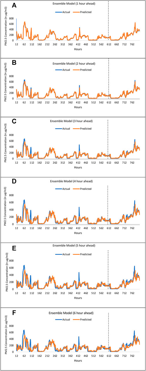
FIGURE 6. Time-series plots of actual and predicted PM2.5 concentrations obtained by the ensemble model for (A) 1 h ahead (B) 2 h ahead (C) 3 h ahead (D) 4 h ahead (E) 5 h ahead, and (F) 6 h ahead.
Models developed and calibrated in this research outperformed the ones developed in the literature (Huang & Kuo, 2018; Jin et al., 2020; Li et al., 2020; Saini et al., 2020). Huang and Kuo (2018) developed APNet for PM2.5 forecasting. The model forecasted one step ahead in time and had the RMSE of 24.228 μg/m3, MAE of 14.63 μg/m3 and the r-value of 0.95. Li et al. (2020) developed a hybrid of CNN and LSTM model for PM2.5 forecasting. Again the model forecasted single step ahead in time. It had the MAE of 13.96 μg/m3 and RMSE of 17.93 μg/m3. Jin et al. (2020) proposed a combination of EMD, CNN, and GRU for PM2.5 forecasting. The proposed model had the RMSE of 46.26 μg/m3 and MAE of 34.59 μg/m3. Lastly, Saini et al. (2020) proposed an ensemble of MLP, LSTM, CNN, and SARIMA models. The proposed ensemble model had the RMSE of 23.45 μg/m3. As can be observed, models developed in this research (including the ensemble model) outperformed prior models developed in literature by a huge margin.
Health implications and the economic impact of deteriorating air quality are well-known (OCED, 2016; World Health Organization, 2018). So, it is crucial to develop forecasting models that can forecast with high accuracy multiple hours ahead in time. Ferlito et al. (2020), Tsai et al. (2018), and Zhao et al. (2019) proposed MLP, vanilla-LSTM, and LSTM-FC model respectively, to forecast PM2.5. Various ensemble techniques were also explored, like Ganesh et al. (2018) and Qiao et al. (2019) proposed an ensemble of three methods, gradient boosting, neural network, and random forest, and stacked autoencoder LSTM (SAE-LSTM), respectively. However, a comprehensive investigation of recurrent neural network type architectures for air quality forecasting still lacked in the literature. Also, techniques like calibration of hyperparameters using grid-search and generalization of the individual models using weighted ensemble techniques were left unexplored.
The primary goal of this research was to bridge the gaps in the literature by developing short- and long-term, highly accurate forecasting models. For this purpose, we developed calibrated recurrent neural networks, namely, vanilla-LSTM, stack-LSTM, bidirectional-LSTM, and CNN-LSTM. We also developed a weighted average ensemble model of the individual LSTM models to achieve better accuracy. Beijing dataset (Liang et al., 2015) was used to train and validate the models. Our results revealed that the developed and calibrated models were able to predict short-term pollution concentration with high accuracy. Experiments also revealed that as the forecasted hour increased, so did the RMSE and MAPE value. These findings are consistent with prior literature (Huang & Kuo, 2018; Feng et al., 2020), where it has been shown that the accuracy degrades as the hour increases. One likely reason can be due to the small size of the dataset; long-term forecasting models generally require a larger dataset. However, the models developed and calibrated in this research outperformed the ones developed in the literature (Huang & Kuo, 2018; Feng et al., 2020; Jin et al., 2020; Li et al., 2020; Saini et al., 2020). Higher accuracy of the developed models can be attributed to the techniques employed in this research, i.e., the systematic calibration of hyperparameters of the models via the grid-search technique, which was absent in the literature.
Results from the experiments also revealed that the weighted average ensemble model performed the best among all the models. The RMSE and MAPE value were the lowest for the ensemble model. A likely reason for this finding could be that the ensemble model was able to generalize the output by taking the best out of the forecasts of the individual models. This generalization leads to higher accuracy. Among the individual models, bidirectional-LSTM outperformed the other models, i.e., vanilla-LSTM, stack-LSTM, and CNN-LSTM. A likely reason for this result can be attributed to the capability of bidirectional-LSTM to process input in the forward as well as in the backward direction, first, on the input sequence as-is and then on a reversed copy of the input sequence. This increases the amount of information available to the network, improving the context available to the network. Again, these findings are consistent with prior literature where Bidirectional-LSTM had performed better than its counterparts (Zhang et al., 2021). However, the Zhang et al. (2021) study only investigated the bidirectional-LSTM model, and other recurrent neural network models were not investigated. In our experimentation, we investigated a wide variety of RNN models by calibrating the models using the grid-search technique.
It was also found that there were certain hours where the loss metrics on the training data were a little higher compared to the loss metrics computed on test data. One likely reason for this finding could be that, for such hours, the complexity of the training data was likely much more than that in test data. It could also be due to model fitting process where the average RMSE across all 6 h was minimized. Overall, models developed in this research (including the ensemble model) outperformed prior models developed in literature by a huge margin.
This research has several implications in the real world. The forecast results from the ensemble models could be used to devise long-term governmental policies. The short- and long-term forecast will help policymakers to take immediate steps to curb air pollution. Widespread use of the developed models by local environmental authorities will complement their day-to-day work. Based on the results from the model, they can make informed, dynamic decisions. Also, a fusion of the developed models with the real-time air-quality monitoring stations will create an ecosystem where using live data, the model can forecast pollutant concentration in real-time. This ecosystem will also help the public to remain vigilant about the deteriorating air quality in their surroundings. The developed models can also be used to generate a timely warning to the public.
Future research may build upon this work where one includes other pollutant parameters, like, ozone, nitrogen oxides, sulphur oxides, and carbon oxides, for the training of the models. One may also experiment with different split-ratios between the test and train data and observe how different splits affect the accuracy of models. We may also include unstructured data, like governmental policies, industrialization, and public perception, to study its effect on the changing air quality. Another aspect to consider is to utilize datasets from other sources (like new established air-quality monitoring stations) to train and validate the developed models. We can also investigate new state-of-the-art machine learning models like time-series generative adversarial network (TGAN) (Goodfellow et al., 2020) and transformers (Vaswani et al., 2017). Some of these ideas form the immediate next steps in our program.
Publicly available datasets were analyzed in this study. This data can be found here: https://archive.ics.uci.edu/ml/datasets/Beijing+PM2.5+Data.
TS contributed to the implementation of the experiment, data analyses, and the development of the models. VD and PC developed the idea of the study, contributed to the design, and writing of the manuscript. All authors contributed to the article and approved the submitted version.
This research work was made possible by a grant from the Department of Environment Science and Technology, Government of Himachal Pradesh, on the project IITM/DST-HP/VD/240 to VD and PC.
The authors declare that the research was conducted in the absence of any commercial or financial relationships that could be construed as a potential conflict of interest.
All claims expressed in this article are solely those of the authors and do not necessarily represent those of their affiliated organizations, or those of the publisher, the editors and the reviewers. Any product that may be evaluated in this article, or claim that may be made by its manufacturer, is not guaranteed or endorsed by the publisher.
We are also grateful for the computational support provided by the Indian Institute of Technology Mandi, HP, India.
Bernard, S., and Kazmin, A. (2018). Dirty Air: How India Became the Most Polluted Country on Earth. London, UK: Financial Times. December 11. Available at: https://ig.ft.com/india-pollution/.
Ding, L., Fang, W., Luo, H., Love, P. E. D., Zhong, B., and Ouyang, X. (2018). A Deep Hybrid Learning Model to Detect Unsafe Behavior: Integrating Convolution Neural Networks and Long Short-Term Memory. Automation in Construction 86, 118–124. doi:10.1016/j.autcon.2017.11.002
Edwards, P. N. (1996). Global Comprehensive Models in Politics and Policymaking. Climatic Change 32 (2), 149–161. doi:10.1007/BF00143706
Feng, R., Gao, H., Luo, K., and Fan, J.-r. (2020). Analysis and Accurate Prediction of Ambient PM2.5 in China Using Multi-Layer Perceptron. Atmos. Environ. 232, 117534. doi:10.1016/j.atmosenv.2020.117534
Ferlito, S., Bosso, F., De Vito, S., Esposito, E., and Di Francia, G. (2020). LSTM Networks for Particulate Matter Concentration Forecasting. Lecture Notes Electr. Eng. 629, 409–415. doi:10.1007/978-3-030-37558-4_61
Ganesh, S. S., Arulmozhivarman, P., and Tatavarti, V. S. N. R. (2018). Prediction of PM2.5 Using an Ensemble of Artificial Neural Networks and Regression Models. J. Ambient Intell. Hum. Comput 0, 1–11. doi:10.1007/s12652-018-0801-8
Goodfellow, I., Pouget-Abadie, J., Mirza, M., Xu, B., Warde-Farley, D., Ozair, S., et al. (2020). Generative Adversarial Networks. Commun. ACM 63 (11), 139–144. doi:10.1145/3422622
Huang, C.-J., and Kuo, P.-H. (2018). A Deep Cnn-Lstm Model for Particulate Matter (Pm2.5) Forecasting in Smart Cities. Sensors 18 (7), 2220. doi:10.3390/s18072220
Irfan, U. (2018). India’s Pollution Levels Are Some of the Highest in the World. Here’s why. - Vox. Vox, October 31. Available at: https://www.vox.com/2018/5/8/17316978/india-pollution-levels-air-delhi-health
Jin, X.-B., Yang, Nian-Xiang., Yang, N.-X., Wang, X.-Y., Bai, Y.-T., Su, T.-L., et al. (2020). Deep Hybrid Model Based on EMD with Classification by Frequency Characteristics for Long-Term Air Quality Prediction. Mathematics 8 (2), 214. doi:10.3390/math8020214
Ketkar, N. (2017). “Introduction to Keras,” in Deep Learning with Python, Apress, 97–111. doi:10.1007/978-1-4842-2766-4_7
Kim, S., and Kim, H. (2016). A New Metric of Absolute Percentage Error for Intermittent Demand Forecasts. Int. J. Forecast. 32 (3), 669–679. doi:10.1016/j.ijforecast.2015.12.003
Kingma, D. P., and Ba, J. L. (2015). “Adam: A Method for Stochastic Optimization,” in 3rd International Conference on Learning Representations, ICLR 2015 - Conference Track Proceedings. 22, https://arxiv.org/abs/1412.6980v9.
Kumar, P., Sihag, P., Sharma, A., Pathania, A., Singh, R., Chaturvedi, P., et al. (2021). Prediction of Real-World Slope Movements via Recurrent and Non-recurrent Neural Network Algorithms: A Case Study of the Tangni Landslide. Indian Geotech J. 51, 788–810. 23. doi:10.1007/s40098-021-00529-4
Leung, H., and Haykin, S. (1991). The Complex Backpropagation Algorithm. IEEE Trans. Signal. Process. 39 (9), 2101–2104. doi:10.1109/78.134446
Li, T., Hua, M., and Wu, X. (2020). A Hybrid CNN-LSTM Model for Forecasting Particulate Matter (PM2. 5). Ieeexplore.Ieee.Org. Available at: https://ieeexplore.ieee.org/abstract/document/8979420/. doi:10.1109/access.2020.2971348Accessed April 26, 2021)
Liang, X., Zou, T., Guo, B., Li, S., Zhang, H., Zhang, S., et al. (2015). Assessing Beijing's PM 2.5 Pollution: Severity, Weather Impact, APEC and winter Heating. Proc. R. Soc. A. 471, 20150257. 2182. doi:10.1098/rspa.2015.0257
OCED (2016). The Economic Consequences of Outdoor Air Pollution (Paris, France: OECD). doi:10.1787/9789264257474-en
Pozza, S. A., Lima, E. P., Comin, T. T., Gimenes, M. L., and Coury, J. R. (2010). Time Series Analysis of PM2.5 and PM10−2.5 Mass Concentration in the City of Sao Carlos, Brazil. Ijep 41 (1–2), 90–108. doi:10.1504/IJEP.2010.032247
Qiao, W., Tian, W., Tian, Y., Yang, Q., and Access, Y. W.-I. (2019). Undefined. (n.dThe Forecasting of PM2. 5 Using a Hybrid Model Based on Wavelet Transform and an Improved Deep Learning Algorithm. Ieeexplore.Ieee.Org. Available at: https://ieeexplore.ieee.org/abstract/document/8853331/(Accessed April 26, 2021).
Saini, T., Tomar, G., Rana, D. C., Attri, S., and Dutt, V. (2020). “December)A Weighted Ensemble Approach to Real-Time Prediction of Suspended Particulate Matter,” in International Advanced Computing Conference, Singapore (Springer), 381–394.
Tsai, Y., Zeng, Y., and on, Y. C. (2018). Air Pollution Forecasting Using RNN with LSTM. Ieeexplore.Ieee.Org. I. 16th I. C., & 2018, undefined. (n.d.). Available at: https://ieeexplore.ieee.org/abstract/document/8512020/(Accessed April 26, 2021).
Vaswani, A., Shazeer, N., Parmar, N., Uszkoreit, J., Jones, L., Gomez, A. N., et al. (2017). Attention Is All You Need. Advances in Neural Information Processing Systems, 5999–6009. Available at: https://arxiv.org/abs/1706.03762v5 (Accessed 2017. December)
Wieland, V., and Wolters, M. H. (2012). Forecasting and Policy Making. IMFS Working Paper Series. Available at: https://ideas.repec.org/p/zbw/imfswp/62.html
Willmott, C., and Matsuura, K. (2005). Advantages of the Mean Absolute Error (MAE) over the Root Mean Square Error (RMSE) in Assessing Average Model Performance. Clim. Res. 30 (1), 79–82. doi:10.3354/cr030079
World Health Organization. (2018). Ambient (Outdoor) Air Pollution. https://www.who.int/news-room/fact-sheets/detail/ambient-(outdoor)-air-quality-and-health.
Zhang, Z., Zeng, Y., and Yan, K. (2021). A Hybrid Deep Learning Technology for PM2.5 Air Quality Forecasting. Environ. Sci. Pollut. Res., 1–14. doi:10.1007/s11356-021-12657-8
Keywords: PM25, forecasting, vanilla-LSTM, stack-LSTM, bidirectional-LSTM, CNN-LSTM, ensemble
Citation: Saini T, Chaturvedi P and Dutt V (2021) Modelling Particulate Matter Using Multivariate and Multistep Recurrent Neural Networks. Front. Environ. Sci. 9:752318. doi: 10.3389/fenvs.2021.752318
Received: 02 August 2021; Accepted: 22 November 2021;
Published: 09 December 2021.
Edited by:
Hilkka Timonen, Finnish Meteorological Institute, FinlandReviewed by:
Martha Arbayani Zaidan, University of Helsinki, FinlandCopyright © 2021 Saini, Chaturvedi and Dutt. This is an open-access article distributed under the terms of the Creative Commons Attribution License (CC BY). The use, distribution or reproduction in other forums is permitted, provided the original author(s) and the copyright owner(s) are credited and that the original publication in this journal is cited, in accordance with accepted academic practice. No use, distribution or reproduction is permitted which does not comply with these terms.
*Correspondence: Varun Dutt, varun@iitmandi.ac.in
Disclaimer: All claims expressed in this article are solely those of the authors and do not necessarily represent those of their affiliated organizations, or those of the publisher, the editors and the reviewers. Any product that may be evaluated in this article or claim that may be made by its manufacturer is not guaranteed or endorsed by the publisher.
Research integrity at Frontiers
Learn more about the work of our research integrity team to safeguard the quality of each article we publish.