 Yizhuo Wen1
 Aili Yang
- 1Key Laboratory for Environmental Biotechnology of Higher Education of Fujian Province, Xiamen University of Technology, Xiamen, China
- 2College of Fundamental Science, Beijing Polytechnic, Beijing, China
A Bayesian-model-averaging Copula (i.e., BMAC) approach was proposed for correlation analysis of monthly rainfall and runoff in Xiangxi River watershed, China. The BMAC approach was formulated by incorporating existing Bayesian model averaging (i.e., BMA) method and Archimedean Copula techniques (e.g., Gumbel-Hougaard, Clayton and Frank Copulas) within a general bivariate hydrologic correlation analysis framework. In this paper, the BMA method was applied to determine the marginal distribution functions of variables, and the Copula method was used to analyze the correlation. Results showed that: 1) the BMA method could improve the representation of the marginal distribution of hydrological variables with smaller corresponding errors; 2) the predictive joint distributions of monthly rainfall and runoff was much better calibrated by the Gumbel Copula according to criteria of the root mean square error (i.e., RMSE), Akaike Information Criterion (i.e., AIC) values, Anderson-Darling test (i.e., AD test), and Cramer-von Mises test (i.e., CM test); and 3) the bivariate joint probability and return periods of rainfall and runoff based on the optimal Copula function was characterized and the monthly rainfall and runoff presented a strong positive correlation based on Kendall and Spearman’s rank correlation coefficients. Therefore, the BMAC approach performed reasonably well and can be further used to simulate runoff values according to the historical and predicted rainfall data. Highlights: 1) A Bayesian-model-averaging Copula method is proposed for correlation analysis; 2) the monthly rainfall and runoff in Xiangxi River watershed has a positive correlation. 3) Gumbel Copula is the best in modelling the joint distributions in the Xiangxi River watershed.
1 Introduction
Investigating the hydrological variables relations is of vital significance for flood control and water resource management (Fan et al., 2018). Univariate hydrological frequency analysis procedures are important tools for analyzing the change rules between rainfall and runoff (Andres-Domenech et al., 2015; Shin et al., 2015; Zhou et al., 2020). However, it cannot reflect the variation of variables effectively because it overlooks the joint effects of variables. In addition, variables of real-world hydrological systems are complicated with many factors, such as correlations and multidimensional characteristics in hydrological processes (Zhang et al., 2006; Zhang et al., 2007; Remesan et al., 2009; Reusser et al., 2010; Takbiri and Ebtehaj, 2017; Sun and Zhou, 2020). Consequently, statistical theories of joint probability analysis were undertaken for developing more effective methods in this field.
As a sufficient probabilistic analysis method for correlated multivariate events, Copula function has been widely applied to hydrological simulations (Aghakouchak et al., 2010; Chebana et al., 2012; Ma et al., 2013; Serinaldi, 2013; Madadgar and Moradkhani, 2014; Qiang et al., 2014; Li and Zheng, 2016; Nasr and Chebana, 2019.; Yang et al., 2019). One of the advantages is that the calculations of marginal distributions and correlation analysis in Copula function are relatively independent, which is the successful key to make the joint analysis of multivariate methods more popular (Favre et al., 2004; Shiau et al., 2007; Chebana and Ouarda, 2009; Sraj et al., 2015; Sugimoto et al., 2016; Lei et al., 2018). On the other hand, the inherent uncertainty has been proved by practices existing in any single frequency distribution model structure (See and Abrahart, 2001; Wu et al., 2022), which directly affects the reliability of hydrological prediction (Zhou et al., 2018). Therefore, a multi-model method is proposed to deal with the inherent uncertainty for improving the accuracy of hydrological modeling and forecasting. Currently, the multi-model combination methods include: the weighted average method, linear regression, and neural networks (DeChant and Moradkhani, 2014; Xu et al., 2017; Zhou et al., 2021). These methods are mainly based on different deterministic theories to form a more accurate synthesis simulation results, but rarely consider the uncertainty of the model structure. Therefore, a better method to reflect the uncertainty of the multi-model method is particularly important.
The Bayesian model averaging (BMA) method has been widely used to construct a simulation process with better description of variables’ probabilities in areas of management, medicine, meteorology, etc. (Tsai, 2010; Fang et al., 2018; Zhang and Yang, 2018). It can efficiently handle the marginal probability distribution function (Zhang and Yang, 2012) and produce more accurate model synthesis results for the uncertain model structure. In this case, the obtained marginal distribution functions can be directly used as inputs of the Copula function. However, the adjunct process has not been used to study the correlation between rainfall and runoff, and thus its applicability remains to be further verified.
When considering the structure of the marginal distribution in the present hydrological field, a single model is usually used to calculate the hydrological frequency curve of each variable (Xu et al., 2021). General models of distribution of unique hydrological probabilities include primarily Gamma distribution, generalized extreme value distribution, lognormal distribution, etc. (Lu et al., 2021). According to the principle of the BMA method, it is found that we can construct a more suitable expression form for specific hydrological variables through this method and use this distribution form as a marginal distribution to calculate the Copula joint distribution function (Lin et al., 2021; Rahimi et al., 2021). Compare with the non-parametric method. Non-parametric methods are generally robust but ineffective. The precision of the parameter estimates is high. Ramsey proposed a method for modelling the core and imported histograms into the model. This method not only improves the accuracy of the estimate, but also increases the design speed (Ramsey, 2012). The nonparametric method gives more attention to sample distribution as it does not take the form of distribution. However, when the quantity of data is different, the parameter method is more stable because of the a priori assumption that it responds to a specific distribution. When the amount of data is small, using the parameter method and considering its underestimated risk can obtain better results (Zeng, 2014). Therefore, in this paper, we compare the marginal distribution among the parameter, nonparametric, and BMA methods to choose the best method of this study.
The objective of this article is to develop a BMA Copula (BMAC) approach for correlation analysis with rainfall-runoff in the Xiangxi River, the largest tributary of the Yangtze River in the Hubei part of the Three Gorges Reservoir area. In this system, the marginal distributions of monthly rainfall and runoff are simulated by the BMA method with better description in probability of each variable. Then correlation analysis between rainfall and runoff is constructed by the Gumbel Copula method. This paper aims to: 1) determine the variables’ marginal distribution functions; 2) estimate the two-dimensional Copula function parameters and calculate the Kendall and Spearman’s rank correlation coefficients to ascertain the optimal Copula function; and 3) characterize the bivariate joint probability and return periods of rainfall and runoff based on the optimal Copula function.
2 Methodology
2.1 Bayesian Model Averaging Theory
2.1.1 Bayesian Model Averaging
BMA is a statistical analysis method and can be used to infer a probabilistic prediction. It is a statistical analytical method that considers the uncertainty of the model itself. In this paper, the BMA method is applied to simulate the streamflow. Suppose that y is the forecasted variable,
where
Let
where
2.1.2 Expectation Maximization Algorithm
To effectively calculate the weight and variance of BMA, the expectation-maximization (EM) method is introduced in this paper. EM is an iterative calculation method and has been widely used (Bilmes, 1998) to calculate the maximum likelihood estimation, and the obtained results show good effect especially in dealing with a great number of missing data. In detail, the EM algorithm can be illustrated as follows.
Considering the stability and convenience of calculation, the EM algorithm uses log-likelihood function (Duan et al., 2006). Assume the prediction error in time and space is independent, the log-likelihood function can be formulated as follows (Duan et al., 2006):
Assume
Step 1. Initialization:
where
Step 2. Calculate the initial likelihood:
Step 3. Implementation of the E-step operation:
Step 4. Perform the M-step operation:Calculate the weights of the single prediction model:
Update the single forecast model variance:
Update the value of the likelihood function
Step 5. Check convergence:If
2.1.3 Kernel Density Estimation
In statistics, the kernel density estimation (KDE) is a non-parametric way to estimate the probability density function of a random variable. KDE is a fundamental data smoothing problem where inferences about the population are made, based on a finite data sample (Li et al., 2022). Among the many non-parametric methods currently used, the KDE method proposed by Guo et al. (1996) is the most widely used, and the effect is the most ideal.
The estimation formula of the univariate kernel probability density function:
where
2.2 Copula Function Theory
Copula theory was proposed by Sklar (1959), which has many types of Copula functions, such as normality of Copula, t-Copula functions, and Archimedean Copula function family (Nelsen, 1999). Among them, Archimedean Copula function family, including Gumbel-Hougaard Copula function, Clayton Copula function, and Frank Copula functions, has characteristics of simplified structure, diversification, and practicability, which lead to relatively simple processes in constructing corrections among variables (Xie et al., 2020). Consequently, the Archimedean Copula function family could be an important method for hydrologic frequency analysis.
2.2.1. Archimedean Copula Function
Let ui be the variable margin,
(1) Gumbel-Hougaard Copula function
(2) Clayton Copula function
(3) Frank Copula function
2.2.2 Correlation Measure of Copula
Correlation measure of random variables is used to describe the mutual dependence between random variables. There are many test metrics, in this study Kendall’s rank correlation coefficient
2.2.3 Estimation of Copula Function Parameter
To estimate the parameter of Copula function, the exact maximum likelihood (EML) method is used (Dupuis, 2007). If the joint distribution function of t-dimensional continuous random variables
Step 1. Establish the relevant likelihood functionThe joint density function is expressed as:
Likelihood function is expressed as:
Correspondingly, the log-likelihood function can be expressed as:
Step 2. Solve the likelihood function
where:
2.3 Goodness-Of-Fit Statistical Tests
In order to perform the goodness-of-fit statistic tests for both univariate distribution and Copula functions the root mean square error (RMSE) and Akaike Information Criterion (AIC) are adopted to assess the validation of the BMAC method. RMSE can quantitatively analyze the results when the graph fitting effect is similar. To evaluate the performance and select the best fitted Copulas, the goodness-of-fit statistics test is conducted based on AIC (Akaike, 1974) and Cramér von Mises statistics (Genest et al., 2009).
where
The Kolmogorov-Smirnov test (K-S test) is chosen because it is a useful nonparametric hypothesis test, which is primarily used to test if a set of samples comes from some probability distribution (Miller, 1956).
where
The Anderson-Darling test (AD test) also has been chosen because of its excellent properties against a variety of alternatives, the test statistic is as follows (D'Agostino, 1986):
where:
Specific calculation steps are as follows:
Step 1. Calculate the marginal distribution functions
Step 2. Calculate
where:
Step 3. Calculate statistic value
Step 4. Estimate Copula parameter
Step 5. Simulate and generate Copula random samples with Rosenblatt’s transformation test method, find new Copula function parameter
Step 6. Calculate a new
Step 7. Repeat steps 3 to 6
Step 8. Compare the relationship between the statistic
2.4 Bayesian-Model-Averaging Copula (BMAC) Method
In this study, the BMAC method would be proposed by combining the BMA and Copula methods into a general framework. In detail, the BMA method is used to determine the marginal distributions of monthly rainfall and runoff, and the Archimedean Copula method can be used to construct the joint distribution of monthly rainfall of runoff. Correspondingly, the BMAC method involves four steps: 1) determining the marginal distributions of monthly rainfall and runoff based on the principle of BMA and generating the values of weight through the EM method, 2) establishing the joint distributions by the Archimedean Copula (e.g., Gumbel-Hougaard Copula, Clayton Copula, and Frank Copula) method, 3) estimating the values of the Copula parameter
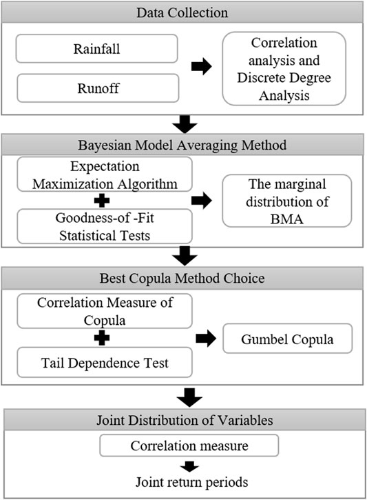
FIGURE 1. The framework of BMAC.
3 Case Study
3.1 Overview of the Studied Area
The Xiangxi River basin is located between 30.96 ∼ 31.67° N and 110.47 ∼ 111.13°E in the Hubei part of China, being the largest tributary of the Yangtze River in the Three Gorges Reservoir area (see Figure 2). It originates in the Shennongjia Nature Reserve, with the mainstream length of 94 km and a catchment area of 3,099 km2 (Han et al., 2014). This region experiences a northern subtropics climate, and the main rainfall season is from May to September with the annual precipitation of 1,100 mm (Xu et al., 2009). In addition, the hydrological station mostly covering this river is called the Xiangshan Hydrological Station (110.45°E, 31.13°N).
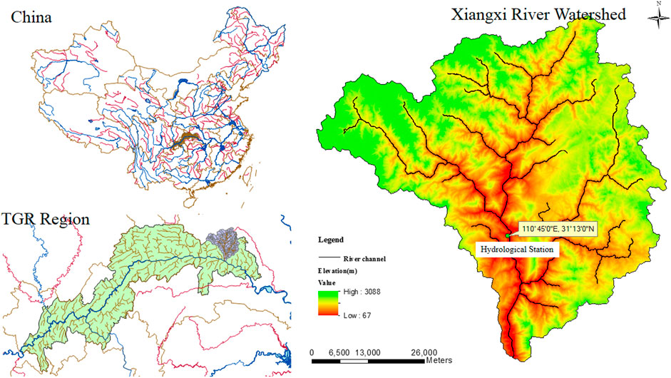
FIGURE 2. The Studied are (Fan et al., 2016).
In order to provide decision support for flood control and water resource management of the Xiangxi River basin, the hydrological frequency analysis of this region would be studied based on daily rainfall and runoff data (1991–2008) from Xingshan Hydrological Station in this study (see Figure 3). Figure 3 demonstrates that rainfall and runoff in 1996 were relatively high, while rainfall and runoff in 1997 were relatively low. The annual distribution of runoff is primarily concentrated. The annual distribution of rainfall is rather dispersed. Annual rainfall and runoff during 1996 and 2007 were particularly sparse. Rainfall and runoff are strongly correlated. Figure 4 demonstrates that the distribution of monthly rainfall and runoff are similar. The scatter plot demonstrates that the R-square value is 0.698 and the AUK value of the Kendall plot is 0.667. Both of them show a positive correlation (Figure 5).
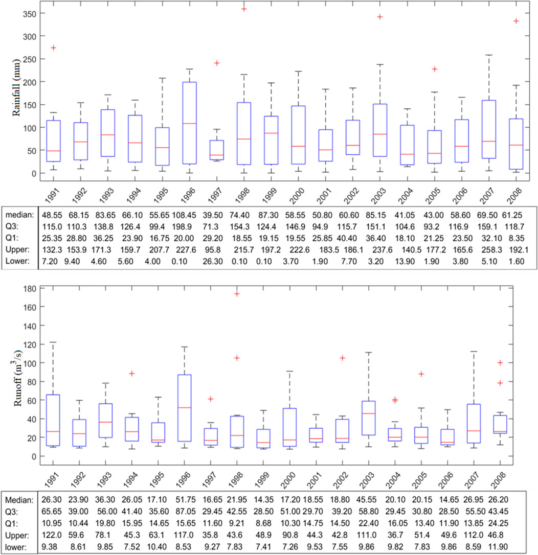
FIGURE 3. The boxspots of monthly rainfall and runoff in the Xiangxi River watershed. Median id the midlevel line of the data, Upper and Lower are the maximum and minimum values, Q1 and Q3 are the lower and upper quantities.
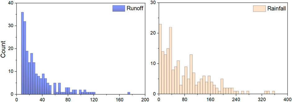
FIGURE 4. The Histogram of mothly rainfall and runoff in the Xiangxi River watershed.
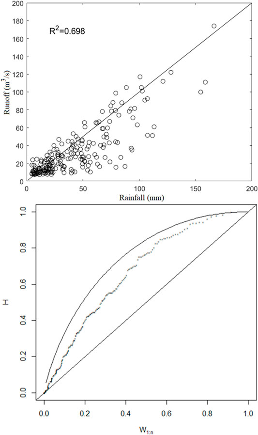
FIGURE 5. The Scatter plot and Kendall plot of monthly rainfall and runoff. The top one is Scatter plot and the bottom one is Kendall plot.
3.2 Results Analysis
3.2.1 Comparison of Marginal Distributions
In the procedure of hydrological frequency analysis, the monthly rainfall and runoff probability distributions in the Xiangxi River basin are first estimated by the Gamma, the generalized extreme value, and the lognormal distributions, respectively. And then, the BMA-based marginal distributions are obtained according to the three estimated distributions. Table 1 shows the fitting parameters of probability distributions.
TABLE 1. The fitting parameters of probability distributions.
Based on the weights and distribution parameters presented above, the BMA-based marginal distributions of monthly rainfall and runoff can be obtained. The Gamma distribution may account for a major proportion (99.99%) to produce the BMA-based marginal distribution of monthly rainfall; while the generalized extreme value distribution and lognormal distribution may account for almost the same proportion to produce the BMA-based marginal distribution of monthly runoff.
The comparison of empirical and generated marginal cumulative distribution functions (CDFs) for monthly rainfall and runoff is shown in Figure 6. It indicates that the BMA-based marginal distribution may appropriately represent the univariate rainfall and runoff probability distributions. In order to clearly clarify, the D, RMSE, and AIC values for the marginal distributions obtained by the four methods are also calculated and presented in Table 2. In addition, to compare with the non-parametric methods, the KDE method is also calculated in the same way. Results D show that only the GEV and BMA methods pass the K-S test (the upper boundary of D is 0.092 while alpha is 0.05) in both rainfall and runoff. The obtained results indicate the corresponding errors of the BMA method are relatively smaller suggesting the accuracy of the marginal distributions generated by the BMA method is very excellent.
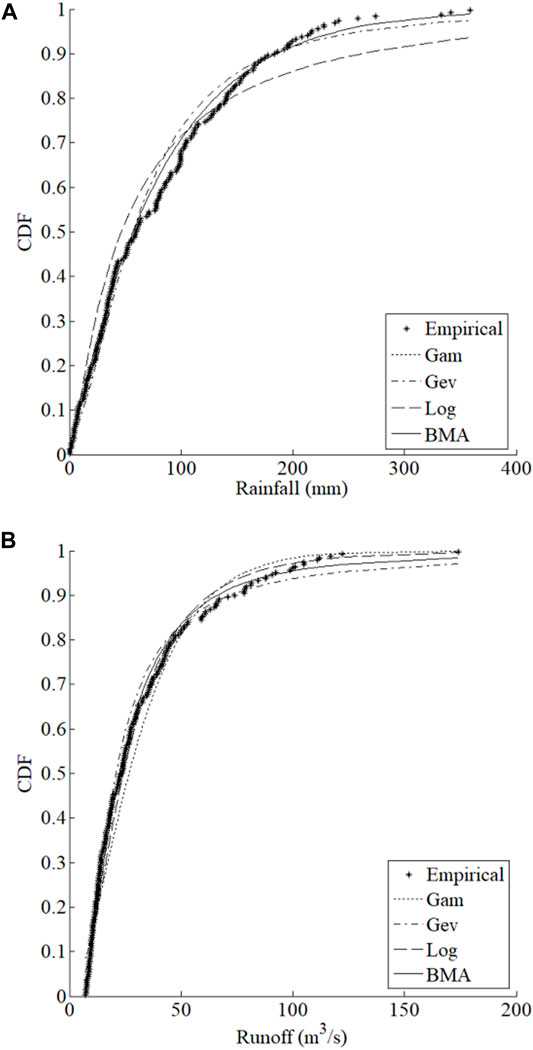
FIGURE 6. Comparison of the generated and empirical marginal CDFs for mothly rainfall (A) and runoff (B).
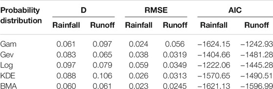
TABLE 2. The D, RMSE and AIC analysis for marginal distributions.
3.2.2 Comparison of Joint Distributions
After determining marginal distributions, the joint probability distributions of monthly rainfall and runoff in the Xiangxi River can be estimated by a Copula function. The estimation parameters for each Copula function are calculated based on the maximum likelihood estimation theory. In addition, according to the obtained parameters, the correlation coefficients can be calculated. Results are given in Table 3. It can be seen that the Kendall’s rank correlation coefficient ranges from 0.42 to 0.59 and the Spearman’s rank correlation coefficient ranges from 0.56 to 0.78. Therefore, it can be concluded that the monthly rainfall and runoff of the Xiangxi River have a relatively strong positive correlation.
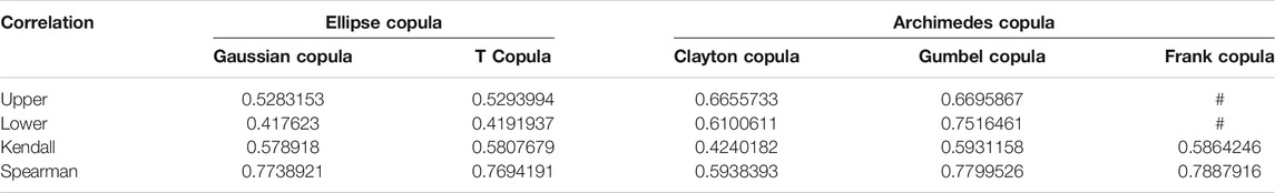
TABLE 3. Parameters estimation and correlation analysis of copula function.
According to Table 3, Gumbel-Hougaard-Copula-based joint distribution and Frank-Copula-based joint distribution are superior to the Clayton one based on the Kendall correlation and the Spearman correlation. Moreover, it shows that the estimation of the upper tail correlation coefficient should select the Gumbel Copula, the number is 0.6696. The estimation of the lower tail correlation coefficient should select the Gumbel Copula, the number is 0.7516. Obviously, there are both upper tail correlation and lower tail correlation in the Xiangxi River. This conforms to research by Yang et al. (2016). Goodness-of-fit tests of empirical joint CDFs and theoretical joint CDFs are calculated for further analysis (as shown in Figure 7).
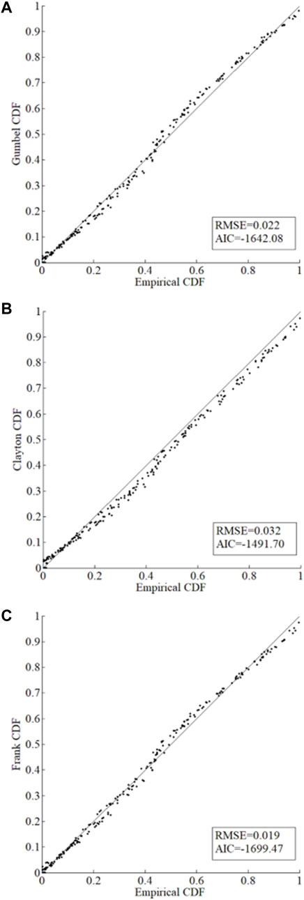
FIGURE 7. Comparison of the theotrical and empircal joint CDFs for rainfall and runoff in Xiangxi River. (A) Gumbell-Hougard-Copula-based joint distribution. (B) Frank-Copula-based joint distribution, respectively.
Comparing the results shown in Figure 7, it can be known that the joint distribution by Frank-Copula is close to the one by Gumbel-Hougaard-Copula in quantifying the relevant characteristics of monthly rainfall and runoff of the Xiangxi River. The RMSE of the Gumbel-Hougaard-Copula is less than the Clayton copula. The Frank-Copula function has no tail correlation and cannot capture the tail correlation between variables according to Xue (2018). Gumbel Copula performs better in the upper correlation while Clayton Copula performs better in the lower correlation (Jondeau, 2016). Therefore, the Gumbel Copula function would be chosen to construct the joint distribution of monthly rainfall-runoff pairs. The corresponding results are plotted and shown in Figure 8. Figure 9 shows the combined probability density and return period of rainfall and runoff using the Gumbel Copula. It indicates that the extreme value of annual precipitation or annual runoff, the joint probability density is relatively small. When the annual runoff is constant, the greater the annual precipitation, the longer the time of return period is. In addition, the largest rainfall of observed data is 1,341.7 mm, the runoff of that year is 556.36 m3/s. The return period is about 10 years, which is reasonable.
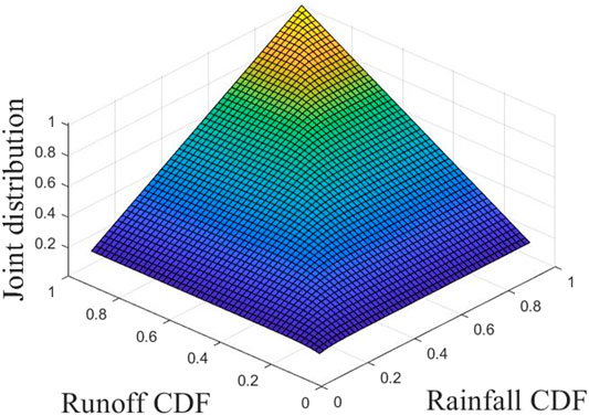
FIGURE 8. The joint CDFs of rainfall and runoff.
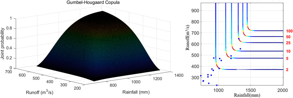
FIGURE 9. Joint probability density and return periods of rainfall and runoff.
In this study, the AD test and the CM test also have been selected to investigate the suitability of the BMAC-based joint distributions in describing the dependencies for different rainfall-runoff pairs. The results are displayed in Table 4, and statistics
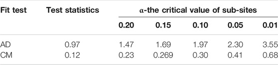
TABLE 4. Goodness-of-fit of BMAC.
3.2.3 Comparison of BMAC and MEGHC
In order to further clarify the efficiency of the BMAC method, a Maximum Entropy-Gumbel-Hougaard Copula (MEGHC) method proposed by Kong et al. (2015) has been applied for comparison. Accordingly, two joint distributions can be generated by the two methods, and the bias value between the two methods also can be obtained (shown in Figure 10). From Figure 10, the results are quite close to each other, and the great deviation value (i.e., absolute error) is 0.03, which illustrates that both of the two methods can be used to generate the joint distribution of the rainfall and runoff because of the best fitting effect. It also can be found that, under the condition of the CDF interval being 0–0.4, results obtained by the BMAC method are superior to the MEGHC method; while the CDF interval being 0.9–1, the MEGHC method may converge much faster. To some extent, the MEGHC method can better capture the characteristics of the upper tail dependence, which plays a great role in flood and drainage control and watershed design work (Kong et al., 2015). However, in the situation of representing the uncertainty of the model structure, it is hard to find a suitable distribution to capture the characteristic of the hydrologic variable. Comparatively, the BMAC method can obtain a synthetic simulation result especially in exactly reflecting the variables’ correlations.
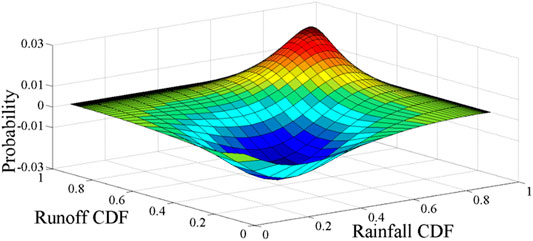
FIGURE 10. Comparison of BMAC and MEGHC.
4 Conclusion
In this study, a BMAC method has been proposed for assessing correlations of bivariate variables in hydrological processes. Through incorporating BMA and Copula functions within a general framework, BMAC can determine the marginal distribution functions of variables, and meanwhile analyze the correlation. To demonstrate the applicability, the developed BMAC method also has been adopted to investigate the hydrological frequency analysis of the Xiangxi River basin. The specific conclusions can be summarized as follows:
(1) Compared with the empirical and nonparametric marginal CDFs, the Bayesian model averaging method can improve the representation of the marginal distribution of hydrological variables and comprehensively capture the shape of empirical CDF with smaller corresponding errors.
(2) The goodness-of-fit statistical tests, consisting of RMSE, K-S, and AD test, indicate that the BMAC method is suitable for describing the statistical probabilities and the dependencies in the historical data of the Xiangxi River, China.
(3) There is a relatively strong positive correlation existing between the monthly rainfall and runoff. The Gumbel Copula would be best for modelling the joint distributions of monthly rainfall and runoff.
(4) Compared with the MEGHC method proposed by Kong et al. (2015), the BMAC method can obtain more accurate synthesis results when the model structure is evaluated as uncertain.
(5) The accuracy of the BMAC method in modelling the joint distribution of hydrological variables would be influenced by the performance of the marginal distribution of the variables and the algorithm used for estimating the unknown parameters in Copula functions. Consequently, further studies are required to analyze the uncertainty of the calculation process.
Data Availability Statement
The raw data supporting the conclusion of this article will be made available by the authors, without undue reservation.
Author Contributions
YW conceived and designed the method of BMAC, collected the data and analyzed the results, and wrote the manuscript. AY conceived and designed the method. XK collected the data and analyzed the results. YS analyzed the results. All authors read and approved the final manuscript.
Funding
This research was funded by the Natural Science Foundation of Fujian Province, China (2021J011180).
Conflict of Interest
The authors declare that the research was conducted in the absence of any commercial or financial relationships that could be construed as a potential conflict of interest.
Publisher’s Note
All claims expressed in this article are solely those of the authors and do not necessarily represent those of their affiliated organizations, or those of the publisher, the editors, and the reviewers. Any product that may be evaluated in this article, or claim that may be made by its manufacturer, is not guaranteed or endorsed by the publisher.
Acknowledgments
The authors thank the support from the Hydrologic Bureau of Xingshan County.
References
Aghakouchak, A., Bárdossy, A., and Habib, E. (2010). Conditional Simulation of Remotely Sensed Rainfall Data Using a Non-gaussian V-Transformed Copula. Adv. Water Resour. 33, 624–634. doi:10.1016/j.advwatres.2010.02.010
Akaike, H. (1974). A New Look at the Statistical Model Identification. IEEE Trans. Automat. Contr. 19, 716–723. doi:10.1109/tac.1974.1100705
Andrés-Doménech, I., García-Bartual, R., Montanari, A., and Marco, J. B. (2015). Climate and Hydrological Variability: the Catchment Filtering Role. Hydrol. Earth Syst. Sci. 19, 379–387. doi:10.5194/hess-19-379-2015
Bilmes, J. A. (1998). A Gentle Tutorial of the EM Algorithm and its Application to Parameter Estimation for Gaussian Mixture and Hidden Markov Models. Berkeley: Department of Electrical Engineering and Computer Science U. C, 1–13.
Chebana, F., Dabo-Niang, S., and Ouarda, T. B. M. J. (20122012). Exploratory Functional Flood Frequency Analysis and Outlier Detection. Water Resour. Res. 48. doi:10.1029/2011WR011040John Wiley & Sons
Chebana, F., and Ouarda, T. B. M. J. (2009). Index Flood-Based Multivariate Regional Frequency Analysis. Water Resour. Res. 45, W10435. doi:10.1029/2008WR007490
D'Agostino, R. (1986). Goodness-of-Fit-Techniques. Cleveland, OH, USA: CRC Press. ISBN 978-135-144-455-2.
Dai, Q., Han, D., Rico-Ramirez, M., and Srivastava, P. K. (2014). Multivariate Distributed Ensemble Generator: A New Scheme for Ensemble Radar Precipitation Estimation over Temperate Maritime Climate. J. Hydrol. 511, 17–27. doi:10.1016/j.jhydrol.2014.01.016
DeChant, C. M., and Moradkhani, H. (2014). Toward a Reliable Prediction of Seasonal Forecast Uncertainty: Addressing Model and Initial Condition Uncertainty with Ensemble Data Assimilation and Sequential Bayesian Combination. J. Hydrol. 519, 2967–2977. doi:10.1016/j.jhydrol.2014.05.045
Duan, Q., Ajami, N. K., Gao, X., and Sorooshian, S. (2007). Multi-model Ensemble Hydrologic Prediction Using Bayesian Model Averaging. Adv. Water Resour. 30, 1371–1386. doi:10.1016/j.advwatres.2006.11.014
Dupuis, D. J. (2007). Using Copulas in Hydrology: Benefits, Cautions, and Issues. J. Hydrologic Eng. 12, 383–393. doi:10.1061/(ASCE)1084-0699(2007)12:4(381)
Fan, Y., Huang, G., Zhang, Y., and Li, Y. (2018). Uncertainty Quantification for Multivariate Eco-Hydrological Risk in the Xiangxi River within the Three Gorges Reservoir Area in China. Engineering 4, 617–626. doi:10.1016/j.eng.2018.06.006
Fan, Y. R., Huang, W. W., Huang, G. H., Huang, K., Li, Y. P., and Kong, X. M. (2016). Bivariate Hydrologic Risk Analysis Based on a Coupled Entropy-Copula Method for the Xiangxi River in the Three Gorges Reservoir Area, China. Theor. Appl. Climatol 125, 381–397. doi:10.1007/s00704-015-1505-z
Fang, G., Guo, Y., Huang, X., Rutten, M., and Yuan, Y. (2018). Combining Grey Relational Analysis and a Bayesian Model Averaging Method to Derive Monthly Optimal Operating Rules for a Hydropower Reservoir. Water 10, 1099. doi:10.3390/w10081099
Favre, A.-C., El Adlouni, S., Perreault, L., Thiémonge, N., and Bobée, B. (2004). Multivariate Hydrological Frequency Analysis Using Copulas. Water Resour. Res. 40. doi:10.1029/2003WR002456
Genest, C., Rémillard, B., and Beaudoin, D. (2009). Goodness-of-fit Tests for Copulas: A Review and a Power Study. Insurance: Maths. Econ. 44, 199–213. doi:10.1016/j.insmatheco.2007.10.005
Guo, S. L., Kachroo, R. K., and Mngodo, R. J. (1996). Nonparametric Kernel Estimation of Low Flow Quantiles. J. Hydrol. 185, 335–348. doi:10.1016/0022-1694(95)02956-7
Han, J.-C., Huang, G.-H., Zhang, H., Li, Z., and Li, Y.-P. (2014). Bayesian Uncertainty Analysis in Hydrological Modeling Associated with Watershed Subdivision Level: a Case Study of SLURP Model Applied to the Xiangxi River Watershed, China. Stoch Environ. Res. Risk Assess. 28, 973–989. doi:10.1007/s00477-013-0792-0
Jondeau, E. (2016). Asymmetry in Tail Dependence in Equity Portfolios. Comput. Stat. Data Anal. 100, 351–368. doi:10.1016/j.csda.2015.02.014
Kong, X. M., Huang, G. H., Fan, Y. R., and Li, Y. P. (2015). Maximum Entropy-Gumbel-Hougaard Copula Method for Simulation of Monthly Streamflow in Xiangxi River, China. Stoch Environ. Res. Risk Assess. 29, 833–846. doi:10.1007/s00477-014-0978-0
Lei, X.-H., Tan, Q.-F., Wang, X., Wang, H., Wen, X., Wang, C., et al. (2018). Stochastic Optimal Operation of Reservoirs Based on Copula Functions. J. Hydrol. 557, 265–275. doi:10.1016/j.jhydrol.2017.12.038
Li, F., and Zheng, Q. (2016). Probabilistic Modelling of Flood Events Using the Entropy Copula. Adv. Water Resour. 97, 233–240. doi:10.1016/j.advwatres.2016.09.016
Li, G., Wang, Y. X., Zeng, Y., and He, W. X. (2022). A New Maximum Entropy Method for Estimation of Multimodal Probability Density Function. Appl. Math. Model. 102, 137–152. doi:10.1016/j.apm.2021.09.029
Lin, K., Zhou, J., Liang, R., Hu, X., Lan, T., Liu, M., et al. (2021). Identifying Rainfall Threshold of Flash Flood Using Entropy Decision Approach and Hydrological Model Method. Nat. Hazards 108, 1427–1448. doi:10.1007/s11069-021-04739-0
Lu, L., Yuan, W., Su, C., Gao, Q., Yan, D., and Wu, Z. (2021). Study on the Early Warning and Forecasting of Flash Floods in Small Watersheds Based on the Rainfall Pattern of Risk Probability Combination. Stoch Environ. Res. Risk Assess. doi:10.1007/s00477-021-02059-0
Ma, M., Song, S., Ren, L., Jiang, S., and Song, J. (2013). Multivariate Drought Characteristics Using Trivariate Gaussian and Student T Copulas. Hydrol. Process. 27, 1175–1190. doi:10.1002/hyp.8432
Madadgar, S., and Moradkhani, H. (2014). Improved B Ayesian Multimodeling: Integration of Copulas and B Ayesian Model Averaging. Water Resour. Res. 50, 9586–9603. doi:10.1002/2014WR015965
McLachlan, G. J., and Krishnan, T. (1997). The EM Algorithm and Extensions. 2nd ed. Hoboken, NJ, USA: Wiley, 274. ISBN 978-047-120-170-0.
Miller, L. H. (1956). Table of Percentage Points of Kolmogorov Statistics. J. Am. Stat. Assoc. 51, 111–121. doi:10.1080/01621459.1956.10501314
Nasr, I. B., and Chebana, F. (2019). Multivariate L-Moment Based Tests for Copula Selection, with Hydrometeorological Applications. J. Hydrol. 579, 124151. doi:10.1016/j.jhydrol.2019.124151
Nelsen, R. B. (1999). An Introduction to Copulas. New York, NY, USA: Springer. ISBN 978-038-728-678-5.
Raftery, A. E., Balabdaoui, F., Gneiting, T., and Polakowski, M. (2003). “Using Bayesian Model Averaging to Calibrate Forecast Ensembles,”. Technical Report, no. 440 (Seattle, Washington: Department of Statistics, University of Washington). doi:10.21236/ada459828
Rahimi, L., Deidda, C., and Demichele, C. (2021). Origin and Variability of Statistical Dependencies between Peak, Volume, and Duration of Rainfall-Driven Flood Events. Sci. Rep. 11, 1. doi:10.1038/s41598-021-84664-1
Ramsey, C. B. (2012). The Use of Kernel Density Estimates to Assist in the Identification of Volcanic Tephra. Quatern. Int. 2012, 279–280. doi:10.1016/j.quaint.2012.07.309
Remesan, R., Shamim, M. A., Han, D., and Mathew, J. (2009). Runoff Prediction Using an Integrated Hybrid Modelling Scheme. J. Hydrol. 372, 48–60. doi:10.1016/j.jhydrol.2009.03.034
Reusser, D. E., Buytaert, W., and Zehe, E. (2011). Temporal Dynamics of Model Parameter Sensitivity for Computationally Expensive Models with the Fourier Amplitude Sensitivity Test. Water Resour. Res. 47, W07551. doi:10.1029/2010WR009947
See, L., and Abrahart, R. J. (2001). Multi-model Data Fusion for Hydrological Forecasting. Comput. Geosciences 27, 987–994. doi:10.1016/S0098-3004(00)00136-9
Serinaldi, F. (2013). An Uncertain Journey Around the Tails of Multivariate Hydrological Distributions. Water Resour. Res. 49, 6527–6547. doi:10.1002/wrcr.20531
Shiau, J.-T., Feng, S., and Nadarajah, S. (2007). Assessment of Hydrological Droughts for the Yellow River, China, Using Copulas. Hydrol. Process. 21, 2157–2163. doi:10.1002/hyp.6400
Shin, M.-J., Guillaume, J. H. A., Croke, B. F. W., and Jakeman, A. J. (2015). A Review of Foundational Methods for Checking the Structural Identifiability of Models: Results for Rainfall-Runoff. J. Hydrol. 520, 1–16. doi:10.1016/j.jhydrol.2014.11.040
Sklar, A. (1959). Fonctions de répartition à n dimensions et leurs marges, (N-dimensional distribution function and its margin in 1959), Vol. 8. Paris, French: Publications de l'Institut de Statistique de l'Uni- versité de Paris, 229–231.
Sraj, M., Bezak, N., and Brilly, M. (2015). Bivariate Flood Frequency Analysis Using the Copula Function: a Case Study of the Litija Station on the Sava River. Hydrol. Process. 29, 225–238. doi:10.1002/hyp.10145
Sugimoto, T., Bárdossy, A., Pegram, G. G. S., and Cullmann, J. (2016). Investigation of Hydrological Time Series Using Copulas for Detecting Catchment Characteristics and Anthropogenic Impacts. Hydrol. Earth Syst. Sci. 20, 2705–2720. doi:10.5194/hess-20-2705-2016
Sun, C., and Zhou, X. (2020). Characterizing Hydrological Drought and Water Scarcity Changes in the Future: A Case Study in the Jinghe River Basin of China. Water 12, 1605. doi:10.3390/w12061605
Takbiri, Z., Ebtehaj, A. M., and Foufoula-Georgiou, E. (2017). A Multi-Sensor Data-Driven Methodology for All-Sky Passive Microwave Inundation Retrieval. Hydrol. Earth Syst. Sci. 21, 2685–2700. doi:10.5194/hess-21-2685-2017
Tsai, F. T.-C. (2010). Bayesian Model Averaging Assessment on Groundwater Management under Model Structure Uncertainty. Stoch Environ. Res. Risk Assess. 24, 845–861. doi:10.1007/s00477-010-0382-3
Wu, R.-T., Jokar, M., Jahanshahi, M. R., and Semperlotti, F. (2022). A Physics-Constrained Deep Learning Based Approach for Acoustic Inverse Scattering Problems. Mech. Syst. Signal Process. 164, 108190. doi:10.1016/j.ymssp.2021.108190
Xie, W. P., Yang, J. S., Yao, R. J., and Wang, X. P. (2020). Impact Study of Impoundment of the Three Gorges Reservoir on Salt-Water Dy-Namics and Soil Salinity in the Yangtze River Estuary. J. Environ. Inform. 36, 11–23. doi:10.3808/jei.202000432
Xu, B., Huang, X., Mo, R., Zhong, P.-a., Lu, Q., Zhang, H., et al. (2021). Integrated Real-Time Flood Risk Identification, Analysis, and Diagnosis Model Framework for a Multireservoir System Considering Temporally and Spatially Dependent Forecast Uncertainties. J. Hydrol. 600, 126679. doi:10.1016/j.jhydrol.2021.126679
Xu, H., Taylor, R. G., Kingston, D. G., Jiang, T., Thompson, J. R., and Todd, M. C. (2010). Hydrological Modeling of River Xiangxi Using SWAT2005: A Comparison of Model Parameterizations Using Station and Gridded Meteorological Observations. Quat. Int. 226, 54–59. doi:10.1016/j.quaint.2009.11.037
Xu, Y., Huang, G., and Fan, Y. (2017). Multivariate Flood Risk Analysis for Wei River. Stoch Environ. Res. Risk Assess. 31, 225–242. doi:10.1007/s00477-015-1196-0
Xue, Y. (20182018). Coupla-based Tail Correlation Theory and its Application. Yichang, China: Sanxia University, 1–37.
Yang, A. L., Huang, G. H., Kong, X. M., and Hao, Z. D. (2016). Analysis of Rainfall-Runoff Correlation in Xiangxi River Basin Based on Maximum Entropy-Copula Method. South-to-North Water Transfers Water Sci. Technol. 14, 84–89. doi:10.13476/j.cnki.nsbdqk.2016.01.014
Yang, P., Xia, J., Zhang, Y., Zhan, C., and Sun, S. (2019). How Is the Risk of Hydrological Drought in the Tarim River Basin, Northwest China? Sci. Total Environ. 693, 133555. doi:10.1016/j.scitotenv.2019.07.361
Zeng, H. (2014). Comparative Study on the Methods of Determining the Insurance Premium Rates of Crops in the Region. Xinjiang, China: Xinjiang University of Finance and Economics.
Zhang, L., and Singh, V. P. (2006). Bivariate Flood Frequency Analysis Using the Copula Method. J. Hydrol. Eng. 11, 150–164. doi:10.1061/(ASCE)1084-0699(2006)11:2(150)
Zhang, L., and Singh, V. P. (2012). Bivariate Rainfall and Runoff Analysis Using Entropy and Copula Theories. Entropy 14, 1784–1812. doi:10.3390/e14091784
Zhang, L., and Singh, V. P. (2007). Bivariate Rainfall Frequency Distributions Using Archimedean Copulas. J. Hydrol. 332, 93–109. doi:10.1016/j.jhydrol.2006.06.033
Zhang, L., and Yang, X. (2018). Applying a Multi-Model Ensemble Method for Long-Term Runoff Prediction under Climate Change Scenarios for the Yellow River Basin, China. Water 10, 301. doi:10.3390/w10030301
Zhou, X., Huang, G., Li, Y., Lin, Q., Yan, D., and He, X. (2021). Dynamical Downscaling of Temperature Variations over the Canadian Prairie Provinces under Climate Change. Remote Sensing 13, 4350. doi:10.3390/rs13214350
Zhou, X., Huang, G., Wang, X., and Cheng, G. (2018). Future Changes in Precipitation Extremes over Canada: Driving Factors and Inherent Mechanism. J. Geophys. Res. Atmos. 123, 5783–5803. doi:10.1029/2017JD027735
Keywords: archimedean copula, Bayesian model averaging, rainfall and runoff, Xiangxi river watershed, climate change
Citation: Wen Y, Yang A, Kong X and Su Y (2022) A Bayesian-Model-Averaging Copula Method for Bivariate Hydrologic Correlation Analysis. Front. Environ. Sci. 9:744462. doi: 10.3389/fenvs.2021.744462
Received: 20 July 2021; Accepted: 29 November 2021;
Published: 18 January 2022.
Edited by:
Yurui Fan, Brunel University London, United KingdomReviewed by:
Md Shahid Latif, University of Western Ontario, CanadaWei Fang, Xi’an University of Technology, China
Copyright © 2022 Wen, Yang, Kong and Su. This is an open-access article distributed under the terms of the Creative Commons Attribution License (CC BY). The use, distribution or reproduction in other forums is permitted, provided the original author(s) and the copyright owner(s) are credited and that the original publication in this journal is cited, in accordance with accepted academic practice. No use, distribution or reproduction is permitted which does not comply with these terms.
*Correspondence: Aili Yang, eWFuZ2FpbGlsb3lAZ21haWwuY29t