Towards a Living Lab for Enhanced Thermal Comfort and Air Quality: Analyses of Standard Occupancy, Weather Extremes, and COVID-19 Pandemic

Maintaining indoor environmental (IEQ) quality is a key priority in educational buildings. However, most studies rely on outdoor measurements or evaluate limited spatial coverage and time periods that focus on standard occupancy and environmental conditions which makes it hard to establish causality and resilience limits. To address this, a fine-grained, low-cost, multi-parameter IOT sensor network was deployed to fully depict the spatial heterogeneity and temporal variability of environmental quality in an educational building in Sydney. The building was particularly selected as it represents a multi-use university facility that relies on passive ventilation strategies, and therefore suitable for establishing a living lab for integrating innovative IoT sensing technologies. IEQ analyses focused on 15 months of measurements, spanning standard occupancy of the building as well as the Black Summer bushfires in 2019, and the COVID-19 lockdown. The role of room characteristics, room use, season, weather extremes, and occupancy levels were disclosed via statistical analysis including mutual information analysis of linear and non-linear correlations and used to generate site-specific re-design guidelines. Overall, we found that 1) passive ventilation systems based on manual interventions are most likely associated with sub-optimum environmental quality and extreme variability linked to occupancy patterns, 2) normally closed environments tend to get very unhealthy under periods of extreme pollution and intermittent/protracted disuse, 3) the elevation and floor level in addition to room use were found to be significant conditional variables in determining heat and pollutants accumulation, presumably due to the synergy between local sources and vertical transport mechanisms. Most IEQ inefficiencies and health threats could be likely mitigated by implementing automated controls and smart logics to maintain adequate cross ventilation, prioritizing building airtightness improvement, and appropriate filtration techniques. This study supports the need for continuous and capillary monitoring of different occupied spaces in educational buildings to compensate for less perceivable threats, identify the room for improvement, and move towards healthy and future-proof learning environments.

Introduction

It is widely acknowledged that, in developed countries, people spend the majority of their time indoors. In the United States, it is estimated that 87% of the time is allocated to indoor activities (Klepeis et al., 2001), while in Australia, the percentage reaches 90% (Australian Government, 2020). These figures are expected to soar in the next decades as a consequence of the progressive dispossession of outdoor public spaces caused by 1) deterioration of urban liveability, 2) escalation of overheating episodes, and 3) intensification of weather extremes (IPCC Fifth Assessment Report (AR5), 2013; Santamouris, 2020). This poses an urgent need for providing adequate indoor environmental quality (IEQ), specifically in buildings that host vulnerable populations and a high density of users, or those whose occupants require long-lasting preservation of attention, productivity, and health. Educational buildings feature all these criteria and thus represent a priority target for IEQ assessments (Eide et al., 2010; Simons et al., 2010; Mendell et al., 2013).

In educational facilities, such as schools and universities, maximizing students’ and staff’s performance while preventing absenteeism is a basic, yet challenging requirement particularly due to the wide range of possible metabolic rates, clothing levels, and activities that typify the user category (Havenith, 2007; Kim et al., 2009). These variables arbitrate whether a defined indoor air quality and thermal condition can negatively impact the occupants’ cognitive performance by altering the decision-making ability (Satish et al., 2012) or productivity (Wyon, 2004; Ebenstein et al., 2016). Beyond comfort and efficiency, multiple studies on educational facilities indicate that failure to manage indoor air quality could increase the risk of acute and chronic effects on students’ physical and mental health (Loh and Andamon; Annesi-Maesano et al., 2013; Andualem et al., 2019). Indoor air pollution impairs cognitive functions, damages the nervous system, increases ischaemic stroke risk, depression, and mood disorders in adult populations (Calderón-Garcidueñas et al., 2015; Taylor et al., 2015) and even more in infants and youngsters (Gent et al., 2003). Further, extensive evidence demonstrates the negative health impacts of different pollutants indoors, such as ozone (O₃) and fine particles (Mi et al., 2006; Zhao et al., 2015), as well as nitrogen dioxide (NO₂), carbon monoxide (CO), volatile organic compounds (VOCs) and benzene, toluene, ethylbenzene, xylenes (BTEX) (Chen et al., 2000; Evrard et al., 2006). An overview of challenges and impacts can be found in (Chatzidiakou et al., 2012).

Comparatively underexplored are the damaging effects of extreme ambient environmental stressors, such as heatwaves or wildfires. These further exacerbate the range and severity of health deterioration (Saggu et al., 2018; Reid et al., 2019), but the topic-specific literature is sparse. The risk assessment of human exposure to health-threatening indoor environmental conditions, and consequently the choice of containment measures and risk prevention, are critical tasks that need to be adequately informed (Rocca et al., 2020). This further motivates a fine-grained, site-specific monitoring of exposure to environmental stressors (Nazarian and Lee, 2021) as well as smart control of rooms, such that we compensate for less perceivable threats, passive ventilation inefficiencies, and excessive energy consumption.

A variety of studies reveals that occupants are rather insensitive to most Sick Building Syndrome (SBS) drivers. For instance, in Haverinen-Shaughnessy et al. (2015), ventilation rate, temperature, and hygiene of high contact surfaces manifested as health- and performance-threatening IEQ parameters in classrooms. A 70-school district in the United States was monitored during two academic years in terms of ambient air temperature (T), relative humidity (RH) and carbon dioxide (CO₂). Settled dust and cleaning effectiveness, as well as student data (socioeconomic background, absenteeism, performance, and number of visits to school nurse) was recorded. Significant associations were stricken between high academic grades and levels of T and CO₂ as well as between CO₂/culturable bacteria and medical visits due to respiratory or gastrointestinal symptoms. Furthermore, IEQ measurements and perception analyses in nine naturally ventilated schools in Athens, Greece (Dorizas et al., 2015) revealed that PM and CO₂ levels were significantly and positively correlated with SBS symptoms, scholastic performance, and health symptoms. However, the personal perception of IAQ degradation was rather insensitive to increased levels of particulate matter, while being strongly correlated with temperature variations. This is in line with (Stazi et al., 2017), according to which temperature was the key driver for students’ control actions on ventilation, while CO₂ increments went unnoticed.

Other studies highlight that passive buildings, even those built upon sustainability principles, are prone to inadequate ventilation. Almeida and de Freitas (2014) verified the IEQ impacts of the rehabilitation of school buildings via retrofitting in Portugal. They monitored annual T, RH, CO₂, and ventilation rates in 24 classrooms across nine school buildings, out of which seven were retrofitted. Non-retrofitted buildings were compared against retrofitted schools with HVAC or natural/mechanical ventilation systems. Statistical analyses and simulations confirmed that 1) the ventilated schools were the best-performing, 2) non-retrofitted schools provided inadequate IEQ throughout the year, and 3) retrofitted classrooms were affected by the limited use of mechanical ventilation, thus experiencing serious overheating episodes. Further IEQ analyses in a secondary school Germany (Ortiz Perez et al., 2018) demonstrate the complexity of maintaining adequate IEQ levels in passively ventilated classrooms even in case of high frequency of ventilation, pointing towards the need for capillary monitoring and control of rooms, also for energy minimisation. The same inefficiency was found in passively ventilated school buildings in Italy (Schibuola and Tambani, 2020). An experimental campaign was carried out in wintertime in four classrooms having similar shape, size, occupancy pattern, windows type, and dimensions and the interlink between IAQ, ventilation rate, Hazard Index, and Cancer Risk was investigated. It was found that 1) in absence of appreciable internal pollution sources, the indoor concentrations of chemical pollutants were correlated to the corresponding outdoor concentrations and 2) manual operation of ventilation controls was insufficient to guarantee acceptable IAQ levels over 24 h. To tackle such a need for smart ventilation in schools, a sense-and-act approach in a secondary school is proposed in (Stazi et al., 2017) where an automatic system opens and closes the hopper windows based on Humphreys’ adaptive algorithm (Humphreys et al., 2013) with coefficients adjusted to the specific climate and CO₂ levels. The research was carried out in two similar and adjacent classrooms, one equipped with the automatic system, one left to manual operation. Results proved that CO₂ and T comfort levels easily surpassed the acceptable range in both classrooms, however, the automated system promptly restored acceptable levels, while control actions in the manually-operated classroom (particularly associated with CO₂ levels) were typically untimely. A similar approach was proposed in Sydney, Australia (Haddad et al., 2021), where two adjacent classrooms were characterized in terms of infiltration and ventilation rate, and were monitored to measure thermal comfort and air quality during the school year. One room only was equipped with a cloud-connected, demand-controlled mechanical ventilation system. Under automatic control of air extraction, CO₂ levels were largely maintained within comfortable and attention-preserving levels. Peak values were shaved by nearly 70% as compared to the free-running twin classroom.

Previous studies support the need for high spatial and temporal resolution monitoring of IEQ in educational buildings to track its distinctive variability, which can then feed into human-centric and automated control actions for enhanced air quality and thermal comfort. So far, however, limited studies have deployed expansive sensor networks that also provide a long-term assessment of educational buildings for different environmental conditions and occupancy patterns. The emergence of low-cost, internet-enabled environmental sensors aims to address this shortcoming, establishing educational buildings as living labs for integrating innovative sensing, data analytics, and automated control methods that enhance IEQ. An example of such large-scale Internet-of-Things (IoT) sensor deployment in schools is seen in (Palacios Temprano et al., 2020), where 280 classrooms hosting nearly 10,000 children are continuously monitored for 5 years. Preliminary results reveal how indoor climate conditions differ considerably across classrooms and throughout the academic year, indicating that sensors need to be installed in each individual classroom and for at least one academic year to build up accurate, longitudinal IEQ assessments and capture causal links. The heterogeneity of IEQ is further exacerbated in university buildings - where occupants are more diverse (encompassing students, academic, professional, and management staff, and visitors) and follow a less-regulated occupancy schedule compared to primary and secondary schools. IoT environmental sensing can be used to detect this distinctive variability and transform it into tailor-made local control actions. An example is described in (Luo et al., 2021), where the authors demonstrate that IoT networks implemented locally can help determine the natural ventilation potential and its optimal utilization throughout the year.

The present study aims to address the need for comprehensive and continuous monitoring of IEQ, and is novel in three main aspects. First, it applies a fine-grained IoT monitoring approach by setting up a capillary indoor sensor network in a designated university building, looking not just at classrooms and offices but at all occupied spaces including labs, meeting rooms, and print rooms. By profiling the IEQ behaviour of different room types on account of orientation, floor level, A/C provisions, and access to environmental controls, this approach makes it possible to strike associations between microenvironmental characteristics and IEQ preservation, thus eradicating the misconception of one-fits-all IEQ solutions for highly variegated educational environments. Second, it investigates not only seasonal variabilities, but also behavioural and weather extremes by comparing the statistical behaviour of the monitored building under standard occupancy against that under the 2019/2020 catastrophic bushfire season in Australia as well as the COVID-19 lockdown period. Lastly, this study targets an IEQ-sensitive subclass of educational buildings: low-tech university buildings, designed based on natural ventilation and novel design practices committed to sustainability principles. Despite these intentions, a post-occupancy user satisfaction survey revealed that the building (the Red Centre, University of New South Wales, Sydney) ranked third from the bottom amongst 30 institutional and commercial buildings throughout 11 countries (Baird, 2013). Understanding the reasons behind its poor IEQ performance is key to delivering good practices and strategies for other buildings alike. Furthermore, COVID-19 pandemic has prompted renewed interest in the assessment of deficient indoor air quality conditions, especially in educational buildings. Notably, recent studies point to the need for indoor air quality monitoring and prediction solutions based on IoT and machine learning capabilities (Mumtaz et al., 2021) as well as reassessing ventilation protocols (Alonso et al., 2021; Meiss et al., 2021). Accordingly, we further discuss the insight gathered from the data collected during the COVID-19 pandemic.

In the following section (Materials and Methods section), the case study is presented and critically analysed, followed by a detailed description of the experimental method, the sensor network and the research framework in light of relevant international and Australian standards. The outcomes are presented in the Results section, broken down into general time trends, site characterization, and distinct patterns under non-nominal conditions (bushfires, lockdown). By means of statistical analysis, including mutual information analysis of correlation, we investigate the site-specific IEQ performance across different seasons and quantify the proclivity to extreme events. We use the Heat Index to merge the effects of temperature and humidity and delineate heat safe conditions. We further perform mutual information analysis to look into linear and nonlinear correlations and to interrogate the role of indoor and outdoor parameters in establishing heterogeneous IEQ conditions. Discussion and Design Guidelines and Conclusion sections discuss and summarize the main findings.

Materials and Methods

This section introduces the case study characteristics and the Internet-of-Things (IoT) strategy adopted to investigate its spatio-temporal variability of indoor thermal comfort and air quality. IEQ metrics adopted for determining the performance of monitored spaces are also detailed.

Case Study and Background Climate

This study is focused on establishing a living lab in the Red Centre building located in the Kensington campus of the University of New South Wales, Sydney, Australia (Figure 1A). The climatic subtype of Sydney is classified as temperate with warm summer and cold winter, according to the modified Köppen-Geiger classification system used by the Australian Bureau of Meteorology and based on a standard 30-years climatology (1961–1990) (BOM, 2021a, Australian Government). The campus area is largely influenced by moist, maritime airflows from subtropical anticyclonic cells to the west. Located in the Southern Hemisphere, the coldest month is July, with a mild average temperature (mean maximum temperature around 16°C and mean minimum temperature of 8°C) and sporadic frosts. The hottest month is January (mean maximum temperature around 26°C and mean minimum temperature just below 20°C), with generally high daytime temperatures, quite distinctive diurnal oscillations (>7°C) and frequent warm, oppressive nights (BOM, 2021). Winter rainfall is derived primarily from frontal cyclones along the polar front, whereas summer precipitation is driven by convectional thunderstorm activity and enhanced by tropical cyclones. Statistically significant increasing tendency of average temperatures and extreme heat events have further been reported in recent years as compared to the beginning of the XXI century (Livada et al., 2019; Yun et al., 2020).

FIGURE 1

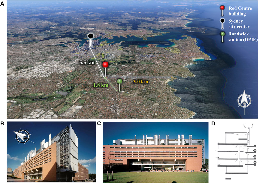
FIGURE 1. The case study: (A) geolocalization of the University Campus and the Red Centre Building (red marker) with reference to Sydney’s center to the north-west, the coastline to the east and the outdoor data reference station (see Sensor Network section); (B) North-West view of the building including the vertical shading on the western facade; (C) frontal (north) view of the building where the terracotta tiles and the solar chimneys are implemented; (D) schematics of the ventilation strategy comprised of internal passages and discharge through the solar chimneys.

The Red Centre building is particularly selected as it was constructed considering a variety of natural ventilation strategies - including cross ventilation and air updraft by solar chimneys - that aim to integrate passive environmental control and energy efficiency principles during the design stage (Figure 1D). Air-conditioning (A/C) was restricted, except for high internal load areas like computer labs, meeting rooms, studios and for occupied areas in the basement (Baird and Marriage; Baird, 2003) where A/C was provided by single-split air conditioners. In absence of A/C provisions, a number of ceiling fans was installed, proportional to the floor area. The building stretches across 6 levels, on top of basement, ground level and mezzanine, each connected to the lower levels by complex architectures of air passages aimed at verticalized exhaust air expulsion. The building is 150 m long and 15.7–19.3 m wide, with a total internal area of about 16,000 m² (Baird, 2003) and an almost perfect alignment with cardinal directions (<10° mismatch). Its strategic exposure to the north/south axis, and its limited depth along the east-west axis allows for a high proportion of natural lighting. Other passive sustainability principles include the protection of the west glazed facade with operational vertical shading devices (Figure 1B), and the localized increase in thermal mass by making use of terracotta tiles on the northern facade (Figure 1C). The southern side is typically characterized by glazed facades with louvres, while the northern side typically features twin glazing “slots” to avoid glare and sunlight overexposure.

Despite the technical adroitness and the number of awards received for sustainable design, the Red Centre building largely fails at preserving IEQ. In 2015, a post-occupancy user satisfaction survey was conducted on 30 highly sustainable institutional and commercial buildings across 11 countries (Baird, 2013). Respondents were asked to rate 45 factors on a 7-point scale, including 1) operational aspects (e.g., space use, furniture, facilities), 2) environmental aspects (e.g., temperature and gradients, humidity, air quality), 3) lighting (e.g., natural/artificial light, glare), 4) noise (e.g., source and magnitude, frequency of undesired interruptions), 5) personal control (e.g., access to HVACs controls, to windows operation, to noise source switches), and 6) user satisfaction (e.g., comfort, health, productivity). The Red Centre building ranked 27th overall, 27th in terms of comfort, 23rd in terms of health preservation, and 25th in terms of perceived productivity and was noted as being excessively cold in winter, hot in summer and noisy. Most penalties were associated with excessively intense ventilation and wind whistling across the building. The survey emphasized that, with exception of image and lighting which scored well, most other IEQ aspects were poorly addressed and ventilation was substantially misapplied.

Sensor Network

To investigate the reasons behind poor IEQ performance, a fine-grained IoT sensor network was established across the building from the basement to level 6, distributed in offices, classrooms, computer labs, studios, meeting rooms, print rooms, media rooms, and multilevel study areas. Figure 2 shows a GIS representation of room locations on different floors and sensor locations within each surveyed room. Supplementary Appendix Table A1 provides additional quantitative and qualitative information used to characterize the different rooms, including HVAC provisions (e.g., A/C units, fans), and window characteristics (e.g., facade coverage, shadings, operability). Sensor numbering in Figure 2 corresponds to that in Supplementary Appendix Table A1.

FIGURE 2

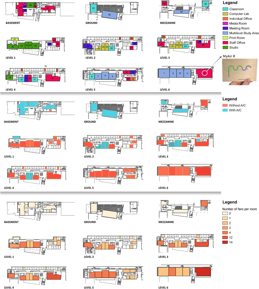
FIGURE 2. GIS representation of monitored rooms across the different levels of the Red Centre. The three colormaps correspond to room use, presence of air conditioning systems, and fans. The numbers on the maps correspond to the MyAir identification number, as reported in Supplementary Appendix Table A1.

The MyAir sensors deployed in this study represent an in-house, low-cost multi-parameter detector that includes an Arduino board with twin full-colour LEDs and three onboard sensors developed based on IoT paradigms. The sensors monitor four parameters: CO₂ (Non Dispersive Infrared sensor, T6713 Amphenol), TVOCs (metal oxide semiconductor sensor, CCS811 AMS), and T/RH (thermistor, BME280 Adafruit). All components are open source, including hardware schematics, firmware, server back-end, front-end and sensor data. The sensors were calibrated against the LST Heat Shield (ELR610M) and Aeroqual (Series 500) Portable Indoor Monitor, which are scientific grade sensor solutions for microclimate and air quality analysis. During calibration, the MyAirs returned reliable and stable measurements under a variety of thermodynamic conditions with recorded accuracy of ±0.9°C for T, ± 3.5% for RH, ± 3% for CO₂ and ±30 ppm for TVOCs. Additionally, to inform the occupants’ activities and decision making in real time, a LED-coloured indicator was added on the front side to reflect the indoor CO₂ level. The readings are sent to the real-time visualisation dashboard and stored in the cloud-based storage server (UNSW, 2021). 65 MyAir devices were originally installed in the Red Centre building in December 2018, at 1.5 m above the floor, away from doors, windows and A/C units. The sampling time was set to 15 s.

The monitoring campaign discussed in this paper represents the period between February 18th, 2019 and May 31st, 2020. This window is selected to analyse IEQ not only in a period with standard occupancy, but also the Black Summer bushfire season (peaking between November 2019 and January 2020) and the COVID lockdown period (March 31 - May 30, 2020). This extended analysis offers a unique opportunity for comparison and identification of IEQ anomalies associated with extreme natural hazards and occupancy patterns.

Within the first 2 weeks of monitoring, several sensors were deemed faulty (with regards to connection to the cloud server), vandalized, or stolen in public locations. Accordingly, compared to 65 sensors initially set up, a smaller number is used in each analysis presented, based on either having >75% readings across the whole monitoring campaign (38 sensors) or having >90% readings within comparative periods (23–42 sensors). The comparative periods last 1 month each and are hereinafter referred as 1) Term 1 (1–30 April 2019), Term 2 (1–31 July 2019), Bushfire (1–30 November 2019), and COVID-19 (1–31 May 2020). Term 1 and Term 2 indicate the academic terms with hottest and coldest outdoor conditions and are representative of standard occupancy levels. Bushfire is representative of late spring conditions exacerbated by catastrophic bushfires all around the city of Sydney. “Safer-at-home” orders were issued during this period. COVID-19 is representative of the pandemic “stay-at-home” period in autumn 2020. Supplementary Appendix Table A2 collects the list of sensors used for the analysis of each considered time period.

Over the same period, outdoor data was taken at a NATA-accredited meteorological and air quality monitoring station less than 2 km away from the Red Centre building, established by the New South Wales (NSW) Department of Planning, Industry and Environment (DPIE) network. The outdoor measurements are included to 1) investigate the indoor-outdoor inter-parameter correlations, and 2) identify which rooms were more responsive to outdoor variations.

IEQ Metrics

Here, we focus on indoor thermal comfort and air quality as metrics for IEQ. Thermal comfort is one of the most common metrics in IEQ analyses and found to be strongly correlated with occupants’ working performance and productivity (Abdul Rahman et al., 2014), health and morbidity (Quinn et al., 2014) as well as perception of indoor air quality (Fang et al., 1998).

Comfort indices customarily account for six parameters affecting human thermoregulation (air temperature, air velocity, humidity, mean radiant temperature, metabolic rate and thermo-physical properties of clothing) and are commonly calculated based on the heat balance of the human body (Potchter et al., 2018). In indoor environments, however, low wind speed and solar radiation is assumed, leading to the estimations of thermal comfort based on temperature and humidity measurements. Several temperature-humidity indices are well established internationally for indoor environments or in shade and have been extensively used in literature: the Heat Index (HI), the Thom’s Discomfort Index (DI), and the Humidex (HD). Thom’s DI fails under cold conditions, and climate-specific variants are better used when available (Moran et al., 1998; Chernev et al., 2012). HI is used operationally by the US National Weather Service (NOAA, 2021), while HD is the standard Canadian index (Government of Canada, 2021). Previous research proved that HD very often leads to the underestimation of workplace heat-related dangerousness and a poor reliability of comfort prediction when it is used in indoor situations (Alfano et al., 2011). Accordingly, in this study, we applied HI analysis for the summer (Rothfusz and Headquarters, 1990) and referred to existing thermal comfort Standards for the winter given the available microclimate data and information.

Beyond microclimatic parameters, CO₂ and VOCs are two common indoor air pollutants associated with indoor ventilation rates, SBS symptoms and health risks (Apte et al., 2000; Apte and Erdmann, 2002; Norbäck and Nordström, 2008; Gallego et al., 2011). CO₂ is a typical indirect metric of occupancy levels, amount of ventilation, and electronic appliances use, whereas VOC emissions are in the form of gases released from common furniture materials and appliances, such as wood products, photocopiers, printers and cleaning products. These compounds are extremely sensitive to both occupancy and pollution episodes, which makes them especially meaningful in comparing the control period of standard occupancy (Term 1) with natural (Bushfire) and anthropogenic (COVID-19) extremes. Besides, the locally dominating arboral genus, Eucalyptus, is a major natural polluter of biogenic volatile organic compounds (BVOCs) such as isoprene and monoterpenes, whose normal emission rate gets amplified during bushfire events (Bolan, 2020).

In this study, we adopted standardized thresholds to identify different health risk levels for each of the considered IEQ indexes. The United States National Weather Service classifies HI into four categories including Caution, Extreme Caution, Danger and Extreme Danger, associated with a range of potential health effects under prolonged exposure (Nws, 2021). Indoor CO₂ is classified based on commonly-used international guidelines, into 6 categories ranging from Good to Hazardous, (Saad et al., 2017). The impacts on cognitive performance and health (e.g., headaches, dizziness, vomit) soars when CO₂ reaches 1,000 ppm (Loh and Andamon; Satish et al., 2012), which is the commonly accepted threshold for indoor CO₂ concentration in literature and regulations (Daisey et al., 2003; ANSI/ASHRAE, 2016; Abcb, 2018). Finally, the German Federal Environmental Agency has expanded the World Health Organization (WHO) guidelines for TVOCs classification (World Health Organization, 2000) to incorporate 5 classes of increasing health impact from Excellent to Unhealthy (Umweltbundesamt, 2007). The different classes and their corresponding class limits are listed in Table 1 below.

TABLE 1

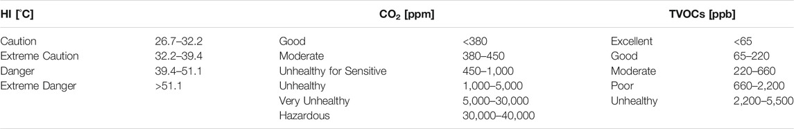
TABLE 1. IEQ Classification based on Heat Index and measured pollutants.

Results

General Descriptive Analysis

Figure 3 depicts all measured variables across the 15-months monitoring period, based on available MyAir sensors (coloured dots in the background). The daily means of all sensors in the occupied hours (9am–6pm) are overlapped as black lines with the yellow shade indicating the standard deviation range. The grey vertical blocks in the background identify weekends, while the arrow-like annotations on top of the figure locate the comparison periods across the timeline. For pollutants, the health classification is displayed as well in the form of dashed horizontal lines and is labelled according to Table 1. For T and RH, the blue lines with diamond-shaped markers denote outdoor measurements. Table 2 complements the trends in Figure 3 by reporting general statistics on minima, means and maxima among the whole set of MyAir sensors, considering the 15-min time-averaged data.

FIGURE 3

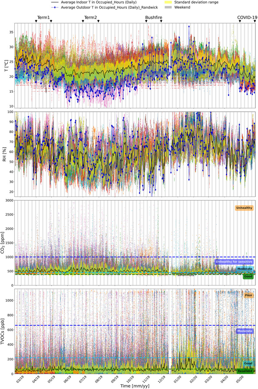
FIGURE 3. Time trends of temperature, relative humidity, CO₂ and TVOCs between February 2019 and JuneMay 2020. Outdoor measurements are taken from the DPIE station located in Randwick. A blackout period occurred between the 14th and the December 21, 2019, causing all MyAirs to stop recording.

TABLE 2

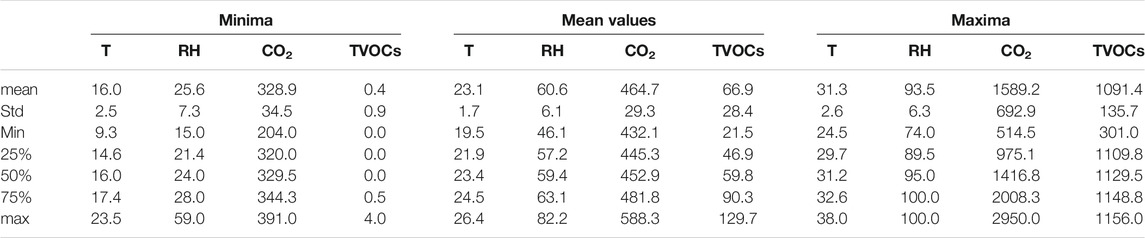
TABLE 2. Statistical analysis across all MyAir sensors and over the entire observation period (Feb 2019–Jun 2020).

On average, the hottest and coldest months in the indoor spaces were March (average of 30.2°C) and August (average of 13.6°C), yet extreme hot days also occurred in April. The most humid time of the year was January, February, and November (average of ∼85%), while the driest occurred between June and August (average of ∼37%). CO₂ and TVOCs typically hit higher concentrations in summertime (November-December) and October-November, and reached lower concentrations in October and April, respectively. Over the period of analysis, the hourly mean outdoor T was 18.1°C, hitting a maximum of 41.7°C in the middle of the bushfire season (late January 2020) at peak hours, and a minimum of 4.2°C in mid-winter (August 24, 2019) in the early morning. The corresponding values in terms of relative humidity were 70.3%, 100% and 7.3% with both maximum and minimum occurring between November and December 2019, in the morning and afternoon respectively. These trends impacted on different rooms in the building in a distinct way.

The absolute maxima of indoor T, RH, CO₂, and TVOCs observed in sensor measurements were 38.0°C, 100%, 4,688 ppm, and 1,156 ppb, respectively, and were recorded over occupied hours on workdays. Notably, the T maximum was observed in the morning during summer term, while the CO₂ maximum was seen in March 2020 right before the beginning of COVID-19 lockdown at about 3pm. Both RH and TVOCs maxima were measured on the same day (Aug 12, 2019) between 5 and 6 pm. T, RH and TVOCs maxima were all measured in individual offices, located on Level 2 (T) or Level 4 (RH and TVOCs). In sharp contrast, the CO₂ absolute maximum was recorded in a classroom located on the mezzanine. All maxima occurred in north-oriented rooms featuring no A/C. The maximum averages were 27.8°C, 76.3%, 675 ppm and 109 ppb, with all values (but RH’s) higher than measurements averaged for the entire week (including weekends and nights). The maximum of average T (for all sensors) was measured in an individual office on Level 2, facing north, whereas the maximum RH mean was measured in a studio on Level 1, facing south. In both cases, no A/C was in use. Conversely, air-conditioned rooms were conducive to higher average pollutant concentrations: the maximum CO₂ mean was recorded in the print room on Level 1, while the maximum TVOCs mean was recorded in a staff office in the basement.

Interestingly, the room use associated with most absolute maxima (individual offices) was also associated with most absolute minima, at 10.3°C, 17.3%, 232 ppm and 0 ppb. Indeed, RH, CO₂ and TVOCs minima were all measured in individual offices on different levels (2 north-side,4 north-side and 5 south-side respectively), with no A/C. The absolute T minimum was reached in a classroom located on the ground floor, western-oriented and air-conditioned, and not in colder months. Minima in T and CO₂ were aligned in time as both occurred in March 2020 early afternoon, but even more aligned were the minima in RH and TVOCs both recorded on June 24, 2019 at around 5:30 pm. The minimum averages were 19.3°C, 43.6%, 432 ppm and 23 ppb, with all values (but RH’s) higher than those measured for the entire week. The minimum T and RH averages were measured in non-air-conditioned rooms on Level 2, the former in a south-exposed classroom, and the latter in a north-exposed individual office. Conversely, both CO₂ and TVOC minimum averages occurred in meeting rooms, located in the basement and Level 2 and featuring A/C and ceiling fans respectively.

Overall, the absence of an air-conditioning system was conducive to greater indoor extremes. North-exposure was associated with both T maxima and maximum means. In the southern hemisphere, north-facing windows receive twice the winter Sun than east and west facing windows, allowing light and warmth into the building. Relative humidity peaks are associated with the availability of moisture and latent heat which depends on people and their activities, construction materials, and presence of cold surfaces, water sources (e.g., kitchens), and rain penetration. Windows, walls, and doors that lack proper insulation and tightness and have limited exposure to Sun radiation are common cool surfaces. This explains why maximum RH mean levels were measured in high-occupancy rooms potentially featuring a variety of moisture sources (studios), located close to the ground and facing south, where shading from neighbouring elements (e.g., building, trees) is most effective and sunlight penetration is weakest. In terms of room use, individual offices exhibit a distinctive behaviour. Indeed, they represent the smallest rooms on average and thus accumulate heat, moisture, and pollutants more easily and more promptly. Having a small air volume with one longitudinal, highly transmitting windowed side, these rooms respond very quickly to outdoor variations too. On the other side, as one single person is typically the greatest source of all measured parameters and controls all ventilation adjustment actions, these rooms are extremely susceptible to occupancy patterns and comfort-restoring actions, which explains the variability range. Maximum means in pollutants concentration are associated with the room use and ventilation rates, which justifies the poor air quality in print rooms and the accumulation in the basement. Cleaning and renovation activities also occurred during the monitoring period which are mostly associated with TVOCs peaks.

Site Characterization

Room use, level, orientation, HVAC provisions, and window extent and operability are key actors in arbitrating IEQ levels across an educational building. As such, the following analysis is focused on spotting spatial heterogeneity and inter-parameter associations conditioned over room characteristics. The analysis is performed using the hourly dataset over occupied hours, focusing on workdays only.

Role of Room Use Under Standard Occupancy

To get an understanding of how room use is associated with higher or lower IEQ levels, we focused on the time period with standard occupancy and warm-to-hot outdoor conditions (Term 1). Figure 4 shows a combined box and swarmplot of hourly and daily averages respectively, grouped by room use. Only sensors with more than 90% data over the studied time interval are considered (Supplementary Appendix Table A2). All room types are represented here except for the print room, which was monitored by only one sensor and will be discussed later. The average is further displayed as a green horizontal line and used to order the boxplots (decreasing mean).

FIGURE 4

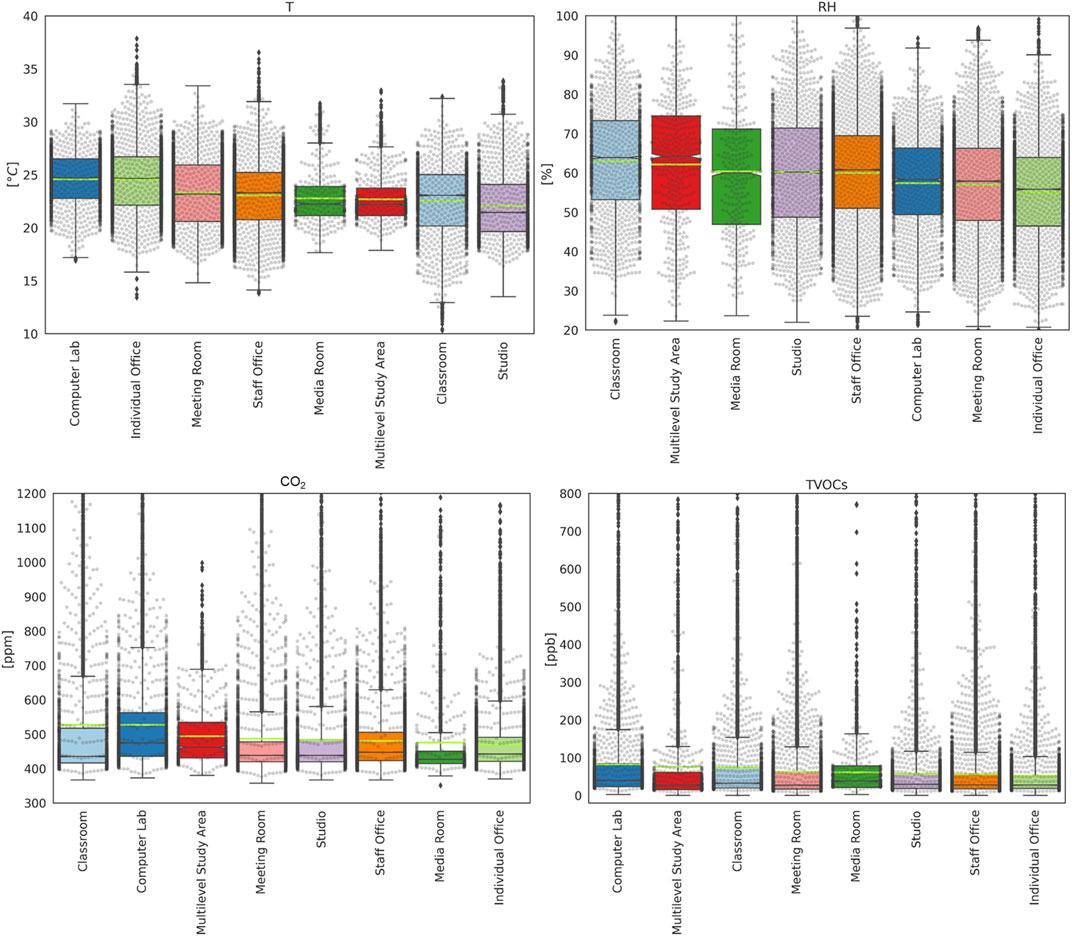
FIGURE 4. Different IEQ behaviour across different room types under standard occupancy (Term1). The y-axis limits are adjusted for a better visual comparison of results. The swarmplots show daily mean observations and complement the representation of the underlying hourly distribution (boxplots).

During Term 1, rooms exhibited distinct behaviors, summarized in Table 3. Computer labs and individual offices exhibited the highest T mean (24.6°C). High local production of heat from local appliances, typical elevation, exposure, presence of partially glazed facade and absence of solar shadings are major triggers and further explain why computer labs, together with classrooms, exhibit the highest mean CO₂ (527.0 ppm) and TVOCs (82.0 ppb) concentrations with significant extreme episodes. As observed in General Descriptive Analysis section, individual offices tend to experience high variability and the most extreme high-temperature events. This is demonstrated by the wide interquartile (IQR) range (4.6°C) and the dense cloud of recordings above 26.7°C. Reasons include the low air volume and the presence of portable heating devices which also result in drier air (mean of 55.0%, typical range = 46.6–64.0%). In terms of pollutants, individual offices had the lowest CO₂ and TVOCs means (470.5 ppm and 51.7 ppb), mainly due to lower internal gains. While heat cannot be efficiently controlled due to the considerable solar gains (due to exposure, insufficient shading provisions), the combination of operable windows and ceiling fans proved sufficient in limiting the accumulation of pollutants. Meeting rooms experienced fairly comfortable thermo-hygrometric and pollution levels, likely caused by the irregular occupancy pattern, scattered in time and short-lasting. Temperatures were lower compared to individual offices and computer labs, yet higher than rooms having even higher occupancy density (e.g., classrooms) but better ventilated. This also explains the amount of outliers in CO₂ and TVOCs charts, with both reaching unhealthy levels during closed-door meetings. In staff offices (encompassing shared and open-plan areas), the mean T is at 23.1°C, and the mean RH around 60.0% due to the local presence of latent heat sources. While very limited health-threatening events were recorded in terms of CO₂, frequent extreme TVOCs episodes occurred which can be imputed to major renovations, re-painting and cleaning activities. The media room (a multipurpose space outfitted for video-making and media releases) exhibited limited temperature variability (within ±1.5°C of the mean 22.8°C) but comparatively high RH (46.9–71.1%). TVOCs never crossed unhealthy levels and CO₂ very rarely. The CO₂ mean (475.6 ppm) was the second-to-last across all room uses. This pattern is mostly related to its sporadic and time-framed use. Multi-level study areas, located across Level 5 and 6, exhibited medium-low T levels (mean of 22.7°C), yet high RH, CO₂ and TVOCs (means of 62.1%, 493.8 ppm and 75.4 ppb). Despite benefitting from both horizontal and vertical cross ventilation, this proved sufficient only at removing heat, but not moisture and pollutants which tended to accumulate on lower levels, gathering the contributions of multiple floors. Further, these rooms are typified by non-openable fully glazed facades, thus limiting the intake of outdoor air. Classrooms were fresher (with T typically in the 20–25°C range) and experienced limited TVOCs accumulation (levels below 73.2 ppb) thanks to their south-exposure and operable shading provisions, however mean CO₂ was the highest (527.3 ppm) and frequently crossed the unhealthy threshold and high humidity levels (mean of 63.0%) occurred, both likely caused by the high internal gains. Studios exhibited the lowest T levels (mean of 22.1°C), and a relatively comfortable RH range (50–71%). However, temperature levels were skewed towards the upper quartile with extremes over 30°C, likely caused by the presence of fully glazed facades, although south-exposed. CO₂ could surpass the unhealthy threshold, while TVOCs stayed within moderate levels. Because CO₂ is heavier than air, it sinks to the lower floors across the building. Almost all studios are located on Level 1 and feature no A/C that could extract the excess CO₂ or facilitate its removal.

TABLE 3

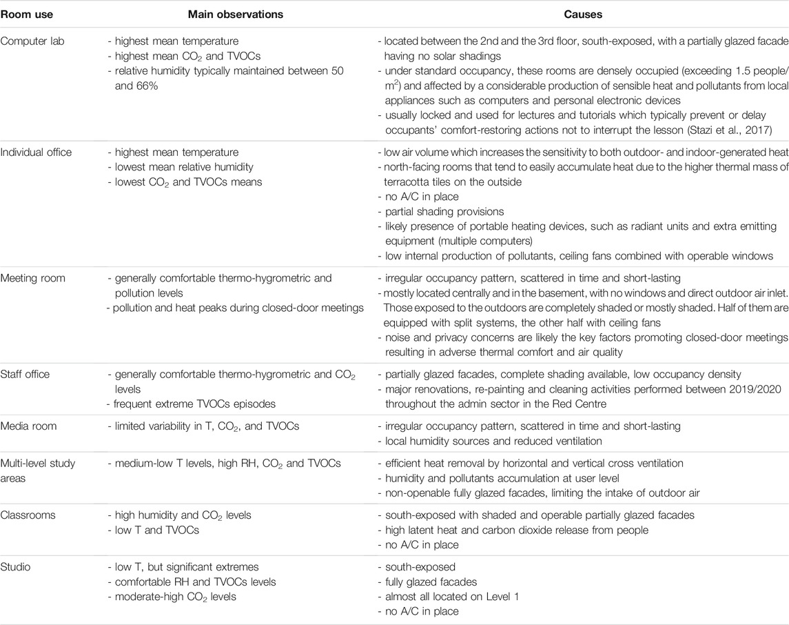
TABLE 3. Typical IEQ pattern per room use under standard occupancy.

The effect of seasonality is explored in Figure 5, where the warmest (Term1) and coldest (Term2) periods of standard occupancy are compared, based on sensors having more than 90% of data in both the time windows (Supplementary Appendix Table A2). During Term 1, the outdoor temperature was 18.9 ± 3.3°C with a maximum of 27.8°C and a minimum of 9.8°C. Relative humidity ranged within 75.9 ± 14.9%, reaching a maximum and minimum of 98.6 and 23.4%, respectively. During Term 2, the outdoor temperature was 6° lower (13.0 ± 3.3°C) while relative humidity was nearly 13% lower on average (62.5 ± 18.1%). The outdoor temperature is consistently lower than indoor throughout the whole year. This is attributed to the weather station location (green, open area, closer to the coastline) and the internal gains.

FIGURE 5

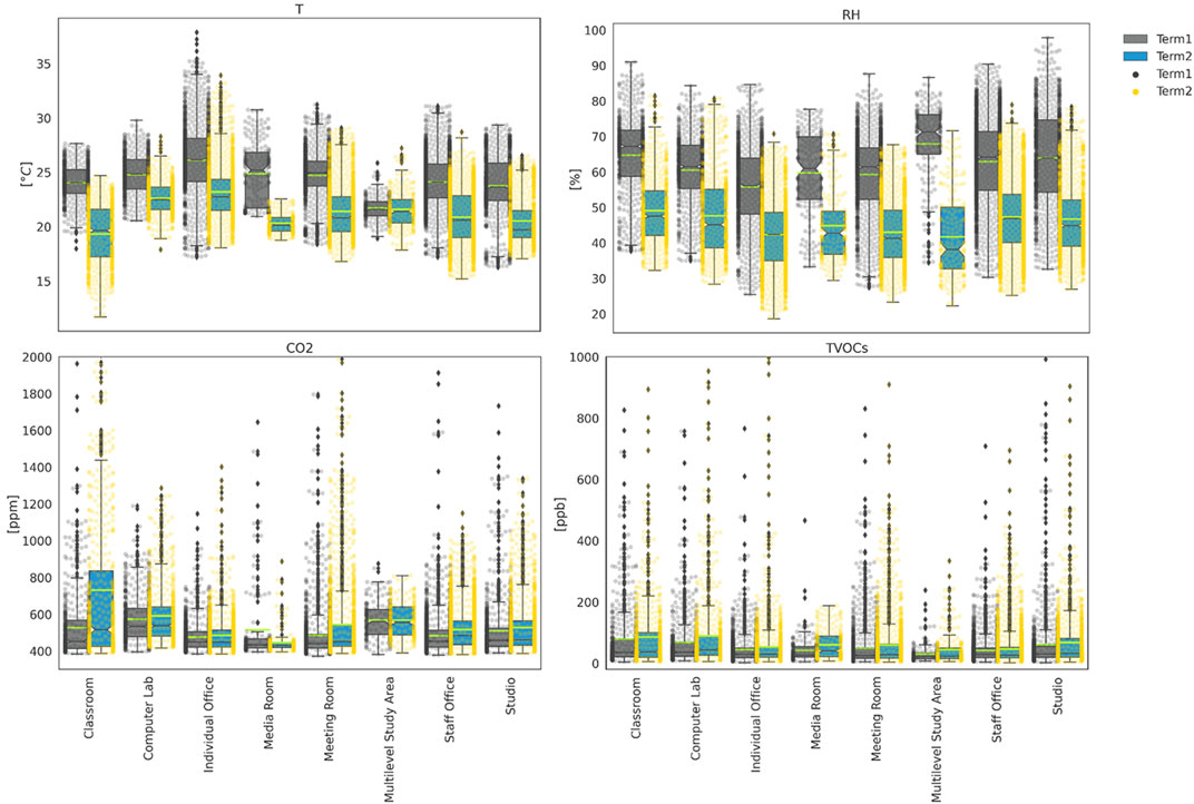
FIGURE 5. IEQ behaviour across different room types: comparison between warm and cold standard occupancy periods. The y-axis limits are adjusted for better visualization. The swarmplots show all mean observations, on hourly scale, and complement the representation of the underlying distribution.

In both Terms, the indoor temperature was 1–2°C warmer and <5% more humid as compared to outdoor conditions, due to high thermal transmittances, extensive glazed surfaces and emission of latent heat from occupants. Some exceptions occurred. The indoor temperature difference was much more limited in computer labs and multilevel study areas, where the internally-generated heat outweighed the heat loss through the building envelope and to unconditioned indoors. Classrooms could reach significantly lower temperatures having extensive shaded windowed sides on the north facade. The relative humidity difference was close to 15% on average, with multilevel study areas touching a major gap of more than 20%. Generally speaking, the humidity levels tended to equalize across different rooms in the colder Term with medians within a 5% range, compared to more than 10% in Term1. The reasons are to be found in the extensive use of portable heaters that efficiently dried the air down to a RH of about 45% on average. As for CO₂, mild discrepancies are observed between Term 1 and Term 2, which entails that CO₂ levels are not governed by seasonal cycles. A standalone behaviour is that of classrooms where considerably higher CO₂ levels are recorded. The reason is likely behavioural: while classes tend to start and go on with open windows during the warm Term, this is hardly the case during wintertime, when windows and doors are kept closed to maintain the warmth inside. As such, people’s respiratory emissions were not dispersed as efficiently as in Term 1 and accumulated over unhealthy levels, with the mean being nearly 200 ppm higher. Finally, the offset in terms of TVOCs was negligible regardless of the room use.

The print room on Level 1 lacked enough data in Term 1, however its IEQ pattern is of special interest due to a combination of aggravating factors. Beyond the presence of printing devices, the room is exposed to the outdoors on three sides, with the northern being the longest. A single unshaded window of about 1 m² stretches along the western side. No cross ventilation occurs given that the door is spring-loaded to automatically close and even though air conditioning is in place, ventilation is very limited. The sensor continuously recorded from the April 14, 2019 on, as such a month period up to the May 15, 2019 was used to characterize its behaviour in Term 1. The results over occupied hours and workdays only are summarized in Table 4. Temperature and TVOCs stayed very low, at levels comparable to those of multilevel study spaces in Figure 4, while relative humidity stayed high at levels comparable to those of the media room. The most critical observation is made in CO₂ concentration: the average exceeded 937.8 ppm which is 410 ppm higher than the highest level recorded by any other room type during the same period, with an IQR of 482.4 ppm which is 10-fold that of other rooms. This suggests that the average conditions inside the print room are unhealthy for the sensitives and cross the health-risk threshold of 1,000 ppm more than 25% of the time. Only a negligible improvement is recorded in Term 2. This calls for major redesign measures in order to meet minimum liveability levels.

TABLE 4

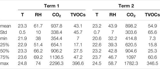
TABLE 4. Statistical analysis for the print room over Term 1 and Term 2.

Proclivity to IEQ Deterioration

In this section, statistical analysis is performed to identify which rooms were more prone to seasonal IEQ extremes and criticalities. Only sensors having more than 90% recordings over each season were included (Supplementary Appendix Table A2). Upper and lower outliers are those exceeding the 75th percentile or falling below the 25th percentile by 1.5 times the interquartile range. For each sensor and each parameter, the percent occurrence of upper and lower outliers was computed. Figure 6 is a summary GIS representation of the 4 most critical extremes in terms of IEQ deterioration: summer upper outliers for T and TVOCs, winter lower outliers for RH, and winter upper outliers for CO₂. It allows immediate visualization of the locations most prone to extreme conditions.

FIGURE 6

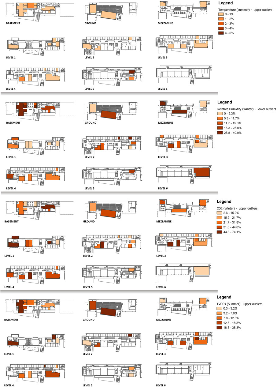
FIGURE 6. GIS localization and categorization of rooms according to their proclivity to extreme events. From top to bottom: occurrence of summer upper T outliers, winter lower RH outliers, winter upper CO₂ outliers, and summer upper TVOCs outliers (percent time). Upper and lower outliers are those exceeding the 75th percentile or falling below the 25th percentile by 1.5 times the interquartile range.

Most high extreme temperature events occurred in summertime, with 22% of the sensors recording outliers. The maximum percent occurrence was 4.5% in the north-oriented meeting room at Level 5. Comparatively, 16.7, 7.9, and 12.1% of the sensors recorded outliers in autumn, winter, and spring with a maximum of 3.6% of the time. Lower outliers mostly occurred in springtime with 36.4% of the sensors measuring up to 28% of the time below the threshold. Most extreme dry events took place in winter, with 78.9% of the sensors measuring outliers. In an individual office on Level 2, extreme dry events occurred for 41% of the time, likely caused by an overuse of portable heaters. Dry events were recorded at almost all locations also in other seasons but rarely surpassed 10% of time. Conversely, extreme humid episodes concentrated in summertime but over limited time periods (<1%). CO₂ extreme events exacerbated in wintertime, with 84.2% of the sensors recording poor air quality, typically for more than 20% of the time. As mentioned in Role of Room Use Under Standard Occupancy section, the print room recorded the worst conditions with an astonishing 74.1% of the time under extreme CO₂ levels. Further a computer lab on Level 2 and a studio on Level 1, both south exposed, recorded outliers for more than 50% of the time. Almost all sensors recorded extreme CO₂ levels in any other season, however the time coverage was typically lower than 20%. In terms of TVOCs, summer was by far the worst season: all sensors recorded outliers and most for more than 10% of the time. The greatest time coverage was 38.3% and occurred in a centrally located staff office in the basement.

The above analysis suggests that the most critical conditions to moderate not to pose a risk on occupants’ health and productivity are wintertime CO₂ levels.

Heat Index

Heat stress occurs out of the boundaries of the zone of homeothermy, namely the range of environmental conditions in which humans maintain heat balance and thereby a steady core temperature by minimal thermal adjustments (comfort zone) or mild thermoregulating reactions like shivering and sweating (Lacetera et al., 2003). Here, the hottest average indoor temperatures were recorded in March 2019, while the highest extremes were recorded in April 2019. Consequently, the heat index analysis was performed contemplating both months. Figure 7A shows the result, based on sensors having more than 90% of data only (coloured dots in the background). The daily means in the occupied hours (9 am–6pm) are overlapped as salmon-shaded, red lines with the shade indicating the one standard deviation span. The health classification thresholds are displayed in the form of dashed horizontal lines and labelled according to Table 1.

FIGURE 7

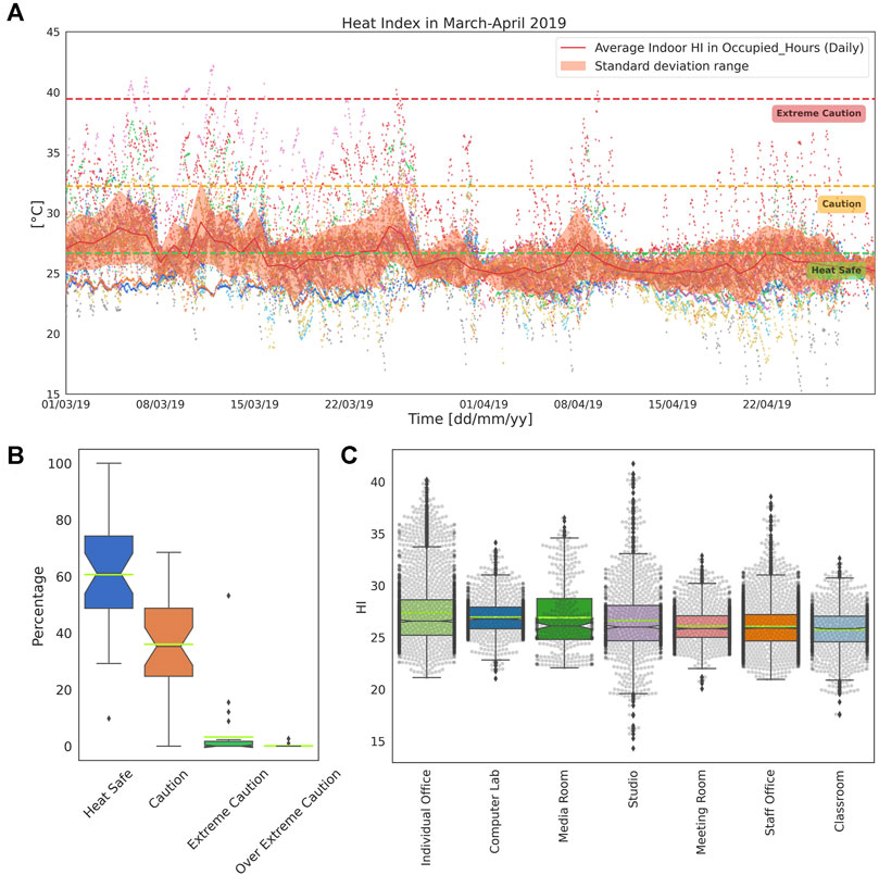
FIGURE 7. Heat index analysis: (A) time trends between March and April 2019; (B) boxplot of occurrences under different health risk levels and (C) box and swarmplots of HI level broken down by room type, both showing mean observations, on hourly basis.

The mean HI ranged between 24.2 and 32.2°C, with the lower limit measured in a north-oriented studio in the basement and the upper limit in a north-oriented individual office on Level 2. The maximum HI ranged between 26.4 and 41.7°C with the absolute peak recorded in a centrally located studio in the basement. Conversely, the minimum ranged between 14.3 and 24.5°C with the absolute low observed again in the north-oriented studio in the basement. Maxima typically occurred in the 12–1 pm and 3–4 pm windows. In contrast, minima mostly occurred in the morning. Figure 7B shows the percent time spent into increasing levels of health risk in the form of a boxplot. Heat safe conditions were largely dominant, with two offices in the basement never experiencing any sort of risk (possibly due to A/C access). The lowest percent time in heat safe conditions (9.8%) pertains to the individual office on Level 2 typified by extremely dry air (which also scored the maximum percent time in the Extreme Caution zone, 53.2%), followed by 29.2% in a west-oriented studio on Level 4 (that also scored the maximum percent time in the Caution zone, 68.5%). All rooms having significant percentages (9–16%) in the Extreme Caution zone and even above it are located in the basement. We observe that rooms located in the basement may experience the best and worst HI conditions depending on the efficiency of air conditioning and on the ability to dissipate excess humidity. In terms of room use (Figure 7C), individual offices hit the worst HI conditions, having mean above the heat-safe upper threshold (27.4°C versus 26.7°C) and 75th percentile close to the Caution threshold. Computer labs follow closely with mean HI at 27°C, but much lower variability (IQR equal to 2.1°C versus 3.4°C) and much less frequent extremes. The media room in the basement and studios also exists on the borderline of heat safe conditions (mean of 26.9 and 26.6°C) with HI distribution significantly skewed towards upper values. As for the print room whose IEQ was deteriorated by CO₂ levels, this analysis reveals how major redesign measures are required for individual offices, computer labs, studios, and media rooms in order to maintain heat safe conditions, on average. Health-preserving strategies should target both temperature and humidity as both contribute to establishing heat stress conditions in the warm season (compare Figure 4). Meeting rooms, staff offices and classrooms behave very similarly with mean levels in the 25.9 ± 0.2°C range. Meeting rooms exhibit the least IQR (2.1°C), comparable to that of computer labs. Maxima reach or slightly exceed 40°C, thus trespassing the Extreme Caution threshold. Minima typically stay around 20°C. Studios show the widest variability by far, ranging between the absolute minimum (14.3°C) and the absolute maximum (41.7°C). Much safer conditions pertain to classrooms, whose variability range is completely contained within the Heat Safe bounds, to the benefit of students’ productivity and comfort.

Inter-parameter Correlations and Key Variables

In this section, the correlation among indoor and outdoor parameters is investigated by means of Mutual Information (MI) analysis. MI is a statistical metric that measures the degree of “shared information” between time series x, y by quantifying the difference between marginal and joint entropies (Fraser and Swinney, 1986; Cellucci et al., 2005; Frenzel and Pompe, 2007). It is typically normalized to range between 0 and 1, where 0 connotes mutual independence, and expressed as:

$MI\left(X;Y\right)=\sqrt{1-exp(-2\cdot I(X:Y)}(1)$

where I is calculated based on the probability density p as follows:

$I\left(X;Y\right)={\displaystyle \underset{R^2}{\int }p\left(x,y\right)log\left(\frac{p\left(x,y\right)}{p\left(x\right)p\left(y\right)}\right)d\left(x,y\right)}(2)$

MI is a powerful correlation measure for exploratory analysis of variable pairs for three main reasons: 1) it captures both linear and non-linear relationships, being equivalent to Pearson correlation in the linear case, 2) it can be conditioned on a third, possibly multidimensional, variable, being analogous to partial correlation, and 3) it is invariant under monotonic transformations of variables, including linearization. Conditioned MI returns the degree of association with the effect of a given controlling variable removed. For instance, conditioning over the day of the year removes the effect of seasonal cycles. MI has been applied in atmospheric science (Zaidan et al., 2018, 2019) and urban analysis (Li et al., 2014; Ryu et al., 2018; Ulpiani et al., 2021), revealing strong non-linear associations especially when wind-related and air quality parameters are concerned. In this study, we applied MI correlation to look for the inter-parameter associativity under standard occupancy (Term 1) via k-nearest neighbour search. The correlation matrices for the rooms where maxima MI were computed are shown in Figure 8. We also investigated if and which site-specific parameters (e.g., altitude, orientation, A/C provisions, window types and shadings) govern the strength of correlation by applying conditional MI (Laarne et al., 2021). We included outdoor parameters measured at the DPIE station in Randwick, which comprised wind speed (ws), wind direction (wd) and four outdoor pollutants (NO₂, O₃, PM₁₀ and PM_2.5), outdoor temperature (T_out) and relative humidity (RH_out). Supplementary Appendix Table A3 collects the list of parameters that were significantly correlated to the four MyAir measurements. The significance threshold was set to 0.5, namely midway between mutual independence and full correlation.

FIGURE 8

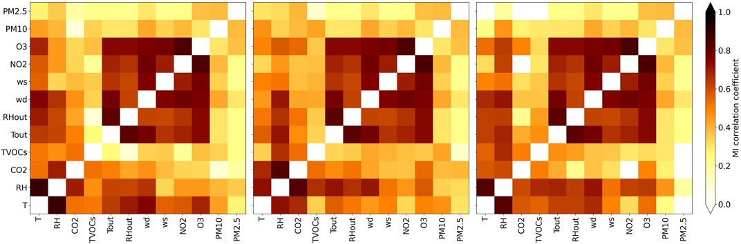
FIGURE 8. Inter-parameter correlation coefficients for MyAir #59, #51, and #25 (shown respectively from left) where maximum MI correlations were observed.

Relative humidity was, by far, the most correlated parameter, followed by temperature, CO₂ and TVOCs. The absolute maximum correlation coefficient for T was with RH and reached 0.88. It was recorded in a studio in the basement. Temperature tended to be most correlated to RH (86.0% of cases), T_out (7.0%) and CO₂ (7.0%) while it exhibited mild correlation with all other outdoor parameters and with TVOCs. In terms of RH, the absolute maximum correlation coefficient was the same as for T, measured in the basement studio. Relative humidity was typically correlated with T (79.1% of cases), equally followed by CO₂ and wd (9.3%) and then by RH_out (2.3%). Indeed, in Sydney, the wind direction dictates whether humid fresh air is entrained by the sea breeze from the east or dry warm air is advected by desert winds coming from the western fringe. This dualism has been largely investigated and governs the magnitude and spatial heterogeneity of urban heat island and outdoor heat stress (Santamouris et al., 2017; Yun et al., 2020). As for CO₂, the absolute maximum correlation coefficient was with RH and reached 0.83. It was recorded in an air-conditioned, west-exposed staff office on the mezzanine. CO₂ tended to be most correlated to RH (74.4% of cases), T (20.9%) and both T_out and TVOCs equally (2.3%). A strong linear and positive correlation between carbon dioxide and relative humidity was also found in other naturally ventilated school buildings elsewhere in the world (Lazović et al., 2016). Finally, the absolute maximum correlation coefficient for TVOCs was with RH and reached 0.67. It was recorded in a non-conditioned, north-oriented individual office on Level 3 that underwent extensive cleaning during the time of observation (MyAir #25). TVOCs were most typically correlated with CO₂ levels (34.9% of cases) and RH (32.6%), but in some cases significant correlation was found with T (16.3%), wd (7.0%) and outdoor T, ws, NO₂, O₃ parimerito (2.3%).

Floor level, orientation, room use, air volume, A/C and ceiling fan provisions, cross ventilation, type of windows, level of shadings and windows operability (refer to Supplementary Appendix Table A1) were codified and included in the dataset to verify whether knowing the room characteristics could lead to stronger associations and thus better predictability. We iterated across the different conditional parameters and calculated the difference in correlation coefficients between conditional and unconditional matrices. Interestingly, only the floor level was associated with higher correlation coefficients. The average increase was 0.09. Above average increments are those in the mutual correlation between T-CO₂ (+0.17), RH-CO₂ (+0.15), RH-TVOCs (+0.15), T-RH (+0.14), T-wd (+0.14), T-ws (+0.11), T-T_out (+0.11), and T-NO₂ (+0.10). Hence floor level is a major trigger for inter-parameter associations, especially in terms of pollutants. Since CO₂ and TVOCs are heavier than air, they travel all the way down from the upper levels to the ground. At the same time warmer, drier air tends to move upwards convectively, especially in naturally ventilated buildings provided with vertical air communication. This explains why the strength of correlation between thermo-hygrometric and air quality parameters significantly depends on the elevation.

Weather Extremes and Occupancy Anomalies

This section is dedicated to the impacts of microclimatological and occupancy anomalies on IEQ preservation by comparing the control period of standard occupancy (Term 1) with the Bushfire and COVID-19 subsets, respectively. The analysis is conducted by considering the records of sensors having more than 90% data in the paired time windows (Supplementary Appendix Table A2).

Figure 9 shows the impact of 2019/2020 Black Summer, during which hundreds of bushfires ravaged the urban fringe causing extreme pollution, heat waves and droughts. The multiple microclimatic impacts in the city of Sydney have been analysed elsewhere and include 1) health-threatening PMs accumulation due to long-transport mechanisms and complex interactions between prevailing and local winds, 2) strongly attenuated UV radiation and radiative forcing impairment, and 3) exacerbated urban heat island intensity and absence of cool island events (Ulpiani et al., 2020). In November 2019, a dense plume of smoke blanketed the city and safer-at-home orders were put in place, thus altering standard occupancy patterns. The outdoor temperature was 19.7 ± 4.0°C (higher than Term 1 by less than 1°C) with a maximum of 35.5°C and a minimum of 10.3°C. Relative humidity ranged within 63.9 ± 21.7% (lower than during Term 1 by more than 10% and much more fluctuating), hitting a high of 96.1% and an extreme low of 7.3%. These trends were closely reflected indoors, although extreme events were all strongly exacerbated. The following exemptions stood out. Computer labs are electronically locked thus acting as hermetically sealed sinks for heat, moisture and pollutants under periods of unoccupancy. Furthermore, extra heat may have also been released by remotely controlled computers as coarse dust from the bushfires amassed. Computer overheating is most commonly caused by the heat sink and fans being clogged with dust and debris. Indeed, the mean T was 4.0°C above the mean of most other rooms and was 1.0°C above the mean in Term 1. Meetings, conferences, and gathering stopped during the bushfires critical phase, thus causing a significant decrease in internal heat gains in meeting rooms as mirrored both in terms of sensible (T) and latent (RH) heat balance. The T mean was 0.5°C lower than in Term 1, and the 25th percentile was 21.3°C, 2.5°C less than in Term 1. A standalone behaviour is that of the media room in the basement, where humidity equalled Term 1 levels while temperature dropped, suggesting intense evaporative cooling. The T mean and maximum, 22.4 and 24.4°C respectively, were nearly 2.4 and 6°C less than in Term 1. The reasons for this specific trend require further investigation and might have been caused by A/C failures and water leakages.

FIGURE 9

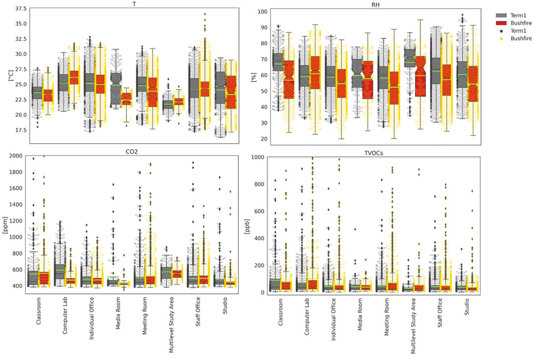
FIGURE 9. IEQ behaviour across different room types: comparison between warm standard occupancy period and bushfire. The y-axis limits are adjusted for a better visual comparison. Boxplots and overlapped swarmplots show mean observations, on hourly basis during occupied hours and workdays only.

In terms of pollutants, very interesting and distinctive patterns emerge in the comparison with Term 1. CO₂ levels dropped everywhere caused by the altered occupancy pattern. The maximum offset was again recorded in computer labs and amounted to −122.1, −115.9, and −336.4 ppm in terms of mean, IQR, and maximum, respectively. The following largest mean decrease pertained to the media room and the multilevel study areas, hitting −87.8 and −18.5 ppm respectively, with multilevel study areas showing also a significant drop in IQR and absolute maximum (−51.3 and −130.9 ppm). The reduction in means was around 5–20 ppm also in the other room types, but milder in terms of IQR and maxima. The greatest drops were recorded in rooms with high standard occupancy density (e.g., computer labs, classrooms) or receiving the contributions from multiple floors (multilevel study areas), as those were most impacted by the reduced flow of people. In sharp contrast, TVOCs increased everywhere because of biogenic emissions from biomass burning. The offset with respect to Term 1 was greatest in computer labs, multilevel study areas, and meeting rooms, reaching a maximum of 30.0, 14.5, and 58.9 ppb (mean, IQR and maximum) in computer labs. The increase in meeting rooms was comparable (26.7, 17.1, and 263.3 ppb), followed by 23.1, 23.5, and 668.7 ppb recorded in multilevel study areas. These rooms remained locked with no A/C during the safer-at-home orders and thus could not disperse air pollutants as efficiently as during standard occupancy. Smart logics should be put in place to control the A/C and door opening/closing cycles in electronically operated rooms of these types to avoid generating highly health-threatening indoor environments during bushfire events. Such results suggest an urgent need to prioritize building air tightness improvement, appropriate filtration techniques, and emergency strategies to expel excess dust towards future-proof buildings in Sydney and similar regions in the world, as also stressed elsewhere (Rajagopalan and Goodman, 2021).

The role of occupancy levels and patterns emerges even more vividly when comparing Term 1 with COVID-19 lockdown period, as displayed in Figure 10. In May 2020, the outdoor temperature was 14.9 ± 3.3°C (exactly 4°C lower than during Term 1) with a maximum of 25.5°C and a minimum of 7.6°C. Relative humidity ranged within 69.1 ± 17.1% (less than 10% lower than during Term 1), hitting a high of 96.2% and an extreme low of 29.1%. While during Term 2 the outdoor T offset with respect to Term 1 was mitigated by 1–2°C indoors, during the lockdown it got amplified in most room types by about 0.5°C. Statistically significant gaps were recorded everywhere, with reductions in the 75th percentile reaching 7°C under the lockdown, given the concerted fall in heat gains from both people and equipment. The only exception to this pattern is represented by multilevel study areas whose temperature stayed low in Term 1 too. Interestingly, the absence of people flattened out the differences across room types with all T means lying within a 1°C range across 20°C. This indicates that occupants and their actions (including central A/C or portable devices activation, windows/doors opening and closing) are pivotal in driving room-specific average temperature levels. In sharp contrast, the humidity levels in Term 1 and during the lockdown show marginal differences (<5% for almost all room types) as the loss of latent heat was largely compensated by higher relative humidity under lower temperatures. This also explains why the gap was especially narrow in studios and especially wide in multilevel study areas.

FIGURE 10

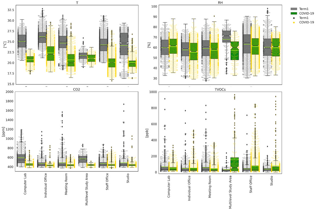
FIGURE 10. IEQ behaviour across different room types: comparison between warm standard occupancy period and COVID-19 lockdown. Boxplots and overlapped swarmplots show mean observations, on hourly basis during occupied hours and workdays only.

Similar to the bushfire period, CO₂ levels dropped everywhere. The maximum offset was again recorded in computer labs and reached −138.7, −136.8, and −445.3 ppm in terms of mean, IQR and maximum, respectively, which closely resemble the values recorded during the bushfire when the labs were closed as well. The following largest decrease pertained to multilevel study areas, whose corresponding drops amounted to −130.8, −69.2, and −359.8 ppm larger than during the bushfire as a result of the complete absence of people. The reduction in means was around 30–40 ppm also in the other room types, but milder in terms of IQR and maxima. It is thus confirmed that greatest drops occur where the occupancy density is typically higher or where multiple floors are interconnected. Looking at TVOCs, the pattern is less clear, with most room uses showing negligible changes. The only rooms that experienced significantly higher TVOCs were multilevel study areas, staff offices and studios. Notably, the offset with respect to Term 1 reaches a maximum of 133.0, 147.5 and 858.0 ppb (mean, IQR, and maximum) in multilevel study areas, again due to the vertical contribution from interconnected floors and the greatest air volume. All multilevel study areas and staff offices on Level 5/6 underwent major renovations and cleaning during the lockdown period which explains the increase in TVOCs associated with the use of cleaning products, paints and varnishes.

To further investigate the perturbing actions of bushfires and COVID lockdown on the inter-parameter equilibria, we performed mutual information analysis on the subset of sensors having more than 90% of reading over Term 1, Bushfire and COVID-19 periods. Then we calculated the difference in correlation coefficients with respect to Term 1, to determine which associations got stronger or weaker under extreme events. We focused the analysis on 4 locations per each period, where the absolute maximum, maximum average, absolute minimum and minimum average difference was recorded. The results are displayed in Figure 11. During the bushfires, the absolute maximum difference (0.60) occurred in a non-conditioned, north-oriented individual office on Level 4 and affected the relationship between indoor CO₂ and outdoor PM₁₀. The maximum mean difference (0.09) was recorded at the same location, where the temperature was more correlated with O₃, RH with both PMs and TVOCs with wd. This suggests that, under bushfire conditions, temperature-triggered photochemistry as well as wet deposition phenomena are critical in defining the IEQ conditions with a major role played by temperature, humidity, and wind-related parameters. The absolute minimum difference (−0.46) was detected in a north-oriented individual office on Level 3 and affected the TVOCs-PM_2.5 relationship, again induced by cleaning works. The minimum mean difference (0.003) was recorded in a south-oriented individual office on Level 5, where T was much less correlated with NO₂, RH with TVOCs and NO₂, CO₂ with TVOCs and O₃, and TVOCs with RH, CO₂ and PM_2.5. Such a wide decrease in associativity is likely caused by the transient effects of pollutants intake from the outdoors and the tendency to accumulate towards lower floors. All major differences occurred in individual offices, as their limited air volume was more responsive to short-lived variations.

FIGURE 11

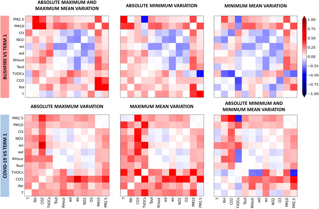
FIGURE 11. Significant inter-parameter correlation coefficient variation between Bushfire and Term 1 (upper row) and COVID-19 and Term 1 (lower row).

During COVID-19 lockdown, the correlations tended to get stronger as more stable conditions were established across the building. The absolute maximum difference (0.73) occurred in a non-conditioned, south-oriented staff office on Level 4 and affected the relationship between indoor CO₂ and wind speed. As people’s contribution to CO₂ emissions disappeared, the relative weight of outdoor carbon dioxide transported by the wind increased. The maximum mean difference (0,17) was recorded in a computer lab on level 3, where almost all correlations increased by more than 0.5. This suggests that occupancy dictates the IEQ level in spaces of standard high-density, on all counts. The absolute minimum difference (−0.42) was detected in the centrally located studio in the basement and affected the TVOCs-PM_2.5 relationship. This location experienced also the minimum mean difference (0.08), since the correlations across indoor parameters were strongly attenuated. This decrease in associativity is partly compensated by the increase in associativity with outdoor parameters, which, in the end, is the overarching effect of the lockdown.

Discussion and Design Guidelines

A public health imperative exists for educational buildings to be heat- and pollution-safe, particularly on account of escalating heatwaves and tropical nights events that impair night flush cooling (Gershunov et al., 2009; Dengel and Swainson, 2012). To achieve these objectives, results from fine-grained and long-term measurements can be used in identifying priority areas and emerging patterns, which can inform re-design strategies for IEQ preservation. These insights can be further useful for other buildings with similar building types, usage, and characteristics.

Focusing on room characteristics, we find that:

the absence of an air-conditioning system was conducive to greater heat stress, while its presence triggered higher average pollutant concentrations. This is particularly due to the fact that passive ventilation systems - such as louvres that are embedded to assist with air circulation in the building - entirely rely on manual interventions that are not commonly used. Accordingly, the optimum natural ventilation of the building envisioned in the design is hardly achieved. This results in significantly higher CO₂ levels in rooms with high occupancy, as users tend to be less sensitive to CO₂ levels, further supporting the need for automated demand-driven controls that can be actioned informed by real-time data;

north-exposure was associated with the hottest conditions, suggesting a non-efficient use of thermally massive materials, ineffectiveness of solar shading devices, and limited natural ventilation;

insufficient thermal insulation and air tightness result in excessively humid episodes in high-occupancy rooms close to the ground and facing south, where shading was most effective;

rooms located in the basement, which lack windows and mostly rely on air conditioning, experienced the best and worst heat stress conditions depending on manual interventions to condition the air and dissipate excess humidity.

Focusing on room use, we find that:

individual offices (mostly north-facing) exhibited most absolute maxima and minima, owing to the small air volume, the highly transmitting windowed side, and the extreme variability associated with occupancy patterns. These rooms also represent the highest user autonomy and, therefore, likelihood for implementing manual interventions. The use of portable A/C devices and the amount of electronic equipment should clearly be considered in individual offices to enhance heat index and IEQ levels;

computer labs exhibited the highest mean temperature, CO₂, and TVOCs, with significant extreme episodes. Being densely occupied, electronically closed, and prone to untimely comfort-restoring actions, these rooms, on average, act as sinks for heat and pollutants and fail at maintaining heat safe conditions. Particularly during extreme events such as bushfires, these rooms should be closely monitored and intensively ventilated to avoid unhealthy conditions for occupants. This further extend the service life of the electronic equipment from dust clogging;

studios exhibited HI conditions requiring caution and significant pollution episodes, with CO₂ crossing the unhealthy thresholds. These rooms were mostly located on lower floors, likely leading to the accumulation of pollutants from upper levels in addition to local emissions from typical equipment used on site. Relocation of studio-like environments with higher occupancy to upper floors should be considered;

multi-level study areas benefited from better air circulation, but were prone to extreme pollutant accumulation due to the presence of fully glazed facades that cannot be opened;

meeting rooms succeeded in maintaining the comfort zones on average, but exhibited very high-risk events during closed-door meetings. Both CO₂ and TVOCs could reach unhealthy levels in short periods of use. Due to concerns regarding noise levels, doors are often kept shut which leads to extremely unhealthy conditions particularly during extreme weather events. Large, acoustically-insulated grids or automated controls could be implemented to maintain adequate cross ventilation while addressing concerns regarding noise;

staff offices were typically heat-safe, thanks to extensive shading, very low occupancy, and AC provisions. Similar to individual offices, these spaces are also more likely to be subject to manual interventions. However, the presence of TVOC-emitting equipment and major renovations exacerbated TVOCs levels;

classrooms outperformed all other environments in terms of thermo-hygrometric conditions with no A/C in place, particularly due to their south exposure, the extensive provision of shadings and operable windows, and the efficient cross ventilation. The temperature typically lied in the 20–25°C range, the HI stayed within the heat-safe zone, and TVOCs never crossed the unhealthy threshold in warm periods. However, mean CO₂ levels could put sensitive people at risk and frequently crossed the unhealthy threshold, with further accumulation in wintertime when windows and doors were typically closed, thus stressing the need for year-round ventilation strategies;

Utility rooms (such as the print and media rooms) further exhibited unique characteristics. The print room reached CO₂ levels so high that health-threatening levels (even for short exposure) were the norm. Major redesign measures are imperative in order to meet minimum advised levels. On the other hand, the media room in the basement, which is sporadically used for media content production, frequently experienced extreme HI episodes due to unusually high humidity levels and equipment in use. This further suggests that utility rooms, even if not regularly occupied, require active control actions or redesign to avoid adverse IEQ conditions.

On top of this, the mutual information analysis revealed that 1) relative humidity is especially correlated with carbon dioxide levels, hence a better control over RH is expected to be extremely impactful on IAQ preservation; 2) during bushfire events, a major role is played by temperature and wind-related parameters, whereas during lockdown periods (i.e., in the absence of occupants) the influence of outdoor parameters becomes dominant; 3) elevation arbitrates the strength of correlation between thermo-hygrometric and air quality parameters. Future-proof re-design strategies should be built upon these associations.

Pertaining to the application of fine-grained IoT networks for assessing environmental quality, we note that in addition to insights gathered in this analysis, certain challenges and limitations should be considered. First, not only the spatial and temporal distribution of data collection but also the parameters monitored have a big impact on drawing insights from results. For instance, behavioural parameters - such as occupancy and manual interventions - are not commonly recorded in the environmental networks, but have a significant impact on IEQ particularly in educational buildings on university campuses. Here, room types are used as a proxy for determining occupancy patterns, but future measurement campaigns should consider collecting detailed behavioural data that focus the analyses solely on occupied hours. Similarly, detailed metadata on room characteristics are extremely hard to obtain and rarely incorporated in the IoT environmental data platforms. Here, exhaustive and manual surveys of rooms were conducted to determine room characteristics in the studied research (summarized in Supplementary Appendix Table A1). Future research should focus on automated integration of fine-grained building information with real-time sensor data, establishing a digital twin of buildings to effectively integrate, communicate, and analyze environmental quality. More importantly, such integration with building data can inform automated control actions that enhance IEQ. Lastly, larger deployment of sensors often dictates that sensors are lower cost which can have an impact on sensor accuracy and lifetime. Quality controls are applied in these analyses (before sensor installation and after data collection), but longer-term data collection likely requires recalibrations to account for sensor drifts and faulty devices. This is in addition to maintenance challenges regarding theft and vandalism that have been experienced in this project.

On a conclusive note, the proposed monitoring design departs from conventional data collection methods, relying on controlled-environment testing or short-term monitoring. It captures the IEQ nuances in a realistic and unbiased fashion. Accordingly, we did not intend, nor had the ability, to control for environmental/occupancy conditions that the building was going to be subject to in the long term. This non-invasive approach makes it harder to disclose clear patterns and run comparative assessments, yet it gives us the chance to appreciate the complexity of a living environment without data degradation or alteration.

Conclusion

In this study, we targeted an educational building in Sydney, whose proclivity to IEQ deterioration is aggravated by design inefficiencies and local weather extremes. A novel, low-cost, multi-parameter IOT sensor network was deployed to fully depict the spatial heterogeneity and temporal variability in terms of thermal comfort and air quality. The data has been analysed through a variety of statistical methods including unconditioned and conditioned mutual information analysis and through established comfort metrics on account of room characteristics, room use, season, weather extremes and standard versus atypical occupancy patterns as those recorded during the bushfire season and the COVID-19 pandemic. By merging the results presented in Results section, a variety of redesign strategies could be delineated (Discussion and Design Guidelines section) thanks to the fine-grained, site-specific monitoring of each room type across different floors and orientations. Such a detailed analysis compensates for less perceivable threats, pinpoints passive ventilation inefficiencies, identifies the room for improvement, and suggests an urgent need to prioritize building air tightness improvement, appropriate filtration techniques and smart logics. This study offers a roadmap for other campaigns alike in order to verify climate dependencies and general patterns and move towards more resilient and healthy educational buildings. However, future directions in IoT environmental sensor networks should focus on not only covering spatial heterogeneity of IEQ, but also consider comprehensive data collection (encompassing environmental and behavioural factors), integration of building metadata, and dynamic quality controls to provide most comprehensive insights.

Data Availability Statement

The raw data supporting the conclusion of this article will be made available by the authors, without undue reservation.

Author Contributions

NN and CP conceived the presented idea, established and maintained the IoT sensor network, and supervised the project. FZ obtained the data and performed quality controls. GU analysed the data and wrote the manuscript with support from NN, CP, and FZ.

Conflict of Interest

The authors declare that the research was conducted in the absence of any commercial or financial relationships that could be construed as a potential conflict of interest.

Publisher’s Note

All claims expressed in this article are solely those of the authors and do not necessarily represent those of their affiliated organizations, or those of the publisher, the editors and the reviewers. Any product that may be evaluated in this article, or claim that may be made by its manufacturer, is not guaranteed or endorsed by the publisher.

Supplementary Material

The Supplementary Material for this article can be found online at: https://www.frontiersin.org/articles/10.3389/fenvs.2021.725974/full#supplementary-material

References

Abcb (2018). Indoor Air Quality Handbook. CANBERRA ACT.

Google Scholar

Abdul Rahman, I., Putra, J. C. P., and Nagapan, S. (2014). Correlation of Indoor Air Quality with Working Performance in Office Building. Mod. Appl. Sci. 8, 153–160. doi:10.5539/mas.v8n6p153

CrossRef Full Text | Google Scholar

Alfano, F. R. A., Palella, B. I., and Riccio, G. (2011). Thermal Environment Assessment Reliability Using Temperature -Humidity Indices. Ind. Health 49, 95–106. doi:10.2486/indhealth.ms1097

PubMed Abstract | CrossRef Full Text | Google Scholar

Almeida, R. M. S. F., and de Freitas, V. P. (2014). Indoor Environmental Quality of Classrooms in Southern European Climate. Energy and Buildings 81, 127–140. doi:10.1016/j.enbuild.2014.06.020

CrossRef Full Text | Google Scholar

Alonso, A., Llanos, J., Escandón, R., and Sendra, J. J. (2021). Effects of the COVID-19 Pandemic on Indoor Air Quality and Thermal Comfort of Primary Schools in Winter in a Mediterranean Climate. Sustainability 13, 2699. doi:10.3390/su13052699

CrossRef Full Text | Google Scholar

Andualem, Z., Gizaw, Z., Bogale, L., and Dagne, H. (2019). Indoor Bacterial Load and its Correlation to Physical Indoor Air Quality Parameters in Public Primary Schools. Multidiscip. Respir. Med. 14, 2. doi:10.1186/s40248-018-0167-y

PubMed Abstract | CrossRef Full Text | Google Scholar

Annesi-Maesano, I., Baiz, N., Banerjee, S., Rudnai, P., and Rive, S.The SINPHONIE Group (2013). Indoor Air Quality and Sources in Schools and Related Health Effects. J. Toxicol. Environ. Health B 16, 491–550. doi:10.1080/10937404.2013.853609

CrossRef Full Text | Google Scholar

ANSI/ASHRAE (2016). ANSI/ASHRAE 62-1 Ventilation for Acceptable Indoor Air Quality.

Google Scholar

Apte, M. G., and Erdmann, C. A. (2002). Associations of Indoor Carbon Dioxide Concentrations, VOCS, Environmental Susceptibilities with Mucous Membrane and Lower Respiratory Sick Building Syndrome Symptoms in the BASE Study: Analyses of the 100 Building Dataset. Berkeley, CA: Lawrence Berkeley National Lab. doi:10.2172/806126

CrossRef Full Text | Google Scholar

Apte, M. G., Fisk, W. J., and Daisey, J. M. (2000). Associations between Indoor CO2 Concentrations and Sick Building Syndrome Symptoms in U.S. Office Buildings: an Analysis of the 1994-1996 BASE Study Data. Indoor Air 10, 246–257. doi:10.1034/j.1600-0668.2000.010004246.x

PubMed Abstract | CrossRef Full Text | Google Scholar

Australian Government (2020). Air Quality – Indoor Air. Department of Agriculture, Water and the Environment. Available at: https://www.environment.gov.au/protection/air-quality/indoor-air (Accessed October 3, 2021).

Google Scholar

Baird, G., and Marriage, G. (2015). User Satisfaction with Academic Buildings-Ffindings from post Occupancy Evaluations. Available at: http://anzasca.net/wp-content/uploads/2015/12/059_Baird_Marriage_ASA2015.pdf.

Google Scholar

Baird, G. (2013). Sustainable Buildings–Best and Worst Performers in Terms of Comfort, Health and Productivity. Smart and Sustainable Built Environments. Available at: https://www.researchgate.net/profile/Nurul_Sakina_Mokhtar_Azizi2/publication/283479398_Proceedings_of_Smart_and_Sustainable_Built_Environments/links/5639c01108aecf1d92a9fa63/Proceedings-of-Smart-and-Sustainable-Built-Environments.pdf#page=365.

Google Scholar

Baird, G. (2003). The Architectural Expression of Environmental Control Systems. Taylor & Francis. doi:10.4324/9780203362488

CrossRef Full Text

Bolan, N. (2020). A Burning Issue: Volatile Organic Compounds from Bushfire. Chem. Aust., 21–23.

Google Scholar

BOM (2021a). Australian Government Climate Classification Maps. Available at: http://www.bom.gov.au/jsp/ncc/climate_averages/climate-classifications/index.jsp?maptype=kpn#maps (Accessed April 29, 2021).

Google Scholar

BOM (2021). Climate Statistics for Australian Locations - Summary Statistics SYDNEY. Available at: http://www.bom.gov.au/climate/averages/tables/cw_066062.shtml (Accessed March 23, 2021).

Google Scholar

Calderón-Garcidueñas, L., Calderón-Garcidueñas, A., Torres-Jardón, R., Avila-Ramírez, J., Kulesza, R. J., and Angiulli, A. D. (2015). Air Pollution and Your Brain: what Do You Need to Know Right Now. Prim. Health Care Res. Dev. 16, 329–345. doi:10.1017/s146342361400036x

PubMed Abstract | CrossRef Full Text | Google Scholar

Cellucci, C. J., Albano, A. M., and Rapp, P. E. (2005). Statistical Validation of Mutual Information Calculations: Comparison of Alternative Numerical Algorithms. Phys. Rev. E Stat. Nonlin. Soft Matter Phys. 71, 066208. doi:10.1103/PhysRevE.71.066208

PubMed Abstract | CrossRef Full Text | Google Scholar

Chatzidiakou, L., Mumovic, D., and Summerfield, A. J. (2012). What Do We Know about Indoor Air Quality in School Classrooms? A Critical Review of the Literature. Intell. Buildings Int. 4, 228–259. doi:10.1080/17508975.2012.725530

CrossRef Full Text | Google Scholar

Chernev, L., Targino, A. C., Coraiola, G. C., and Krecl, P. (2012). “Outdoor thermal comfort Indices and Their Relation to Land Use over an Urban Area during winter Time,” in XI Congresso Argentino de Meteorologia (Mendoza, Argentina. Available at: http://www.congremet.prmarg.org/upload/chernevlucas.pdf.

Google Scholar

Daisey, J. M., Angell, W. J., and Apte, M. G. (2003). Indoor Air Quality, Ventilation and Health Symptoms in Schools: an Analysis of Existing Information. Indoor Air 13, 53–64. doi:10.1034/j.1600-0668.2003.00153.x

PubMed Abstract | CrossRef Full Text | Google Scholar

Dengel, A., and Swainson, M. (2012). Overheating in New Homes: A Review of the Evidence. Milton Keynes: Building Research Establishment.

Google Scholar

Dorizas, P. V., Assimakopoulos, M.-N., and Santamouris, M. (2015). A Holistic Approach for the Assessment of the Indoor Environmental Quality, Student Productivity, and Energy Consumption in Primary Schools. Environ. Monit. Assess. 187, 259. doi:10.1007/s10661-015-4503-9

PubMed Abstract | CrossRef Full Text | Google Scholar

Ebenstein, A., Lavy, V., and Roth, S. (2016). The Long-Run Economic Consequences of High-Stakes Examinations: Evidence from Transitory Variation in Pollution. Am. Econ. J. Appl. Econ. 8, 36–65. doi:10.1257/app.20150213

CrossRef Full Text | Google Scholar

Eide, E. R., Showalter, M. H., and Goldhaber, D. D. (2010). The Relation between Children's Health and Academic Achievement. Child. Youth Serv. Rev. 32, 231–238. doi:10.1016/j.childyouth.2009.08.019

CrossRef Full Text | Google Scholar

Evrard, A.-S., Hmon, D., Billon, S., Laurier, D., Jougla, E., Tirmarche, M., et al. (2006). Childhood Leukemia Incidence and Exposure to Indoor Radon, Terrestrial and Cosmic Gamma Radiation. Health Phys. 90, 569–579. doi:10.1097/01.hp.0000198787.93305.35

PubMed Abstract | CrossRef Full Text | Google Scholar

Fang, L., Clausen, G., and Fanger, P. O. (1998). Impact of Temperature and Humidity on the Perception of Indoor Air Quality. Indoor Air 8, 80–90. doi:10.1111/j.1600-0668.1998.t01-2-00003.x

CrossRef Full Text | Google Scholar

Fraser, A. M., and Swinney, H. L. (1986). Independent Coordinates for Strange Attractors from Mutual Information. Phys. Rev. A. 33, 1134–1140. doi:10.1103/physreva.33.1134

PubMed Abstract | CrossRef Full Text | Google Scholar

Frenzel, S., and Pompe, B. (2007). Partial Mutual Information for Coupling Analysis of Multivariate Time Series. Phys. Rev. Lett. 99, 204101. doi:10.1103/physrevlett.99.204101

PubMed Abstract | CrossRef Full Text | Google Scholar

Gallego, E., Roca, F. J., Perales, J. F., and Guardino, X. (2011). “Assessment of Chemical Hazards in Sick Building Syndrome Situations: Determination of Concentrations and Origin of VOCs in Indoor Air Environments by Dynamic Sampling and TD-GC/MS Analysis,” in Sick Building Syndrome in Public Buildings and Workplaces (Springer), 289–333. doi:10.1007/978-3-642-17919-8_16

CrossRef Full Text | Google Scholar

Gent, J. F., Triche, E. W., Holford, T. R., Belanger, K., Bracken, M. B., Beckett, W. S., et al. (2003). Association of Low-Level Ozone and fine Particles with Respiratory Symptoms in Children with Asthma. JAMA 290, 1859–1867. doi:10.1001/jama.290.14.1859

PubMed Abstract | CrossRef Full Text | Google Scholar

Gershunov, A., Cayan, D. R., and Iacobellis, S. F. (2009). The Great 2006 Heat Wave over California and Nevada: Signal of an Increasing Trend. J. Clim. 22, 6181–6203. doi:10.1175/2009jcli2465.1

CrossRef Full Text | Google Scholar

Government of Canada (2021). Wind Chill and Humidex Calculators. Available at: https://weather.gc.ca/windchill/wind_chill_e.html (Accessed March 24, 2021).

Google Scholar

Haddad, S., Synnefa, A., Ángel Padilla Marcos, M., Paolini, R., Delrue, S., Prasad, D., et al. (2021). On the Potential of Demand-Controlled Ventilation System to Enhance Indoor Air Quality and thermal Condition in Australian School Classrooms. Energy and Buildings 238, 110838. doi:10.1016/j.enbuild.2021.110838

CrossRef Full Text | Google Scholar

Havenith, G. (2007). Metabolic Rate and Clothing Insulation Data of Children and Adolescents during Various School Activities. Ergonomics 50, 1689–1701. doi:10.1080/00140130701587574

PubMed Abstract | CrossRef Full Text | Google Scholar

Haverinen-Shaughnessy, U., Shaughnessy, R. J., Cole, E. C., Toyinbo, O., and Moschandreas, D. J. (2015). An Assessment of Indoor Environmental Quality in Schools and its Association with Health and Performance. Building Environ. 93, 35–40. doi:10.1016/j.buildenv.2015.03.006

CrossRef Full Text | Google Scholar

Humphreys, M. A., Rijal, H. B., and Nicol, J. F. (2013). Updating the Adaptive Relation between Climate and comfort Indoors; New Insights and an Extended Database. Building Environ. 63, 40–55. doi:10.1016/j.buildenv.2013.01.024

CrossRef Full Text | Google Scholar

IPCC Fifth Assessment Report (AR5) (2013). WMO, IPCC Secretariat.

Google Scholar

Kim, E.-K., Kim, G.-S., and Park, J.-S. (2009). Comparison of Activity Factor, Predicted Resting Metabolic Rate, and Intakes of Energy and Nutrients between Athletic and Non-athletic High School Students. J. Korean Diet. Assoc. 15, 52–68.

Google Scholar

Klepeis, N. E., Nelson, W. C., Ott, W. R., Robinson, J. P., Tsang, A. M., Switzer, P., et al. (2001). The National Human Activity Pattern Survey (NHAPS): a Resource for Assessing Exposure to Environmental Pollutants. J. Expo. Sci. Environ. Epidemiol. 11, 231–252. doi:10.1038/sj.jea.7500165

PubMed Abstract | CrossRef Full Text | Google Scholar

Laarne, P., Zaidan, M. A., and Nieminen, T. (2021). Ennemi: Non-linear Correlation Detection with Mutual Information. SoftwareX 14, 100686. doi:10.1016/j.softx.2021.100686

CrossRef Full Text | Google Scholar

Lacetera, N., Bernabucci, U., Khalifa, H. H., Ronchi, B., and Nardone, A. (2003). Interaction between Climate and Animal Production. Wageningen Academic Publishers.

Google Scholar

Lazović, I., Stevanović, Ž. M., Jovašević-Stojanović, M., Živković, M. M., and Banjac, M. J. (2016). Impact of CO2 Concentration on Indoor Air Quality and Correlation with Relative Humidity and Indoor Air Temperature in School Buildings in Serbia. Therm. Sci. 20, S297–S307. doi:10.2298/tsci150831173l

CrossRef Full Text | Google Scholar

Chen, L., Jennison, B. L., Yang, W., and Omaye, S. T. (2000). Elementary School Absenteeism and Air Pollution. Inhalation Toxicol. 12, 997–1016. doi:10.1080/08958370050164626

CrossRef Full Text | Google Scholar

Li, C., Wang, W., Xiong, J., and Chen, P. (2014). Sensitivity Analysis for Urban Drainage Modeling Using Mutual Information. Entropy 16, 5738–5752. doi:10.3390/e16115738

CrossRef Full Text | Google Scholar

Livada, I., Synnefa, A., Haddad, S., Paolini, R., Garshasbi, S., Ulpiani, G., et al. (2019). Time Series Analysis of Ambient Air-Temperature during the Period 1970-2016 over Sydney, Australia. Sci. Total Environ. 648, 1627–1638. doi:10.1016/j.scitotenv.2018.08.144

PubMed Abstract | CrossRef Full Text | Google Scholar

Loh, J. Y. S., and Andamon, M. M. A Review of IAQ Standards and Guidelines for Australian and New Zealand School Classrooms. anzasca.Net. Available at: http://anzasca.net/wp-content/uploads/2017/11/ASA_2017_Loh_Andamon.pdf.

Google Scholar

Luo, M., Hong, Y., and Pantelic, J. (2021). Determining Building Natural Ventilation Potential via IoT-Based Air Quality Sensors. Front. Environ. Sci. 9. doi:10.3389/fenvs.2021.634570

CrossRef Full Text | Google Scholar

Meiss, A., Jimeno-Merino, H., and Poza-Casado, I. (2021). Indoor Air Quality in Naturally Ventilated Classrooms. Lessons Learned from a Case Study in a COVID-19 Scenario. Sustain. Sci. Pract. Pol. 13 (15), 8446. doi:10.3390/su13158446

CrossRef Full Text | Google Scholar

Mendell, M. J., Eliseeva, E. A., Davies, M. M., Spears, M., Lobscheid, A., Fisk, W. J., et al. (2013). Association of Classroom Ventilation with Reduced Illness Absence: a Prospective Study in California Elementary Schools. Indoor Air 23, 515–528. doi:10.1111/ina.12042

PubMed Abstract | CrossRef Full Text | Google Scholar

Mi, Y.-H., Norbäck, D., Tao, J., Mi, Y.-L., and Ferm, M. (2006). Current Asthma and Respiratory Symptoms Among Pupils in Shanghai, China: Influence of Building Ventilation, Nitrogen Dioxide, Ozone, and Formaldehyde in Classrooms. Indoor Air 16, 454–464. doi:10.1111/j.1600-0668.2006.00439.x

PubMed Abstract | CrossRef Full Text | Google Scholar

Moran, D. S., Shapiro, Y., Epstein, Y., Matthew, W., and Pandolf, K. B. (1998). “A Modified Discomfort index (MDI) as an Alternative to the Wet Bulb globe Temperature (WBGT),” in Environmental Ergonomics VIII. Editors J. A. Hodgdon, J. H. Heaney, and M. J. Buono, 77–80.

Google Scholar

Mumtaz, R., Zaidi, S. M. H., Shakir, M. Z., Shafi, U., Malik, M. M., Haque, A., et al. (2021). Internet of Things (IoT) Based Indoor Air Quality Sensing and Predictive Analytic-A COVID-19 Perspective. Electronics 10, 184. doi:10.3390/electronics10020184

CrossRef Full Text | Google Scholar

Nazarian, N., and Lee, J. K. (2021). Personal Assessment of Urban Heat Exposure: a Systematic Review. Environ. Res. Lett. 16, 033005. doi:10.1088/1748-9326/abd350

CrossRef Full Text | Google Scholar

NOAA (2021). Summer Weather Safety and Survival: the Heat Index. Available at: https://www.weather.gov/oun/safety-summer-heatindex (Accessed March 24, 2021).

Google Scholar

Norbäck, D., and Nordström, K. (2008). Sick Building Syndrome in Relation to Air Exchange Rate, CO2, Room Temperature and Relative Air Humidity in university Computer Classrooms: an Experimental Study. Int. Arch. Occup. Environ. Health 82, 21–30. doi:10.1007/s00420-008-0301-9

PubMed Abstract | CrossRef Full Text | Google Scholar

Nws, U. (2021). What Is the Heat index. Available at: https://www.weather.gov/ama/heatindex (Accessed March 24, 2021).

Google Scholar

Ortiz Perez, A., Bierer, B., Scholz, L., Wöllenstein, J., and Palzer, S. (2018). A Wireless Gas Sensor Network to Monitor Indoor Environmental Quality in Schools. Sensors 18, 4345. doi:10.3390/s18124345

CrossRef Full Text | Google Scholar

Palacios Temprano, J., Eichholtz, P., Willeboordse, M., and Kok, N. (2020). Indoor Environmental Quality and Learning Outcomes: Protocol on Large-Scale Sensor Deployment in Schools. BMJ Open 10, e031233. doi:10.1136/bmjopen-2019-031233

CrossRef Full Text | Google Scholar

Potchter, O., Cohen, P., Lin, T.-P., and Matzarakis, A. (2018). Outdoor Human thermal Perception in Various Climates: A Comprehensive Review of Approaches, Methods and Quantification. Sci. Total Environ. 631-632, 390–406. doi:10.1016/j.scitotenv.2018.02.276

PubMed Abstract | CrossRef Full Text | Google Scholar

Quinn, A., Tamerius, J. D., Perzanowski, M., Jacobson, J. S., Goldstein, I., Acosta, L., et al. (2014). Predicting Indoor Heat Exposure Risk during Extreme Heat Events. Sci. Total Environ. 490, 686–693. doi:10.1016/j.scitotenv.2014.05.039

PubMed Abstract | CrossRef Full Text | Google Scholar

Rajagopalan, P., and Goodman, N. (2021). Improving the Indoor Air Quality of Residential Buildings during Bushfire Smoke Events. Climate 9, 32. doi:10.3390/cli9020032

CrossRef Full Text | Google Scholar

Reid, C. E., Considine, E. M., Watson, G. L., Telesca, D., Pfister, G. G., and Jerrett, M. (2019). Associations between Respiratory Health and Ozone and fine Particulate Matter during a Wildfire Event. Environ. Int. 129, 291–298. doi:10.1016/j.envint.2019.04.033

PubMed Abstract | CrossRef Full Text | Google Scholar

Rocca, M., Leccese, F., and Salvadori, G. (2020). “Health and Well-Being in Indoor Work Environments: Features of an Expert Assessment Campaign in an Italian University Hospital,” in 2020 IEEE International Conference on Environment and Electrical Engineering and 2020 IEEE Industrial and Commercial Power Systems Europe (EEEIC/I CPS Europe), Madrid, Spain, 9-12 June 2020 (IEEE), 1–6. doi:10.1109/eeeic/icpseurope49358.2020.9160493

CrossRef Full Text | Google Scholar

Rothfusz, L. P., and Headquarters, N. S. R. (1990). The Heat index Equation (Or, More than You Ever Wanted to Know about Heat index). Fort Worth, Texas: National Oceanic and Atmospheric Administration, National Weather Service, Office of Meteorology, 9023. Available at: http://wonder.cdc.gov/wonder/help/Climate/ta_htindx.PDF.

Google Scholar

Ryu, U., Wang, J., Kim, T., Kwak, S., and UJuhyok, J. (2018). Construction of Traffic State Vector Using Mutual Information for Short-Term Traffic Flow Prediction. Transportation Res. C: Emerging Tech. 96, 55–71. doi:10.1016/j.trc.2018.09.015

CrossRef Full Text | Google Scholar

Saad, S. M., Shakaff, A. Y. M., Saad, A. R. M., Yusof, A. M., Andrew, A. M., Zakaria, A., et al. (2017). Development of Indoor Environmental index: Air Quality index and thermal comfort index. AIP Conf. Proc. 1808, 020043. doi:10.1063/1.4975276

CrossRef Full Text | Google Scholar

Saggu, G. S., Mittal, S. K., Agarwal, R., and Beig, G. (2018). Epidemiological Study on Respiratory Health of School Children of Rural Sites of Malwa Region (India) during Post-harvest Stubble Burning Events. MAPAN 33, 281–295. doi:10.1007/s12647-018-0259-3

CrossRef Full Text | Google Scholar

Santamouris, M., Haddad, S., Fiorito, F., Osmond, P., Ding, L., Prasad, D., et al. (2017). Urban Heat Island and Overheating Characteristics in Sydney, Australia. An Analysis of Multiyear Measurements. Sustainability 9, 712. doi:10.3390/su9050712

CrossRef Full Text | Google Scholar

Santamouris, M. (2020). Recent Progress on Urban Overheating and Heat Island Research. Integrated Assessment of the Energy, Environmental, Vulnerability and Health Impact. Synergies with the Global Climate Change. Energy and Buildings 207, 109482. doi:10.1016/j.enbuild.2019.109482

CrossRef Full Text | Google Scholar

Satish, U., Mendell, M. J., Shekhar, K., Hotchi, T., Sullivan, D., Streufert, S., et al. (2012). Is CO2an Indoor Pollutant? Direct Effects of Low-To-Moderate CO2Concentrations on Human Decision-Making Performance. Environ. Health Perspect. 120, 1671–1677. doi:10.1289/ehp.1104789

PubMed Abstract | CrossRef Full Text | Google Scholar

Schibuola, L., and Tambani, C. (2020). Indoor Environmental Quality Classification of School Environments by Monitoring PM and CO2 Concentration Levels. Atmos. Pollut. Res. 11, 332–342. doi:10.1016/j.apr.2019.11.006

CrossRef Full Text | Google Scholar

Simons, E., Hwang, S.-A., Fitzgerald, E. F., Kielb, C., and Lin, S. (2010). The Impact of School Building Conditions on Student Absenteeism in Upstate New York. Am. J. Public Health 100, 1679–1686. doi:10.2105/ajph.2009.165324

CrossRef Full Text | Google Scholar

Stazi, F., Naspi, F., Ulpiani, G., and Di Perna, C. (2017). Indoor Air Quality and thermal comfort Optimization in Classrooms Developing an Automatic System for Windows Opening and Closing. Energy and Buildings 139, 732–746. doi:10.1016/j.enbuild.2017.01.017

CrossRef Full Text | Google Scholar

Taylor, L., Watkins, S. L., Marshall, H., Dascombe, B. J., and Foster, J. (2015). The Impact of Different Environmental Conditions on Cognitive Function: A Focused Review. Front. Physiol. 6, 372. doi:10.3389/fphys.2015.00372

PubMed Abstract | CrossRef Full Text | Google Scholar

Ulpiani, G., Ranzi, G., and Santamouris, M. (2020). Experimental Evidence of the Multiple Microclimatic Impacts of Bushfires in Affected Urban Areas: The Case of Sydney during the 2019/2020 Australian Season. Environ. Res. 2, 065005. doi:10.1088/2515-7620/ab9e1a

CrossRef Full Text | Google Scholar

Ulpiani, G., Ranzi, G., and Santamouris, M. (2021). Local Synergies and Antagonisms between Meteorological Factors and Air Pollution: A 15-year Comprehensive Study in the Sydney Region. Sci. Total Environ. 788, 147783. doi:10.1016/j.scitotenv.2021.147783

PubMed Abstract | CrossRef Full Text | Google Scholar

Umweltbundesamt (2007). Evaluation of Indoor Air Contaminants by Means of Reference and Guideline Values. Bundesgesundheitsblatt Gesundheitsforschung Gesundheitsschutz 50, 990–1005. doi:10.1007/s00103-007-0290-y

PubMed Abstract | CrossRef Full Text | Google Scholar

UNSW (2021). Myair Air Quality Sensors. City Futures Research Centre. Available at: https://citydata.be.unsw.edu.au/layers/geonode%3Amyair#more (Accessed March 23, 2021).

Google Scholar

World Health Organization (2000). Air Quality Guidelines for Europe. Copenhagen: WHO Reg Publ Eur Ser, V–273.

Google Scholar

Wyon, D. P. (2004). The Effects of Indoor Air Quality on Performance and Productivity. Indoor Air 14 (7), 92–101. doi:10.1111/j.1600-0668.2004.00278.x

CrossRef Full Text | Google Scholar

Yun, G. Y., Ngarambe, J., Duhirwe, P. N., Ulpiani, G., Paolini, R., Haddad, S., et al. (2020). Predicting the Magnitude and the Characteristics of the Urban Heat Island in Coastal Cities in the Proximity of Desert Landforms. The Case of Sydney. Sci. Total Environ. 709, 136068. doi:10.1016/j.scitotenv.2019.136068

PubMed Abstract | CrossRef Full Text | Google Scholar

Zaidan, M. A., Dada, L., Alghamdi, M. A., Al-Jeelani, H., Lihavainen, H., Hyvärinen, A., et al. (2019). Mutual Information Input Selector and Probabilistic Machine Learning Utilisation for Air Pollution Proxies. Appl. Sci. 9, 4475. doi:10.3390/app9204475

CrossRef Full Text | Google Scholar

Zaidan, M. A., Haapasilta, V., Relan, R., Paasonen, P., Kerminen, V.-M., Junninen, H., et al. (2018). Exploring Non-linear Associations between Atmospheric New-Particle Formation and Ambient Variables: a Mutual Information Approach. Atmos. Chem. Phys. 18, 12699–12714. doi:10.5194/acp-18-12699-2018

CrossRef Full Text | Google Scholar

Zhao, D., Azimi, P., and Stephens, B. (2015). Evaluating the Long-Term Health and Economic Impacts of Central Residential Air Filtration for Reducing Premature Mortality Associated with Indoor Fine Particulate Matter (PM2.5) of Outdoor Origin. Ijerph 12, 8448–8479. doi:10.3390/ijerph120708448

PubMed Abstract | CrossRef Full Text | Google Scholar