A New Global Ocean Climatology

A new global ocean temperature and salinity climatology is proposed for two time periods: a long time mean using multiple sensor data for the 1900–2017 period and a shorter time mean using only profiling float data for the 2003–2017 period. We use the historical database of World Ocean Database 2018. The estimation approach is novel as an additional quality control procedure is implemented, along with a new mapping algorithm based on Data Interpolating Variational Analysis. The new procedure, in addition to the traditional quality control approach, resulted in low sensitivity in terms of the first guess field choice. The roughness index and the root mean square of residuals are new indices applied to the selection of the free mapping parameters along with sensitivity experiments. Overall, the new estimates were consistent with previous climatologies, but several differences were found. The cause of these discrepancies is difficult to identify due to several differences in the procedures. To minimise these uncertainties, a multi-model ensemble mean is proposed as the least uncertain estimate of the global ocean temperature and salinity climatology.

1 Introduction

Defining the climatological state of the ocean is a formidable task. Climatology can be defined as the study of the statistics of environmental variables that characterise the ocean’s physical and biochemical state. The focus of this work is on estimating the monthly mean values of temperature and salinity in the global ocean using data derived from historical observational records. Climatology is an essential input to numerical ocean models in terms of initialization and validation, and is intrinsically useful for understanding climate anomalies.

Standardising historical observations is a major challenge in climatological studies, in terms of metadata and quality control. The observations are collected from numerous sources and contain various errors. Thus, a robust quality control procedure is essential before any kind of analysis is conducted. Interpolating or mapping the observations is also major step in estimating climatologies. As defined by Daley (1993): “Spatial analysis is the estimation by numerical algorithm of state variables on a three-dimensional regular grid from observations available at irregularly distributed locations.” These numerical algorithms are based on theoretical and statistical assumptions that have significantly evolved over the past 20 years. Such techniques are referred as interpolation schemes.

Our analysis is based upon the World Ocean Data (WOD) archive of temperature and salinity profiles, which is probably the most comprehensive archive of data collected in the 20th century. The database already contains quality flagged profiles, which are described later in the paper. We applied another layer of quality checks to this, which were found to be significant as they eliminate further outliers.

The first global ocean gridded climatology, referred to as the World Ocean Atlas (WOA), was proposed by Levitus (1982) and is the basis for all subsequent estimates. The WOA has been regularly updated every 4 years since 1994. WOA uses the basic interpolation schemes defined by Barnes (1964). We use the latest WOD18 and WOA18 updates (Garcia et al., 2018), and (Locarnini et al., 2019; Zweng et al., 2019). The WOCE (World Ocean Circulation Experiment) Argo Hydrographic Global Ocean Climatology [WAGHC, Gouretski (2019)] is another global ocean climatological estimate and is the first to be produced at isopycnal and isobaric levels. The WAGHC interpolation scheme is based on Objective Analysis (OA) following Gandin (1960). In this study, we propose a new climatology developed within the framework of the SeaDataCloud project (Simoncelli et al., 2021) and computed with the Data Interpolating Variational Analysis [DIVAnd, (Brasseur, 1991), Troupin et al. (2012), and Barth et al. (2014)]. The SeaDataCloud global climatology is available from the SeaDataNet web catalog ¹ together with its relative Product Information Document (Shahzadi et al., 2020), (Shahzadi et al., 2020). Hereafter, it will be referred as SDC climatology, and a climatology using the Objective Analysis (OA) interpolation scheme of Bretherton et al. (1976), for the first time adapted to the global ocean by Jia et al. (2016), referred to as B-OA (Bretherton et al., 1976).

An obvious question is why another climatology is required. Climatologies are based on different observational datasets and use different interpolation schemes, so they address uncertainties in different ways. The specific interpolation of observations across land-sea boundaries represents a common uncertainty. Most established interpolating algorithms do not naturally consider objective methods that prohibit the use of observations across land-sea boundaries, which is an important characteristics of our algorithm. To show deviations between climatological interpolating algorithms at the land-ocean interface, we analyzed the differences among climatologies around peninsulas. For example, in the Isthmus of Panama, a narrow land area between the Caribbean Sea and the Pacific Ocean, observations could be misinterpreted, as they span unconnected ocean water masses. Figure 1 gives a comparison of the four available climatologies, and it is clear that they give very different estimates. In Figure 1C the B-OA shows that salinity spreads from the Pacific to the Atlantic along the Columbian coast. By contrast, Figure 1D demonstrates that the SDC climatology completely suppresses the contamination of the Caribbean Sea with Pacific Ocean salinities and vice-versa. However, in WAGHC and WOA, despite the use of the separate first guess fields across the Isthmus (Tim Boyer personal communications, and an anonymous reviewer), low salinity anomalies are reported for the Caribbean Sea, which are not present in the other gridded products. As the interpolation scheme and first guess field are computed separately in each basin in these two estimates then salinity variations among these estimates could be due to different observations used or the interpolation scheme. Another difference between climatologies is evident along the Louisiana coasts of the Gulf of Mexico, where the Mississippi river outflow dominates, which could be due to the algorithm, the first guess or the volume of data used in the analyses. Climatologies may therefore differ both qualitatively and quantitatively in general and specific aspects. DIVAnd objectively solves the problem of the interpolation of oceanographic observations across land boundaries, but it is similar to other statistical models as it makes assumptions about the statistical distribution parameters of the ocean variables of interest. Thus, a multi-model ensemble of all available climatologies is likely to provide a more accurate solution, as demonstrated later in this paper.

FIGURE 1

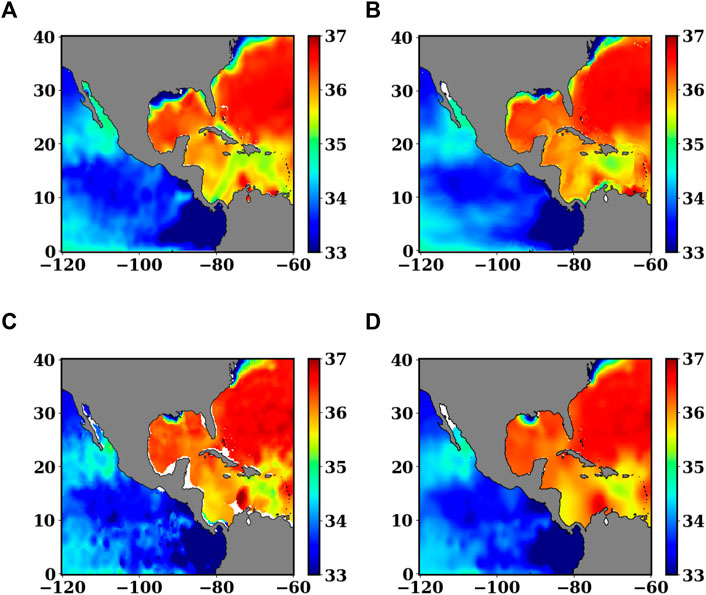
FIGURE 1. January salinity near the Panama Isthmus. (A) WOA18 estimate (correlation length = 214 km, using all data from WOD18), (B) WAGHC (correlation length = 333 km, signal to noise ratio = 0.5, using data from WOD13, in particular Ocean Station Data, Conductivity Depth Temperature, Profiling Floats and Autonomous Pinniped, with additional data from the Alfred Wegener Institute, Bremerhaven, and from other institutions in Canada), (C) B-OA estimate (correlation length = 300 km and observational error variance = 0.3), and (D) DIVAnd estimate (correlation length = 300 km and noise to signal ratio equal to 0.5).

The main objective of this study is to estimate a global ocean climatology using DIVAnd, after applying proper quality control to the historical dataset. The additional quality control algorithm we use is defined in section 2.1. Sensitivity experiments are also conducted for interpolation parameters such as the signal to noise ratio and the field correlation length. Finally, the results are compared with the WOA18 and WAGHC datasets. Those for the B-OA are disregarded because they are similar to the results for the WAGHC.

In section 2, the historical datasets used for climatology are reviewed together with the quality control procedure. The interpolation scheme and the implementation domain, together with the choices of the interpolation parameters, are discussed in section 3. Monthly mean temperature and salinity fields are compared with those of other climatologies in the section 4 while the section 5 concludes the paper.

2 Historical Datasets

Two climatology versions were estimated based on two datasets extracted from the World Ocean Database 18 [WOD18, Garcia et al. (2018)]. Dataset1 (see Table 1) uses multiple platforms, such as bottle data from Ocean Station Data (OSD) and Conductivity Temperature and Depth (CTD) from ship surveys, Mooring Buoys (MRBs) and Profiling Floats (PFLs). MRB profiles are only distributed across the equatorial and tropical regions, while CTD, OSD and PFL profiles cover the global ocean domain. The data from other available platforms were not used because we considered corresponding measurements of temperature and salinity and an approximately equal number of profiles for the surface and the upper pycnocline. Thus, Expendable Bathythermograph (XBT) and Mechanical Bathythermograph (MBT) data were disregarded because only temperature measurements were available. Drifting Buoy (DRB), and Surface-Only (SUR) data were also not selected because the recordings for these are only taken at the surface, and Autonomous Pinniped Bathythermograph (APB) and gliders (GLD) were not used because they consist of high temporal resolution measurements that are not considered appropriate for climatological estimates. The observations selected for Dataset1 cover 1900 to 2017 and the climatology estimated from this dataset is referred to as SDC_V1.

TABLE 1

TABLE 1. Number of profiles and measurements in Dataset1 and Dataset2.

Dataset2 (see Table 1) only contains PFL profiles, which are from autonomous vehicles equipped with several oceanographic sensors. This contains data from manufacturer floats such as PLACE, MARVOR, SOLO and APEX. The Argo program launched in 2000 revolutionised ocean observations, and such floats have since become numerous in all of the world’s ocean basins. In Dataset2, only profiling floats from 2003 to 2017 were considered, and the majority of PFLs were APEX floats. PFL measurements before 2003 were not considered because these are affected by problems such as pressure drift (Barker et al., 2011), offsets in the salinity due to biofouling (Wong et al., 2003), (Owens and Wong, 2009) and transmission errors. We therefore only selected consolidated profiles from 2003 to 2017 to avoid erroneous observations. The volume of PFL data from the last 15 years exceeds the data available from all other platforms, as shown in Figure 2.

FIGURE 2

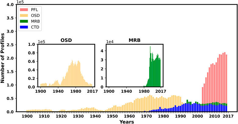
FIGURE 2. Number of profiles from the four measuring platforms used in this study and extracted from WOD18: Ocean Station Data (OSD); Moored Buoys (MRB); Conductivity Depth Temperature (CTD); and Profiling Floats (PFL).

2.1 Additional Quality Control Procedure

WOD implements two types of quality control checks, represented by different quality flags: first an individual value flag (WODf) for each measured point in the vertical for checking systematic errors in the observations; and second a profile flag (WODfp) that denotes a statistical quality check, as explained in Locarnini et al. (2019). In the following text, WODf and WODfp are together referred to as WOD QC. Uncertainties in the ocean historical observations are sum of gross errors and representativeness errors as pointed by Janjić et al. (2018) and Cowley et al. (2021) which defined it as Type A and Type B uncertainty. A more sophisticated automated quality control procedures has been achieved during the last years by the International Quality-Controlled Ocean Database (IQuOD) v0.1. Further IQuoD v0.1 contains only temperature profiles with the uncertainty estimate of gross error (Type A) while quality control of representativeness error (Type B) was out of the scope of the project as mentioned by Cowley et al. (2021). Therefore, we felt there is a need of Additional QC (AQC) to remove the observations containing representativeness error (Type B) and we implemented it as follow:

i) The domain is divided into 5 × 5° boxes, where mean and standard deviations (std) are computed and used as thresholds in step (ii).

ii) Data outside 2 std in each box is eliminated and the procedure is repeated until convergence is achieved, which is denoted when no data are greater in value than the std level.

The AQC is iterative, unlike the WOD QC, and it is applied after the WOD QC is considered. The numbers of observations before and after the application of the AQC are given in Figure 3. Distribution of salinity observations (January) at surface before and after the application of AQC are shown in Supplementary Figure S5 in supplementary material. The application of AQC has eliminated the observations with representative error which were still present with WOD18, i.e. (WODf and WODfp) QC. The application of AQC eliminates less than 15% of the total profiles.

FIGURE 3

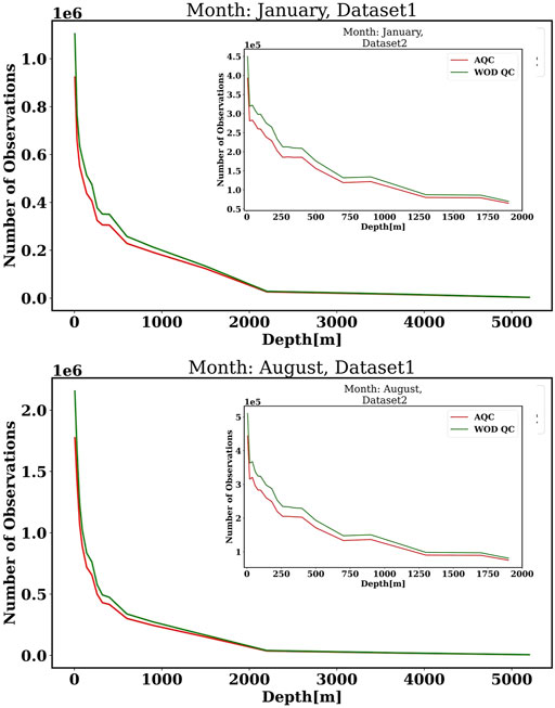
FIGURE 3. Number of observations (Temperature) using WOD QC and AQC for Dataset1 and Dataset2: January (top); August (bottom).

3 Interpolation Scheme

DIVAnd is based on the Variational Inverse Method (VIM) and applied on a curvilinear orthogonal grid using a finite difference scheme (Barth et al., 2014). This method is equivalent to Optimal Interpolation (OI), and the main difference between DIVAnd and OI is in the consideration of land boundaries, as explained in the introduction.

In DIVAnd, the cost function is minimised and contains three terms: the misfit between the observations and the reconstructed Field; the regularity or smoothness constraint; and the advection constraint. This cost function can be written as:

$J[\varphi ]=\sum _{i=1}^N{\mu }_{\mathrm{i}}{[d_{\mathrm{i}}-\phi (x_{\mathrm{i}},y_{\mathrm{i}})]}^2+\Vert \phi -{\phi }_{\mathrm{b}}{\Vert }^2+J_{\mathrm{c}}(\phi ),(1)$

where d_i are the observations at the location (x_i, y_i), φ is the target field in the regular grid, or the analysis, φ_b is the first guess field or “background” and μ_i are weights derived from specific error estimates (Troupin et al., 2012) and the correlation length L, which are described later. J_c is the advection constraint, in which variable gradients are assumed along the coasts only, thus imposing no normal flux of temperature and salinity across land-sea boundaries. The smoothness constraint is defined as:

$\Vert \phi -{\phi }_{\mathrm{b}}{\Vert }^2={\alpha }_2{\int }_{\mathrm{\Omega }}(\nabla \nabla \phi :\nabla \nabla \phi +{\alpha }_{\mathrm{1}}\nabla \phi .\nabla \phi +{\alpha }_{\mathrm{0}}{\phi }^2)d\mathrm{\Omega },(2)$

The non-dimensional form of the cost function is:

$\tilde{J}[\varphi ]=\sum _{i=1}^N{\mu }_{\mathrm{i}}{L}^2{[d_{\mathrm{i}}-\phi (x_{\mathrm{i}},y_{\mathrm{i}})]}^2+{\int }_{\tilde{\mathrm{\Omega }}}(\tilde{\nabla }\tilde{\nabla }\phi :\tilde{\nabla }\tilde{\nabla }\phi +{\alpha }_{\mathrm{1}}{L}^2\tilde{\nabla }\phi .\tilde{\nabla }\phi +{\alpha }_{\mathrm{0}}{L}^4{\phi }^2)d\tilde{\mathrm{\Omega }}+J_{\mathrm{c}}(\phi ),(3)$

: is generalisation of the scalar product of two vectors and is defined as

$\nabla \nabla \phi :\nabla \nabla \phi =\sum _i\sum _j({\partial }^2\phi /\partial x_i\partial x_j)({\partial }^2\phi /\partial x_i\partial x_j).(4)$

In DIVAnd the following values are assumed:

$\begin{array}{ccc}\hfill {\alpha }_0{L}^4& =\hfill & 1\hfill \\ \hfill {\alpha }_1{L}^2& =\hfill & 2\hfill \\ \hfill {\alpha }_2& =\hfill & 1\hfill \\ \hfill {\mu }_i{L}^2& =\hfill & 4\pi \frac{{\sigma }^2}{{ϵ}_i^2}\hfill \end{array}(5)$

Equation 5 shows that μ is defined as the ratio of signal variance σ², which is considered the background error variance of the observations, ${ϵ}_i^2$. For more details of the solution method, see Barth et al. (2014).

The best estimate or analysis depends on the values of two key parameters, the correlation length L and the Noise to Signal ratio (N/S), i.e., $\frac{1}{{\mu }_i}$Eq. 5. Large values of the correlation length indicate a larger number of weighted average observations in the estimate of the field at each grid point, resulting in a smoother field, while smaller values will allow for smaller-scale feature resolution, resulting in a noisier field.

Large N/S of imply larger analysis field deviations from the observations, or conversely, the analysis field is closer to the background field. However, small values of N/S mean that the analysis field is closer to the observations relative to the first guess field. We denote this parameter to always be less than one so the observations are more important than the background. As discussed in the following sections, the importance of the background is limited in our analysis due to the AQC used.

3.1 Horizontal and Vertical Analysis Domain

The global domain for the analysis extends from 0°E to 360°W and from 80°N to −80°S. The grid spacing is $\frac{1}{4}°$ in latitude and longitude. The bathymetry is specified from the GEBCO 30” data (IOC and IHO, 2003). We consider 45 (surface to 6000m) and 36 (surface to 2000m) non-uniform depth layers in this analysis for SDC_V1 and SDC_V2, respectively, as listed in Table 2.

TABLE 2

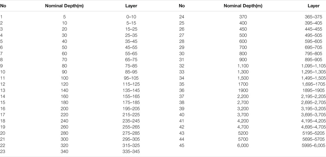
TABLE 2. Depth layers used for SDC climatology: the nominal depth is selected at the middle of each layers. The levels for SDC_V1 extend from 5 m to 6,000 m and for SDC_V2 from 5 to 2000 m.

We considered a vertical discretization consisting of 10 m layers around the nominal vertical depth of the analysis, as reported in Table 2. This prevents vertical smearing of the vertical temperature and salinity gradients, and unrealistic thermocline and halocline results being obtained. In addition, we avoid the use of data far from the interpolation level as the profiles may have vertical data gaps.

To better resolve the upper thermocline structure, a larger number of layers are defined from the surface to 500 m, and the remaining levels are at distances of 100 m between 500 m and 1900 m depth and of 500 m between 1900 m and 6,000 m. Data are grouped in monthly time steps and all data collected during the month contribute equally to the estimate of the monthly climatology.

3.2 Background Fields

The choice of the first guess field or background field may be important when data are irregularly spaced both horizontally and vertically. Two types of backgrounds were tested in this study. The first, Background1, is a vertical profile corresponding to a spatial mean of observations over the entire global ocean (Figure 4) for Dataset1. The second, Background2, is estimated by using the DIVAnd obtained from Background1, a correlation length of 1,000 km and a N/S ratio of 0.5. Similarly to Background1 several authors have taken zonal averages of observations and used it as first guess for climatologies (Levitus, 1982). However, averaging water masses across the deep portions of different ocean basins that are completely disconnected on the timescales of 100 years give rise to high standard deviations in deep waters. Notwithstanding these limitations and the simplicity of the first guess, the use of DIVAnd and AQC makes the analysis quite insensitive to the background as shown below. We select the background according to the computed climatology residuals, calculated as:

$r^i(x{o}_{\alpha },y{o}_{\beta },z_{\gamma })=H({{\theta }^i}_{\mathrm{c}}(x_k,y_j,z_p))-y_o(x{o}_{\alpha },y{o}_{\beta },z_{\gamma })(6)$

where (x_k, y_j, z_p) are the m, n, q grid points of the three dimensional interpolating grid, respectively, y_o(xo_α, yo_β, zo_γ) are the observations at α, β, γ points and ${\theta }_c^i$ is the i − th climatology under consideration. H is the bilinear interpolation or observational operator that interpolates the climatology to the observational point. rⁱ is clearly an estimate of the error of the climatology at the observational grid points, due to the smoothing carried out by the interpolation scheme and all of the assumptions within the numerical scheme.

FIGURE 4

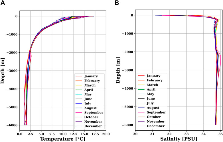
FIGURE 4. Background1(spatial mean of data at each layer) for SDC_V1 computed from Dataset1: Temperature (A); and Salinity (B).

Figures 5A,B show the Root Mean Squares(RMS) of residuals of the SDC_V1 analysis conducted using Background1 and the WOD QC. Figures 5C,D shows the difference of the residuals between the climatologies computed with Background2 and Background1. The difference is visible and quantitatively significant.

FIGURE 5

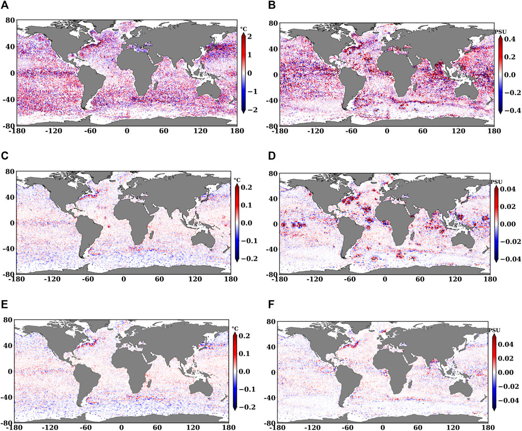
FIGURE 5. Residual and residuals difference for Temperature (A,C, E) and Salinity (B,D,F) at 5 m using WOD QC with choice of Background1. RMS of residuals in (A) 0.69°C, and (B) 0.94PSU. Difference of residuals with Background2 and Background1 using WOD QC, RMS of residuals in (C) 0.02°C, and (D) 0.03PSU. Difference of residuals of Background2 and Background1 using AQC, RMS of residuals in (E) 0.02°C, and (F) 0.01PSU.

However, when AQC is used, as shown in Figures 5E,F the background does not appreciably change the climatological estimate. The AQC eliminates outliers or non-representative data, which reduces the sensitivity of the analysis to the background specification. The quality of the input dataset determines the influence of the background on the estimate: if only the WOD QC input dataset is used, i.e., outliers/non-representative data are left in, the choice of background becomes more important and the difference between residuals using different backgrounds is large, particularly for salinity. Thus, we conduct our analysis for both Dataset1 and Dataset2 with Background1.

3.3 Sensitivity Experiments for DIVAnd Parameter Choices

Selecting the correlation lengths L and N/S for a global ocean domain is challenging. The global ocean contains a multiplicity of scales. Therefore, a single L value could either overly smear the general circulation fronts (such as the western boundary currents) or contaminate the climatology with mesoscale eddies or other higher frequency processes. L has previously been estimated using the data itself, by binning the data and fitting analytical curves (Nittis et al., 1993). However, in the global ocean the data is so non-uniformly spaced that the L estimation quality of different ocean areas will be very different. Thus, we take a new view of the traditional approach and use equal L values for every location, as in WOA18 (Locarnini et al., 2019).

We conducted several sensitivity experiments to select reasonable values using L values ranging from 100 to 1,000 km and N/S values from 0.1 to 50.

A roughness index is defined as the mean of the derivative of field in the two directions as:

$RI=\frac{1}{N}\sum _{i,j=1}^{n,m}\sqrt{{({\mathrm{\Delta }}_{{\mathrm{x}}_{\mathrm{i}}}f)}^2+{({\mathrm{\Delta }}_{{\mathrm{y}}_{\mathrm{j}}}f)}^2}(7)$

where Δ is the finite difference derivative in the latitudinal and longitudinal directions, x_i is the grid spacing in the longitudinal direction and y_j in the latitudinal direction, and N = n ∗ m is the total number of the interpolating grid points.

RI gives a measure of the spatial scale of the field. For example, a field with mesoscale features will have high RI values while a smoother field with large-scale features will have low values. We do not find that using the Rossby radius of deformation and/or its corresponding wavelength can correctly define the correlation length for a climatology. The correlation length is the result of many propagating waves in the ocean, which combine to form a mean field that is necessarily smooth. Thus, a roughness index or its inverse, a smoothness index, is a better choice for establishing the correlation length of the interpolating algorithm in terms of the wavelength of the primary process that creates the climatology. Many climate indices are in fact “smoothed” to extract basic long-term signals.

As expected, for large L values the analysis gives a small RI value, as shown in Figure 6. We also establish that the RI should not exceed the standard deviation (std) of the data itself, as shown by the dotted blue line in Figure 6. The criteria of accepting a value of RI less than the field STD evidently only eliminates L at 100 km, varying slightly with depth. The “elbow” of all of the curves lies between 0.4 and 0.6 for the N/S ratio, and thus we select 0.5. When selecting this N/S value and taking an RI equal to approximately half of the field STD, we obtain a value for L of 300 km.

FIGURE 6

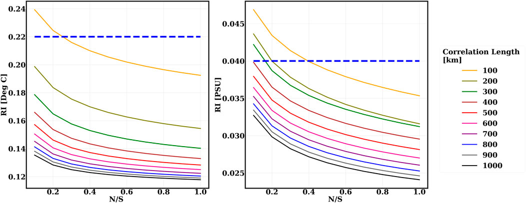
FIGURE 6. Roughness Index of SDC_V1: Temperature (left) and Salinity (right) for January at 5m for different CL and N/S (dotted blue line represents the standard deviation of in-situ observations).

4 Discussion

We conducted temperature and salinity mapping with a correlation length of 300 km and an N/S of 0.5 for Dataset1 and Dataset2 for all depths and months. Figure 7 shows the mapped temperature and salinity fields for Dataset1 for January at different depth levels. The fields are masked if the analysis errors are greater than 30% (relative to the field standard deviation). We find that the Pacific area still suffers from a scarcity of data, in addition to the deep ocean.

FIGURE 7

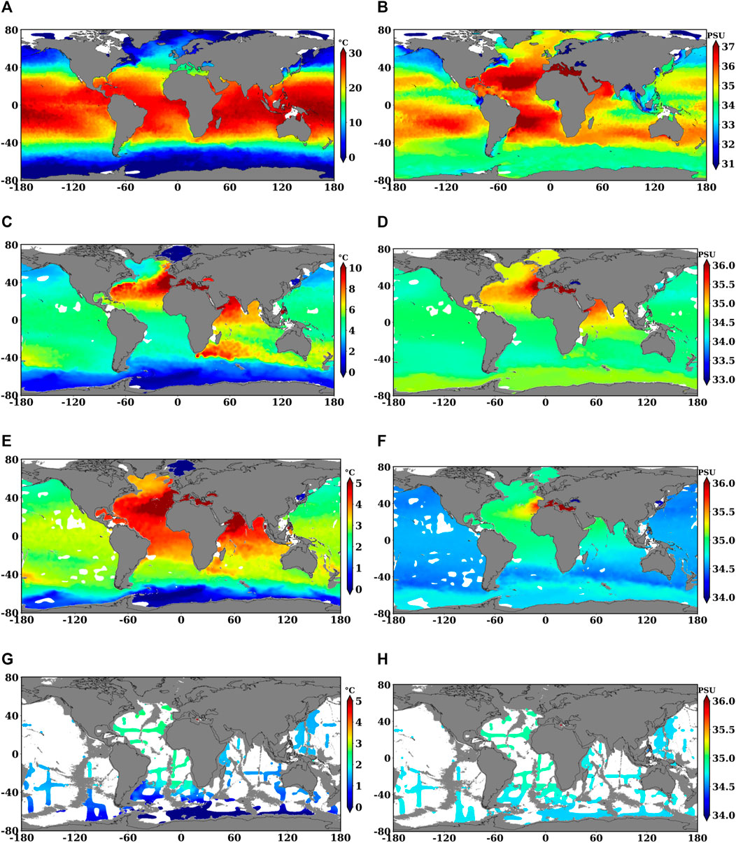
FIGURE 7. Temperature (A,C,E,G) and Salinity (B,D,F,H) climatology for January at 5m, 900m, 1050m and 3700m, respectively, from SDC_V1.

SDC_V1 is a longer-term average while SDC_V2 is an estimate of the last 15 years. The difference between these two estimates is shown in Figure 8. SDC_V2 is warmer and more saline than SDC_V1, and the root mean square (RMS) difference varies from 0.4° to 0.5 °C and 0.7 to 0.6 PSU for temperature and salinity, respectively. To better quantify the sign of the differences we computed the global mean bias of salinity and temperature in Figure 9. The negative mean bias at the surface indicates that SDC_V2 is less saline than SDC_V1. This might be due to the last 15 years (2003–2017) increase of freshening of surface waters with respect to the (1900–2017) time period. However such freshening does not go subsurface due to buoyancy effects. In the subsurface at the contrary, SDC_V2 is more saline than SDC_V1 and we argue that this is allowed by compensating effects between high tempratures and high salt in the equation of state, as described by Chen et al. (2019).

FIGURE 8

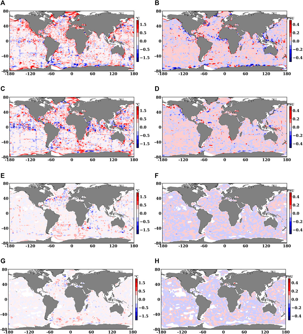
FIGURE 8. January mapping differences between SDC_V2 and SDC_V1 for Temperature with RMSD (A) 0.4°C, (C) 0.39°C, (E) 0.08 °C, (G) 0.04 °C, and Salinity with RMSD (B) 0.66PSU, (D) 0.05PSU, (F) 0.01PSU, and (H) 0.01PSU at 5m, 100m, 900m and 1500m, respectively.

FIGURE 9

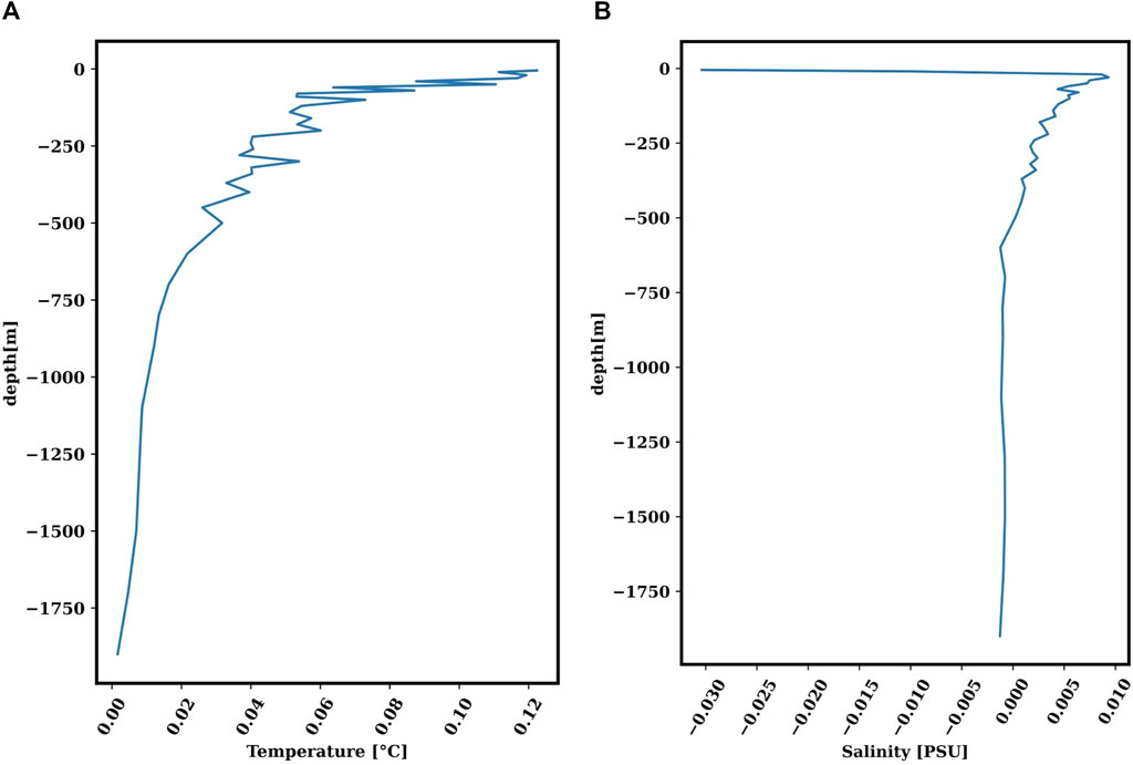
FIGURE 9. Global mean bias profile (difference between SDC_V2 and SDC_V1) for (A) Temperature and (B) Salinity during January.

4.1 Validation Using Other Climatologies

Validating the analysis is an essential step, as it indicates the reliability of the results. We validate our results using the WOA18 and WAGHC (isobarically averaged version) climatological estimates because they have similar interpolating grids at 1/4° resolution. Other climatologies might exist but at lower space and time resolution. The main source of data in WAGHC is from WOD13, and in particular OSD, CTD, PFL and APB. Additional data were obtained from the Alfred Wegener Institute, Bremerhaven, and from various institutions in Canada for the period between 1900 and 2016 (Gouretski, 2018). The data considered in WOA18 are profiles from OSD, CTD, PFL, MRB, Mechanical Bathythermographs, Digital Bathythermographs, Expendable Bathythermographs, moored and drifting buoys, gliders, undulating oceanographic recorders (UOR), pinniped mounted CTD sensors and surface-only data (Locarnini et al., 2019) and (Zweng et al., 2019). WOA18 monthly climatology is computed from surface to 1500 m on 22 depth levels at a spatial resolution of 0.25 over the 6 decades of 1955–1964, 1965–1974, 1975–1984, 1985–1994, 1995–2004 and 2005–2012. While seasonal fields are computed for deeper depth from surface to 6000 m on 57 depth levels. We understand the climatologies are done for different periods but we argue that a comparison is a first step to check consistency between them.

To compute the differences between the climatologies, we interpolated the WOA18 time average fields over the 6 decades on the DIVAnd analysis grid using linear interpolation, and similarly for WAGHC. Supplementary Figures S1–S4 in the supplementary material show that differences are localised and are maximum in dynamically active regions such as along the Gulf Stream, the South equatorial current, the Gulf of Guinea, the Bay of Bengal, etc. Moreover, largest differences are found in the Arctic region that might be mainly due to different observational data sets used. We have also added several Supplementary Tables S1–S14 in the supplementary material evaluating the BIAS and the RMSD of salinity and temperature computed as the spatial average of the differences between the climatologies in different layers for the equatorial regions (-10°S to 10°N), north and south Atlantic, Pacific (11°N to 80 °N) and (-80°S to -9°S), respectively, and Indian Ocean (20°N to -40°S). SDC_V1 has a positive bias with respect to WOA and a negative bias for WAGHC for both temperature and salinity at all the depths in all regions. Maximum differences are found at surface and thermocline depths. Further, larger temperature differences are noticed in the north and south Atlantic, and Indian ocean for WOA, while WAGHC has maximum differences in the north Atlantic region. Maximum temperature differences are found in equatorial Atlantic and Pacific for WOA while for WAGHC maximum RMSD is found in Atlantic ocean. Overall, the comparison of RMSD values shows larger differences for both temperature and salinity with WOA as compared to WAGHC that is probably due to the fact the interpolation scheme SDC and WAGHC are similar.

Moreover, Hovmoller diagram was constructed for the horizontal spatial average of the RMS differences between WOA18 and WAGHC. Figure 10 shows that the largest RMS temperature differences are found with SDC_V1 at the thermocline depth for both WOA18 and WAGHC, but the differences are more prominent with WOA18. We argue that this difference at the thermocline is due to the different interpolations of the observational profiles at the levels, which create potential anomalies or simply different data being used. The differences in salinity are greater in the surface layer and for the summer months, probably due to the different number of profiles used.

FIGURE 10

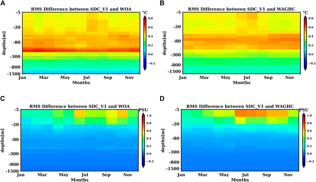
FIGURE 10. Hovmoller diagram of the root mean square difference between SDC_V1 and WOA for (A,C) and SDC_V1 and WAGHC for (B,D). Left panels give temperature and right panels salinity.

4.2 Ensemble Mean Climatology

In the previous section we reveal some of the differences between the four climatological estimates. Such uncertainties are due to the characteristics of the selected input dataset, the specific background and statistical interpolation algorithms, and the type of quality control applied. As for numerical models, a multi-model statistical estimate can reduce the errors of specific quality assessment indices. Thus, a diverse combination of climatological estimating methods can provide the best estimate of the climatological state of the ocean. Ensemble methodologies have been proposed in the past for the reconstruction of atmospheric temperatures (Krishnamurti et al., 1999) and for climatologies of global ocean salinities (Liu et al., 2020). Furthermore it is well knwon that ensemble mean is a commonly used post-processing methodology for reanalyses (Frankcombe et al., 2018) and climate projections (Solomon et al., 2007). In these works, it is shown that the ensemble mean is a statistically better estimate of the truth, so we have applied this to the different global ocean climatologies. The multi-model ensemble mean will reduce the uncertainties associated with the statistical ensemble mean estimate. Our multi-model ensemble climatology is the ensemble mean of four climatologies WOA, WAGHC, and SDC_V1 and SDC_V2. Each member of the ensemble is considered to be a different climatology derived from a different statistical interpolating model, and the ensemble mean of these models should be superior to that of any of the single models within a particular evaluation score (Krishnamurti et al., 1999). The evaluation score applied is derived from the comparison between the ensemble mean residual and each single climatology residual.

The climatology multi-model ensemble mean, ${\theta }_{\mathrm{c}}^E(x,y,z)$ is defined as:

${\theta }_{\mathrm{c}}^E(x,y,z)=\sum _{i=1}^N\frac{{{\theta }^i}_{\mathrm{c}}(x,y,z)}{N},(8)$

The residual defined in Eq. 6 contains various sources of errors in addition to the difference between the climatology and the observations. We assume first that the climatological estimate is the sum of true climatological value and the interpolation errors, so-called ϵ_H:

$H({{\theta }^i}_{\mathrm{c}}(x_k,y_j,z_p))=H{({{\theta }^i}_{\mathrm{c}}(x_k,y_j,z_p))}^T+{ϵ}_{\mathrm{H}}.(9)$

Moreover, the observations itself are sum of true observational values and errors, ϵ_o:

$y_o(x{o}_{\alpha },y{o}_{\beta },z_{\gamma })=y_o{(x{o}_{\alpha },y{o}_{\beta },z_{\gamma })}^T+{ϵ}_{\mathrm{o}},(10)$

Finally, the residuals in the Eq. 6 can now be decomposed as follows:

$r^i(x{o}_{\alpha },y{o}_{\beta },z_{\gamma })=H{({{\theta }^i}_{\mathrm{c}}(x_k,y_j,z_p))}^T+{ϵ}_{\mathrm{H}}-y_o{(x{o}_{\alpha },y{o}_{\beta },z_{\gamma })}^T-{ϵ}_{\mathrm{o}}(11)$

Thus the residuals are the sum of the differences between the true climatology and the true observational values plus the two different types of errors. We call this synthetically residual errors. A lower residual error is not a necessary condition for a high quality climatology but we argue that it is a sufficient criteria. A climatological estimate with lower residual will be considered as a better estimate.

The resulting vertical profile is denoted by $\tilde{r}(z)$ and is defined as:

${\tilde{r}}^i(z_{\gamma })=\sqrt{\sum _{\alpha ,\beta =1}^{M,L}\frac{{(r^i(x{o}_{\alpha },y{o}_{\beta },z_{\gamma })-{\bar{r}}^i(z_l))}^2}{M\ast L}}.(12)$

where M ∗ L is the number of horizontal observational grid points.

Figure 11 shows the ${\tilde{r}}^i$. The ensemble residual STD is the second lowest, confirming that the multi-model ensemble mean is a good estimate of the climatology. The lowest values are achieved by SDC_V1, but we argue that this is due to the fact that we computed the residuals directly from the dataset used to generate the SDC_V1 climatology.

FIGURE 11

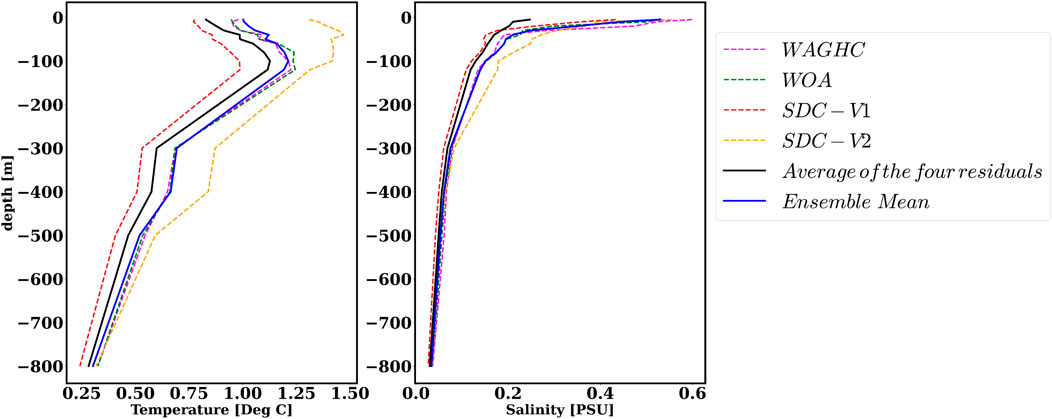
FIGURE 11. Standard deviation of anomaly residuals ${\tilde{r}}^i$ for available climatological estimates (${{\theta }^i}_{\mathrm{c}}$) (dashed lines), average of the four residuals (continuous blue line) and standard deviation of ensemble mean climatology residuals (black continuous line).

5 Summary and Future Work

Two versions of a global ocean climatology for temperature and salinity were estimated using a new interpolation scheme, DIVAnd, which enables a better assessment of coastal constraints. We demonstrated that an additional quality control is required to produce a good quality climatology. Two backgrounds were analyzed: a spatial mean of observations in the horizontal and an analysis conducted with a very large correlation length of 1000 km and N/S of 0.5. The results show that if pre-processing is carried out using the AQC procedure, the resulting analysis field is less dependent on the choice of the background field (see Figure 5).

In addition, ours is the first study in which the selection of DIVAnd parameters is deduced from a new roughness index (RI), which quantifies the degree of smoothness of the analysis as a function of the correlation length and N/S values.

When comparing the SDC_V1 climatology with WOA and WAGHC we find reasonable agreement, but also significant differences in terms of the thermocline and surface layers. The SDC_V1 climatology is closer to WAGHC than WOA18 in terms of both temperature and salinity. One reason could be connected to the fact that the OA parameters used and the technique itself are similar to DIVAnd. Currently available historical datasets enable an almost complete reconstruction of the global ocean fields. However, data gaps still exist, and differences among interpolation schemes and input dataset quality control lead to significant uncertainties in the climatological estimates. For the first time, we have demonstrated that a multi-model ensemble of different climatologies can produce low residual error compared to each single climatological estimate.

Future work can consider the application of the improved quality control procedure developed in Shahzadi et al. (2021) using a regime-oriented division instead of regular 5° square rectangles in a global domain. An optimised choice of DIVAnd parameters that are different for each level may improve the results. A validation with independent datasets such as satellite observations or a randomly subsampled input dataset will enable an assessment of whether the analysis under- or over-fits the observations. Further as pointed by Lozier et al. (1994), an isopycnal climatology using DIVAnd is required to avoid the artificial mixing water masses.

Data Availability Statement

The datasets presented in this study can be found in online repositories. The names of the repository/repositories and accession number(s) can be found below: https://doi.org/10.12770/98d22ac0-5398-4889-8f8e-8f28273b548b.

Author Contributions

KS wrote the text and created the figures in the paper. NP corrected and wrote parts of the sections, and in particular contributed to the conceptual framing of the work. VL helped assess the structure of the WOD dataset in the early stages of the quality control algorithm, and AB and CT help with the application of the DIVAnd interpolation scheme. SS assisted in revising the content of the PhD thesis that served as the basic material for this article.

Funding

The study was fully funded by the European project Horizon2020 SeaDataCloud - Further developing the pan-European infrastructure for marine and ocean data management Grant Agreement Number: 730960 and is part of the PhD thesis of KS at the University of Bologna. NP was additionally funded by the University of Bologna.

Conflict of Interest

The authors declare that the research was conducted in the absence of any commercial or financial relationships that could be construed as a potential conflict of interest.

Publisher’s Note

All claims expressed in this article are solely those of the authors and do not necessarily represent those of their affiliated organizations, or those of the publisher, the editors and the reviewers. Any product that may be evaluated in this article, or claim that may be made by its manufacturer, is not guaranteed or endorsed by the publisher.

Acknowledgments

We thank Dr. Tim Boyer, NOAA (United States) reviewer of the PhD thesis, who suggested important improvements.

Supplementary Material

The Supplementary Material for this article can be found online at: https://www.frontiersin.org/articles/10.3389/fenvs.2021.711363/full#supplementary-material

Footnotes

¹https://www.nodc.noaa.gov/OC5/WOD/pr_wod.html.

References

Barker, P. M., Dunn, J. R., Domingues, C. M., and Wijffels, S. E. (2011). Pressure Sensor Drifts in Argo and Their Impacts. J. Atmos. Oceanic Technology 28, 1036–1049. doi:10.1175/2011jtecho831.1

CrossRef Full Text | Google Scholar

Barnes, S. L. (1964). A Technique for Maximizing Details in Numerical Weather Map Analysis. J. Appl. Meteorol. 3, 396–409. doi:10.1175/1520-0450(1964)003<0396:atfmdi>2.0.co;2

CrossRef Full Text | Google Scholar

Barth, A., Beckers, J.-M., Troupin, C., Alvera-Azcárate, A., and Vandenbulcke, L. (2014). divand-1.0: N-Dimensional Variational Data Analysis for Ocean Observations. Geosci. Model. Dev. 7, 225–241. doi:10.5194/gmd-7-225-2014

CrossRef Full Text | Google Scholar

Brasseur, P. P. (1991). A Variational Inverse Method for the Reconstruction of General Circulation fields in the Northern Bering Sea. J. Geophys. Res. 96, 4891–4907. doi:10.1029/90jc02387

CrossRef Full Text | Google Scholar

Bretherton, F. P., Davis, R. E., and Fandry, C. B. (1976). A Technique for Objective Analysis and Design of Oceanographic Experiments Applied to Mode-73. Deep Sea Research and Oceanographic Abstracts, 23. Elsevier, 559–582. doi:10.1016/0011-7471(76)90001-2

CrossRef Full Text | Google Scholar

Chen, L., Huang, J. G., Ma, Q., Hänninen, H., Tremblay, F., and Bergeron, Y. (2019). Long‐term Changes in the Impacts of Global Warming on Leaf Phenology of Four Temperate Tree Species. Glob. Change Biol. 25, 997–1004. doi:10.1111/gcb.14496

PubMed Abstract | CrossRef Full Text | Google Scholar

Cowley, R., Killick, R., Boyer, T., Gouretski, V., Reseghetti, F., Kizu, S., et al. (2021). International Quality-Controlled Ocean Database (Iquod) V0. 1: the Temperature Uncertainty Specification. Front. Mar. Sci. 8, 607. doi:10.3389/fmars.2021.689695

CrossRef Full Text | Google Scholar

Daley, R. (1993). Atmospheric Data Analysis, 2. Cambridge University Press.

Frankcombe, L. M., England, M. H., Kajtar, J. B., Mann, M. E., and Steinman, B. A. (2018). On the Choice of Ensemble Mean for Estimating the Forced Signal in the Presence of Internal Variability. J. Clim. 31, 5681–5693. doi:10.1175/jcli-d-17-0662.1

CrossRef Full Text | Google Scholar

Gandin, L. (1960). On Optimal Interpolation and Extrapolation of Meteorological fields. Trudy GGO 114, 75–89.

Google Scholar

Garcia, H., Boyer, T., Locarnini, R., Baranova, O., and Zweng, M. (2018). World Ocean Database 2018: Users Manual (Prerelease). NOAA Atlas NESDIS81.

Gouretski, V. (2019). A New Global Ocean Hydrographic Climatology. Atmos. Oceanic Sci. Lett. 12, 226–229. doi:10.1080/16742834.2019.1588066

CrossRef Full Text | Google Scholar

Gouretski, V. (2018). World Ocean Circulation Experiment - Argo Global Hydrographic Climatology. Ocean Sci. 14, 1127–1146. doi:10.5194/os-14-1127-2018

CrossRef Full Text | Google Scholar

IOC and IHO (2003). Bodc: Centenary Edition of the Gebco Digital Atlas, Published on Cd-Rom on Behalf of the Intergovernmental Oceanographic Commission and the International Hydrographic Organization as Part of the General Bathymetric Chart of the Oceans. Liverpool, UK: British Oceanographic Data Centre.

Janjić, T., Bormann, N., Bocquet, M., Carton, J., Cohn, S., Dance, S., et al. (2018). On the Representation Error in Data Assimilation. Quart. J. R. Meteorol. Soc., 144. doi:10.1002/qj.3130

Jia, W., Wang, D., Pinardi, N., Simoncelli, S., Storto, A., and Masina, S. (2016). A Quality Control Procedure for Climatological Studies Using Argo Data in the north pacific Western Boundary Current Region. J. Atmos. Oceanic Technology 33, 2717–2733. doi:10.1175/jtech-d-15-0140.1

CrossRef Full Text | Google Scholar

Krishnamurti, T. N., Kishtawal, C. M., LaRow, T. E., Bachiochi, D. R., Zhang, Z., Williford, C. E., et al. (1999). Improved Weather and Seasonal Climate Forecasts from Multimodel Superensemble. Science 285, 1548–1550. doi:10.1126/science.285.5433.1548

PubMed Abstract | CrossRef Full Text | Google Scholar

Levitus, S. (1982). Climatological Atlas of the World Ocean, NOAA Professional Paper No. 13. US Department of Commerce.

Liu, C., Liang, X., Chambers, D. P., and Ponte, R. M. (2020). Global Patterns of Spatial and Temporal Variability in Salinity from Multiple Gridded Argo Products. J. Clim. 33, 8751–8766. doi:10.1175/jcli-d-20-0053.1

CrossRef Full Text | Google Scholar

Locarnini, M., Mishonov, A., Baranova, O., Boyer, T., Zweng, M., Garcia, H., et al. (2019). Temperature, World Ocean Atlas 2018. NOAA Atlas NESDIS81. Available online at https://accession.nodc.noaa.gov/NCEI-WOA18

Google Scholar

Lozier, M. S., McCartney, M. S., and Owens, W. B. (1994). Anomalous Anomalies in Averaged Hydrographic Data. J. Phys. Oceanogr. 24, 2624–2638. doi:10.1175/1520-0485(1994)024<2624:aaiahd>2.0.co;2

CrossRef Full Text | Google Scholar

Nittis, K., Pinardi, N., and Lascaratos, A. (1993). Characteristics of the Summer 1987 Flow Field in the Ionian Sea. J. Geophys. Res. 98, 10171–10184. doi:10.1029/93jc00451

CrossRef Full Text | Google Scholar

Owens, W. B., and Wong, A. P. S. (2009). An Improved Calibration Method for the Drift of the Conductivity Sensor on Autonomous CTD Profiling Floats by θ-S Climatology. Deep Sea Res. Oceanographic Res. Pap. 56, 450–457. doi:10.1016/j.dsr.2008.09.008

CrossRef Full Text | Google Scholar

Solomon, S., Manning, M., Marquis, M., and Qin, D. (2007). Climate Change 2007-the Physical Science Basis: Working Group I Contribution to the Fourth Assessment Report of the IPCC (Vol. 4). Cambridge University Press.

Shahzadi, K., Pinardi, N., and Lyubartsev, V. (2021). A Non-linear Quality Control Procedure for Representativeness Errors in Ocean Historical Datasets. Bollettino di Geofisica 12, 99.

Google Scholar

Shahzadi, K., Pinardi, N., Lyubartsev, V., Zavatarelli, M., and Simoncelli, S. (2020). SeaDataCloud Temperature and Salinity Climatologies for the Global Ocean V2). ITALY. Report (scientific report). doi:10.13155/77512

Simoncelli, S., Coatanoan, C., Myroshnychenko, V., Bäck, Ö., Sagen, H., Scory, S., et al. (2021). Seadatacloud Data Products for the European Marginal Seas and the Global Ocean. Available online at: http://hdl.handle.net/2268/259074 .

Google Scholar

Troupin, C., Barth, A., Sirjacobs, D., Ouberdous, M., Brankart, J.-M., Brasseur, P., et al. (2012). Generation of Analysis and Consistent Error fields Using the Data Interpolating Variational Analysis (Diva). Ocean Model. 52-53, 90–101. doi:10.1016/j.ocemod.2012.05.002

CrossRef Full Text | Google Scholar

Wong, A. P. S., Johnson, G. C., and Owens, W. B. (2003). Delayed-Mode Calibration of Autonomous CTD Profiling Float Salinity Data Byθ-SClimatology*. J. Atmos. Oceanic Technol. 20, 308–318. doi:10.1175/1520-0426(2003)020<0308:dmcoac>2.0.co;2

CrossRef Full Text | Google Scholar

Zweng, M., Seidov, D., Boyer, T., Locarnini, M., Garcia, H., Mishonov, A., et al. (2019). Salinity, World Ocean Atlas 2018. NOAA Atlas NESDIS81. Available online at: https://accession.nodc.noaa.gov/NCEI-WOA18

Google Scholar