On the Treatment of Soil Water Stress in GCM Simulations of Vegetation Physiology

Current land surface schemes in weather and climate models make use of the so-called coupled photosynthesis–stomatal conductance (A–g_s) models of plant function to determine the surface fluxes that govern the terrestrial energy, water and carbon budgets. Plant physiology is controlled by many environmental factors, and a number of complex feedbacks are involved, but soil moisture control on root water uptake is primary, particularly in sub-tropical to temperate ecosystems. Land surface models represent plant water stress in different ways, but most implement a water stress factor, β, which ranges linearly (more recently also curvilinearly) between β = 1 for unstressed vegetation and β = 0 at the wilting point, expressed in terms of volumetric water content ($\theta$). $\beta$ is most commonly used to either limit A or g_s, and hence carbon and water fluxes, and a pertinent research question is whether these treatments are in fact interchangeable. Following Egea et al. (Agricultural and Forest Meteorology, 2011, 151 (10), 1,370–1,384) and Verhoef et al. (Agricultural and Forest Meteorology, 2014, 191, 22–32), we have implemented new β treatments, reflecting higher levels of biophysical complexity in a state-of-the-art LSM, Joint UK Land Environment Simulator, by allowing root zone soil moisture to limit plant function non-linearly and via individual routes (carbon assimilation, stomatal conductance, or mesophyll conductance) as well as any (non-linear) combinations thereof. The treatment of β does matter to the prediction of water and carbon fluxes: this study demonstrates that it represents a key structural uncertainty in contemporary LSMs, in terms of predictions of gross primary productivity, energy fluxes and soil moisture evolution, both in terms of climate means and response to a number of European droughts, including the 2003 heat wave. Treatments allowing ß to act on vegetation fluxes via stomatal and mesophyll routes are able to simulate the spatiotemporal variability in water use efficiency with higher fidelity during the growing season; they also support a broader range of ecosystem responses, e.g., those observed in regions that are radiation limited or water limited. We conclude that current practice in weather and climate modelling is inconsistent, as well as too simplistic, failing to credibly simulate vegetation response to soil water stress across the typical range of variability that is encountered for current European weather and climate conditions, including extremes of land surface temperature and soil moisture drought. A generalized approach performs better in current climate conditions and promises to be, based on responses to recently observed extremes, more trustworthy for predicting the impacts of climate change.

Introduction

Water availability exerts a major control on vegetation gross primary productivity (GPP), as well as on the land surface energy balance. It has been estimated that ∼40% of the global vegetated land surface, particularly in sub-humid, semi-arid, and arid regions (Stocker et al., 2018; O'Sullivan et al., 2020), experiences plant activity/growth limitations caused by seasonal water deficits (Nemani et al., 2003; Beer et al., 2010). In the context of future projections of ecosystem response, soil moisture stress is predicted to increase over large regions (Berg et al., 2016; Ukkola et al., 2020). Consequently, there is a clear requirement to incorporate accurate, process-based models of plant response to soil moisture stress in coupled land-atmosphere climate models. However, the models currently used to represent biogeophysical and biogeochemical processes in Earth System Models, or even simpler GCMs, are often unable to properly capture observed responses to soil moisture stress (e.g., Beer et al., 2010; Powell et al., 2013; Medlyn et al., 2016; De Kauwe et al., 2017; Restrepo-Coupe et al., 2017; Peters et al., 2018; Paschalis et al., 2020).

Plants respond to reductions in soil moisture content (SMC) through a range of drought tolerance and prevention strategies; a thorough review of the state of our knowledge of these processes is provided in Harper et al. (2021). The immediate response is to reduce physiological activity, which has consequences for primary production and for transpiration. Land-atmosphere feedbacks involving anomalously high near-surface vapor pressure deficit and leaf boundary temperature (see e.g., Ball et al., 1987), further exacerbate concurrent soil drought and atmospheric aridity (Zhou et al., 2019). Such conditions are more likely when meteorological drought occurs, often as a result of stagnant atmospheric conditions (e.g., summertime blocking). Such events see a reduction in carbon uptake, with possible consequences for plant growth and below-ground carbon allocation, but also increase the Bowen ratio, raise surface temperature and can lead to further dessication of the soils, at a Clausius-Clapeyron rate (see for instance the review in Seneviratne et al., 2010 and Vargas Zeppetello et al., 2019).

Most land surface schemes do incorporate the process of downregulation of photosynthesis, or of stomatal conductance, but this is mostly done in a simplistic way and with a macroscale approach; a review of the range of complexity is available in Verhoef and Egea (2014). A typical LSM represents the regulation of stomatal conductance as a simple generic function of SMC, generally expressed in terms of volumetric water content (θ, m³ m⁻³). This simple generic function is the so-called “beta” function, where β is a factor between zero and one that limits photosynthesis in some way (this depends on the LSM, see Section 2). Above a critical SMC, θ_c, there is no stress (β = 1), and below the critical threshold value, stress increases as SMC decreases, until the wilting point, θ_w, is reached (β = 0). Alternative, yet related, expressions are available whereby stomatal regulation occurs through changes in the soil matric potential, ψ (a measure of how tightly the water is held in the soil pores, thereby affecting water uptake by the roots), expressed in pressure units, such as MPa. θ and ψ are closely related, via the water retention curve, and some models emulate a ψ-type parametrization via a curvilinear dependence on θ (see more details in Verhoef and Egea, 2014). It is important to note, in this context, that the widely adopted linear relationship in most LSMs simulates unrealistically low plants resiliency to water stress in drought conditions (Niu et al., 2020, as well as the discussion in; Verhoef and Egea, 2014).

A recent survey of land surface schemes currently in use in the land surface processes community (available in Peters et al., 2018) has indicated that three strategies, or pathways, exist: 1) those that impose soil moisture stress by regulating stomatal conductance (e.g., LPJ-GUESS, LPJ-C13, CLM); 2) those that impose soil moisture stress by downregulating photosynthesis (e.g., SiB2, CLM, JULES); 3) those that employ some form of control on mesophyll conductance (e.g., SIBCASA, ORCHIDEE) and 4) those that employ all strategies at once (e.g., SIBCASA, ORCHIDEE). Table 1 provides a summary of the above and suggests that there is currently no community consensus on what approach is to be used. At the same time, Table 1 illustrates that individual research groups have chosen the plant water stress strategy that best suited their specific scientific objective (e.g., the simulation of GPP), rather than choosing an approach that considers land surface fluxes and processes in an interconnected way.

TABLE 1

TABLE 1. different strategies for imposing soil moisture stress on plants, as used in a number of current Land Surface Models (adapted and expanded from Peters et al., 2018).

A different approach to modelling the stomatal response to drought in LSMs is that based on plant hydraulics modelling (Eller et al., 2020; Sabot et al., 2020). This approach offers a promising and mechanistic alternative to the empirical β function approach, but it still has some limitations for global and long-term modelling related to model parameterization and limited knowledge on plant traits plasticity and acclimation (Anderegg and Venturas, 2020).

The main research question in this paper is what impacts those a-priori decisions on the “β pathway” have on the concurrent prediction of the surface energy balance, of GPP and surface temperature. A secondary question is whether, via triggering feedbacks involving near-surface atmospheric conditions, the choice of β pathway can alter the simulation of weather and climate trajectories and, ultimately, have consequences for ESM projections of climate change, particularly with regards to extremes such as heatwaves.

This study aims therefore to comparatively evaluate the impact of the pathway between soil moisture stress and vegetation function on the simulation of GPP and latent heat flux (LE) for a range of biomes and climates in Europe, under controlled conditions, enabling a direct comparison of the different strategies. A further focus is the ratio of leaf-internal to ambient CO₂ (C_i/C_a, here denoted as χ), which relates the assimilation rate to stomatal conductance (see for instance Prentice et al., 2014; Dewar et al., 2018), as 1) it is observable, even at the large scale, via the measurement of various isotopes; 2) it can be used as a proxy for water use efficiency (see for instance Peters et al., 2018) to confront model predictions; and 3) it has been shown to be (weakly) dependent on atmospheric CO₂ concentration (e.g. Lavergne et al., 2020), so a more robust indicator of long-term vegetation function. For all these reasons, χ must thus be thoroughly considered as a key variable in the study of anthropogenic climate change, but instead, it has been shown to be poorly represented by current LSMs (see the discussion in Peters et al., 2018), particularly in terms of (continental-scale) interannual variability.

The approach to the investigation is to adopt a generalized, agnostic β approach in a state-of-the-art LSM, driven by observed meteorology over a large region, and to focus on simulation fidelity in terms of climate means and variability, including the response to recent heat waves, particularly the extreme heat wave of 2003. The study is organized as follows: Introduction re-visits the Egea et al. (2011) solutions for aspects that matter to coupling to a full Land Surface Model (LSM); Methods describes Methods and Data used in the modelling study; Results presents results for climate means (3.1), for a composite of European droughts in the 1979–2011 period (3.2) and for the extreme growing season of 2003 (3.3), to then move into Europe-wide water use efficiency, first at the large scale level (3.4), next a mechanistic analysis at the stomatal and PFT level (3.5–3.6), to re-emerge to a scaling up of the results at European level, based on the isotopic fractionation Δ metric from Peters et al. (2018) in 3.7. Discussion discusses the implications of this study for climate studies, revisits Peters et al. (2018) from the perspective of model development, and suggests further avenues for progress, particularly from the point of view of more efficient numerical solutions; Summary and Conclusion provides summary and conclusions.

Idealised Analytical Solutions

The study by Egea et al. 2011, (E11 hereafter) developed and exploited analytical solutions for the simultaneous equation set that governs the fast, dynamic evolution of assimilation (A), stomatal conductance (g_s) and leaf internal CO₂ concentration (C_i), the more dynamic component of χ, observed during the diurnal cycle. Numerical solutions were based on an approach by Baldocchi (1994), and eliminated the need for iteration, while enabling complete freedom in the treatment of β. In order to understand the results in this study, which moves beyond E11 in implementing the framework into a full land surface simulation scheme, offered by the JULES LSM, the E11 equations are first re-visited in a highly idealized manner. This is a useful exercise, because in coupling E11 to a land surface scheme such as JULES, some feedbacks with the canopy environment become possible, at least in part (when JULES is used offline, as driven by observed meteorology) or more completely (when JULES is within the parent HadGEM3-GC31 GCM), clouding our interpretation of the primary chain of mechanisms and of the feedback responses. This preliminary step is thus important, because it enables the reader to better appreciate the motivation of the study, as well as to build expectations for what understanding can be achieved at this stage, prior to coupling to a complex land surface scheme, or even to a GCM.

Figure 1 provides a conceptual-level prediction of the shape of the functional relationships between soil moisture availability and land surface prognostic variables, when applying the E11 framework to the coupled A-g_s model contained in an LSM such as JULES. The relative stomatal conductance, g_s/g_s(β = 1), is shown on the x-axis, while relative assimilation, A/A(β = 1), is shown on the y axis, where g_s(β = 1) and A(β = 1) are the unstressed stomatal conductance and assimilation, respectively. If no other stress, or any feedbacks, are imposed, the relationship should be linear, as in the typical Ball-Berry plot, and that linear relationship is indicated by the black straight line. The three panels in Figure 1 show, instead, the responses obtained in the E11 framework: by imposing soil moisture stress (β) on the stomatal conductance pathway (left panel, blue curve), a curvilinear relationship is revealed, and this shape generally implies a higher water use efficiency (WUE) at intermediate β levels; the other two pathways (biochemical and mesophyll) show no deviation from the linear relationship. Adding an idealized vapor pressure deficit (VPD) feedback term to E11 (center panel, this is done by editing the leaf-level atmospheric input file to the E11 model that increases VPD in proportion to 1/β), causes no change in the stomatal pathway, but now causes the two non-stomatal pathways to also become curvilinear, and to partially emulate the stomatal pathway, with a higher WUE, maximized near the β mid-range. The addition of a term that emulates (leaf) temperature feedback (right panel, this is done by increasing leaf temperature linearly by a factor proportional to 1/β) further increases WUE (right panel) for all three pathways. The rightmost panel is the one that most resembles field observations under conditions of vegetation stress, e.g., what is shown in E11 for some agricultural crops in southern Spain.

FIGURE 1

FIGURE 1. Idealized solutions provided by the Egea et al. (2011) model: relative stomatal conductance (g_s/g_s (β = 1), x axis) versus relative assimilation (A/A (β = 1), y axis) for the three pathways and for zero feedback with the canopy air environment (left panel), VPD feedback with the canopy air environment (center panel) and VPD plus leaf temperature feedback with the canopy air environment (right panel).

Figure 2 shows the response of χ to relative stomatal aperture (as directly caused by the soil moisture stress) for the three pathways, under the same conditions imposed for Figure 1: when no feedback with the atmosphere is allowed (left panel), any of the non-stomatal routes show a very high value of χ under stressed conditions, which results from the suppression of assimilation, as directly caused by β. This is not observed in the stomatal pathway, because stomata close, but assimilation carries on unhindered by β, using CO₂ inside the stomatal chamber. The three pathways behave identically for unstressed vegetation. When a VPD feedback is allowed (center panel), the two non-stomatal pathways show a reduction of χ in the lower range of stomatal conductance, while the stomatal pathway solution resembles the one in the leftmost panel. The introduction of a leaf temperature feedback (right panel) has different effects on the biochemical and stomatal pathways: the former returns to higher levels of χ for low stomatal conductance conditions (strong soil moisture stress), while the latter shows a reversal at low stomatal conductance levels, with χ increasing. The latter is the response that most strongly resembles the field observations in E11, as well as those presented in Yan et al. (2017).

FIGURE 2

FIGURE 2. Idealized solutions provided by the Egea et al. (2011) model: relative stomatal conductance (g_s/g_s (β = 1), x axis) versus internal CO₂ concentration, C_i (y axis, expressed as Eq. 5) for the three pathways and for zero feedback with the canopy air environment (left panel), VPD feedback with the canopy air environment (center panel) and VPD plus leaf temperature feedback with the canopy air environment (right panel).

These exploratory analyses strengthen the need for an investigation of the E11 under conditions that more closely resemble those of a GCM, albeit without incurring the additional complexity of GCM errors in the surface energy balance, which would hinder our understanding.

Methods

The JULES Land Surface Component of HadGEM3-GC31

JULES (the Joint United Kingdom Land Environment Simulator) is based on the Hadley Centre land surface scheme MOSES2. Full descriptions of JULES are provided in Best et al., 2011; Clark et al., 2011. JULES simulates the exchange of water, momentum and energy between the soil, land surface, and atmosphere. It is driven by sub-daily (typically 3-hourly) time series of radiation, precipitation, temperature, humidity, wind speed and surface pressure. The soil is divided into layers, with the thermal and hydraulic characteristics defined for all layers. It is important for the interpretation of the experiments presented in this study to note that the soil column in each grid box is vertically resolved by four layers of increasing thickness, down to a total depth of 3 m. Land surface tiles share a single soil column, and soil moisture is thus shared across tiles in each grid box.

In its standard configuration, JULES divides the land-surface into nine surface types: broadleaf trees, needle leaf trees, C3 (temperate) grass, C4 (tropical) grass, shrubs, urban, inland water, bare soil, and ice. Crops are treated as grasses. Sub-grid heterogeneity is represented by tiling of land-surface types (for example, Essery et al., 2003). All land grid boxes can be made up of any mixture of the nine land-surface types, except ice. The surface fluxes of moisture and heat are computed individually for each tile, and the state of the grid box is prognosed via the aggregation of tiles fluxes.

The biophysical state of each vegetation tile is defined by its leaf area index (LAI), canopy height and rooting depth. In the JULES experiments presented in this study a seasonal vegetation phenology, based on a MODIS climatology, is imposed at each grid point, so that no aspect of dynamic vegetation is enabled; this conscious decision imposes a buffering effect on the perturbation experiments, but makes it easier to interpret the sensitivity to β pathway, also because the dynamic vegetation aspects of JULES have been tuned in the past for the biochemical β route.

The surface fluxes of moisture and heat in JULES depend on the atmospheric boundary conditions and the characteristics of the land surface. The fluxes are computed by a network of parameterizations including soil surface, stomatal and aerodynamic resistances. Stomatal resistance also controls the intake of CO₂, and is thus the link between the carbon, water and energy cycles. The stomatal resistance parameterization (Cox et al., 1998) depends on environmental conditions, including the ambient concentration of CO₂.

JULES calculates the photosynthesis rate using the method described in Collatz et al. (1991) for the C3 pathway and Collatz et al. (1992) for the C4 pathway. Potential photosynthesis takes place at the minimum of three limiting rates: light; enzyme kinematics (Rubisco); and the transport of photosynthetic products. The potential photosynthesis is reduced under water-stressed conditions by β, the soil moisture availability factor. Photosynthesis is scaled from the leaf to the grid box scale under the assumption that the rate of photosynthesis is a function of the LAI.

The Implementation of a Flexible Treatment of β Into JULES

The three equations that must be solved simultaneously in order to produce land surface prognostics for temperature, moisture, GPP, and relative fluxes to the atmosphere are:

$A=\gamma \frac{\left(C_c-{\Gamma }^{\ast }\right)}{\left(C_c+{\beta }_A\right)}(1)$

$g_{sc}=g_0+m\frac{A}{\left(C_s-\Gamma \right)\left(1+\frac{D_s}{D^{\ast }}\right)}(2)$

$A=g_t\left(C_s-C_c\right)(3)$

In Eq. 1, for Rubisco-limited photosynthesis (A_c), γ = V_cmax and β_Α = $K_{\mathrm{c}}\left(1+O_{\mathrm{i}}/K_{\mathrm{o}}\right)$; for Light-limited photosynthesis (A_j), γ = J/4 and β_Α = 2${\Gamma }^{\ast }$, where V_cmax is the maximum carboxylation rate (μmol m⁻² s⁻¹) and J is the electron transport rate (μmol m⁻² s⁻¹), the K_c,o are the Michaelis-Menton kinetic factors for carboxylation and oxygenation (Pa), Γ^* is the chloroplastic CO₂ photocompensation point in the absence of mitochondrial respiration (μmol mol⁻¹) and C_c is the chloroplastic CO₂ concentration (μmol mol⁻¹).

In Eq. 2g_sc (mol m⁻² s⁻¹) is the stomatal conductance to CO₂, g₀ (mol m⁻² s⁻¹) is the cuticular conductance, C_s (μmol mol⁻¹) is the CO₂ concentration at the leaf surface, Γ is the CO₂ compensation point (μmol mol⁻¹), D_s is the vapour pressure deficit at the leaf surface, m is equal to 1/(1-f₀) and D^* is D_max/(m-1); f₀ and D_max are the parameters defined by Jacobs et al. (1996).

In Eq. 3g_t (mol m⁻² s⁻¹) = (g_sc · g_m)/(g_sc + g_m), where g_m is the mesophyll conductance to CO₂ diffusion (mol m⁻² s⁻¹).

In order to solve the simultaneous set above, the three equations that describe A, g_sc and g_m as a function of C_c were coupled together and solved for C_c, resulting in a cubic relationship, which was solved using the Baldocchi (1994) method. This approach is very flexible and removes the requirement for iteration, which is computationally inefficient. The mathematical details are fully explained in the Supplementary Material section. Similar to the approach in E11, the scheme was first tested at a small selection of FLUXNET sites (not shown), e.g., for accuracy and for numerical stability, but then applied to the regional distributed simulations shown here.

In order to find solutions for the A-g_s sub-model, enabling soil moisture stress to impact the biochemical pathway (assimilation) the conductance pathways (stomatal, mesophyll), or any combinations thereof, the functional relationships, as in E11, are:

$A=A_p{\beta }_B;g_s=g_s{\beta }_S;g_m=g_m{\beta }_M$

where $\beta$, as in E11, can be applied to any single pathway, or combinations, or to all, with different shapes (linear or curvilinear) and weights (see E11 for a large selection of tests). The subscripts i,j = B, S and M correspond to biochemical, stomatal, and mesophyll limitations, respectively (see Table 2).

TABLE 2

TABLE 2. the configuration of the ${\beta }_i$ functions enabling the four sensitivity experiments with JULES.

The general expression for $\beta$, also enabling non-linear dependence, is, as in E11:

${\beta }_i=\{\begin{array}{c}1 \theta \ge {\theta }_c\\ {\left[\frac{\theta -{\theta }_w}{{\theta }_c-{\theta }_w}\right]}^{q_j} {\theta }_w< \theta < {\theta }_c\\ 0 \theta \le {\theta }_w\end{array}(4)$

where β_i is a soil moisture dependent function ranging from 1 to 0. The subscript j for the q_j exponent signifies that independent functional shapes can be adopted in the definition of each ${\beta }_i$, enabling complete freedom for each pathway (see Table 2); for further details, see the discussion, after Eq. 16, in E11.

Following E11, in order to test the relative influence of soil moisture stress on canopy-atmosphere exchange processes, we have set up Europe-wide JULES model experiments with the following four model configurations, constituting four sensitivity experiments.

Configuration QB fully corresponds in its design (application to photosynthetic capacity) to that of the original JULES, and could in principle be considered our control experiment. We have chosen, however, to include an unmodified JULES integration (CTL) in our analysis, as it was deemed useful in order to understand the impact of using the analytic solution method in E11 (see the full development in Additional Materials) and to quantify any uncertainty. Configuration QS applies soil moisture limitation stress to stomatal closure exclusively; configuration QM applies soil moisture limitation stress to the mesophyll conductance exclusively; C6, finally, applies soil moisture limitation stress to all three pathways, albeit with differing weights and functional shapes (see the motivation for these choices in E11).

Experimental Design

We have configured a Europe-wide (35N–65N, 10W to 40E) JULES (a full set was run with v2.2 initially, but for all results presented here we have re-run with v4.4, Clark et al., 2011), driven by meteorological data (net radiation, precipitation, wind, reference height temperature and humidity; WATCH, Weedon et al., 2011). The model grid configuration, in the horizontal and vertical, is identical to that in Clark et al. (2011); model parameters, in particular those controlling photosynthesis, are also standard. Each grid point comprises 9 “tiles”, five of which are plant functional types (PFTs), the others are ice, bare soil, urban. The model is run continuously, at half-hourly time steps, for 33 years, from 1979 to 2011. We apply an initial spin-up to each simulation, to create 1979 balanced initial conditions for soil prognostics; spin-up completion is governed by convergence of soil moisture and soil temperature solution (to within 1% between spin-up cycles). Typically, each model goes through 30 spin-up cycles of 10 years each, until full convergence, for a maximum total of 300 years.

The E11 scheme was implemented as an alternative to the standard A-g_s scheme (see Cox et al., 1998), albeit only for C3 plants at this initial (developmental) stage. The abundance of C4 plants in the European domain chosen for this study is minimal (mostly less than 10%, with only a single grid point found to be dominant in Turkey) and any grid points containing a fraction of C4 plants above 15% are discarded from the analysis presented in this paper. This approach is fully consistent with our forcing of the model using observed meteorology, by which individual grid points are fully independent from each other (and tiles partially so, because of the shared within-soil solutions), so that any tiles potentially “contaminated” by C4 biophysics cannot contribute to the evolution of fluxes in any neighboring grid cells. This is because in the off-line setup there is no horizontal advection of air between grid points. Future applications with the coupled GCM, in which air can move freely between grid points, will require development of an equivalent β pathway treatment for C4 plants.

Atmospheric CO₂, thus C_a=C_s were fixed at 360 μmol mol⁻¹ for the period.

Special High-Frequency Stomatal-Level Diagnostics

New stomatal level diagnostics for C_i (also for leaf-level VPD, not shown here), for each PFT, were introduced in JULES, in order to study the evolution of χ in high detail (time-step level), and to enable intrinsic Water Use Efficiency (iWUE) and isotopic discrimination metric (Δ, ‰) diagnostics, see 2.6, to be used for comparison with FLUXNET observations in the diurnal and seasonal cycle of $C_i\left(\chi \right)$. The C_i equation is:

$C_i=C_s-\frac{A}{g_{sc}}(5)$

The equation used to estimate Δ from C_i is, as in Peters et al. (2018):

$\Delta \approx {\Delta }_d+\left({\Delta }_p-{\Delta }_d\right)\frac{C_i}{C_a}(6)$

where Δ_p (27‰) and Δ_d (4.4‰) are the isotopic discriminations during assimilation catalysed by the enzyme Rubisco in C3 photosynthesis and molecular diffusion of CO₂ through the stomata, respectively.

$\text{iWUE}\approx \frac{c_a\cdot \left(1-\frac{C_i}{C_a}\right)}{1.6}(7)$

These time-step level diagnostics of C_i and Δ, thus iWUE, were next resampled to 3-hourly frequency for each PFT (5 in total in this study), GPP-weighted as in observations, and for each grid box in the domain. As such, the output is large, and more detailed than what can be achieved in a GCM setting. The same high-frequency diagnostics, for simulation QB, were used in Peters et al. (2018). The ecosystem-level water use efficiency, eWUE, was computed using the ratio of NPP and evapotranspiration from grid-box daytime averages, as represented by 6-hourly model statistics, then projected onto monthly means.

Observational Datasets Used for Model Assessment

The FLUXCOM data were obtained from Jung et al. (2019) and are used as monthly means over 0.5^o grid boxes. While we realize that FLUXCOM are not actually observations, it is often assumed, for evaluation purposes, to be a suitable extrapolation of the measured net ecosystem exchange from many eddy-covariance sites across Europe. This also enables the study to be verified with a relatively independent dataset (the version chosen upscales the FLUXNET observations by using neural networks to combine it with remote sensing and meteorological data, in this case also WFDEI). This is the best compromise achievable in bridging the field scale (FLUXNET towers) to the large scale used in this study, without direct use of re-analysis products, which are strongly model-dependent in terms of surface fluxes. The measurements used as reference for iWUE are derived from FLUXNET data, as described in Peters et al. (2018), Section S5, and summarized in their Table S3. To compare these two better, relative changes in ‰ from the baseline (years 2002–2006) are shown in Results. Averaging of C_i, thus iWUE, over time was also GPP-weighted, such that high-photosynthesis hours are represented the most.

Definition of JULES Soil Moisture Droughts for Masking of Regional Flux Averages

JULES soil moisture droughts are defined by the seasonal average (AMJJAS) of the linearly calculated β anomaly (Δβ) at each grid point, as deviations from the 1979–2011 climatology in CTL (enabling a common comparison). A regional mask is constructed from these Δβ for each year through a three-step process, using a quantile approach. At first, drought thresholds were calculated for each grid cell and each month as the 20th percentile of daily β values using the CTL simulation. Subsequently, differences between monthly averages of β and monthly drought thresholds were summed up over the period April to September for each grid cell and each year, and grid cells were marked as dry for a particular year when this sum was negative. Integrating over the period April to September, which was selected based on GPP values, allows to capture droughts of different intensities and durations, i.e., short, intense droughts as well as prolonged, weaker droughts. Finally, drought masks were created by selecting the largest connected area identified as dry within the model domain for each year. These drought masks were applied to all simulations, to guarantee consistency in spatial averages across simulations.

Results

All experiments (CTL, QB, QS, QM, C6) were spun-up individually and run for the full period. However, in terms of presentation, in order to reduce the number of plots and sub-plots, CTL is only shown in terms of long-term soil moisture memory, as QB is virtually identical to CTL in terms of land-atmosphere fluxes. First the climatological biases of some variables of interest will be shown, then the 2003 heat wave response will be used as a surrogate for future climate conditions, as suggested for instance in Schär et al. (2004), where it was shown how the 2003 event represents an outlier for current climate, but is, instead, compatible with a temperature probability distribution function (PDF) extracted from climate projections forced by a strong climate change scenario. For completeness, we have also included a more general assessment of all major droughts in the period.

Climatological Biases

All biases have been computed relative to FLUXCOM products (Jung et al., 2019). Similar plots have also been produced with alternative products in the ILAMB verification toolkit, but are not shown here, as they would not bring extra information. The focus for the fluxes is on the growing season (MAM + JJA), as autumn and wintertime responses to the perturbation experiments are of much smaller amplitude, but soil moisture will be shown over a more extended period, because of soil moisture memory effects, which are of interest.

Figure 3 shows the GPP climatological biases for experiments QB, QS, and C6, which are the most salient. Overall, the figure indicates that the QB model (nearly identical to CTL, not shown) tends to overestimate European GPP in spring, particularly in central Europe, which is made worse, and more widespread, by QS and C6. In summer, following an overactive use of soil moisture (mostly by vegetation) at the center of the domain, the GPP tends to be underestimated by QB, as well as, in the North and South of the domain, by QS and C6; there is a slight overestimation at the center of the domain, and over the Alps. The summer biases are sufficient to overwhelm the annual mean.

FIGURE 3

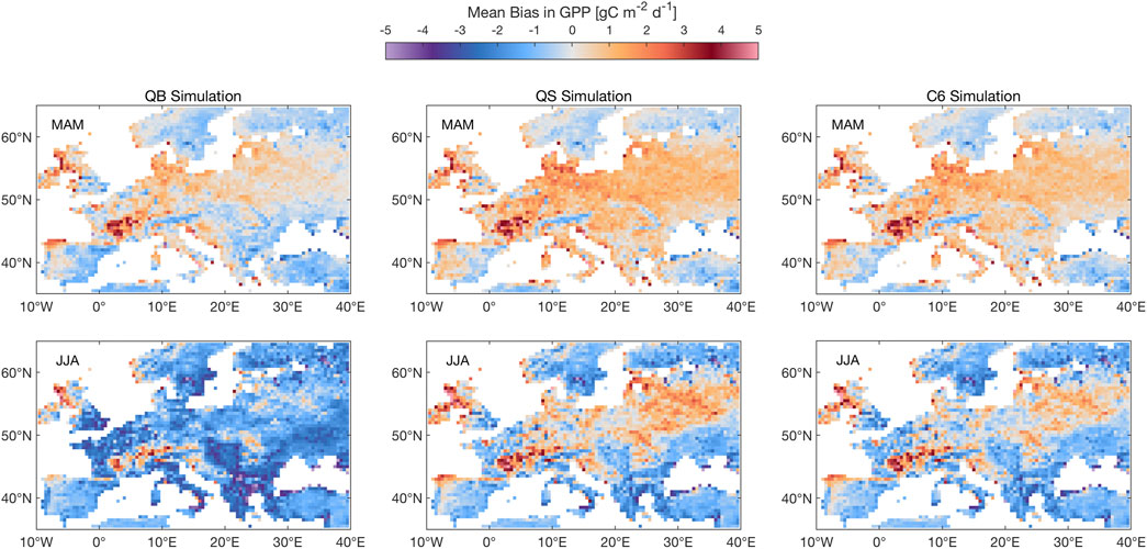
FIGURE 3. Mean climatological bias for GPP in simulations QB, QS and C6 against FLUXCOM observations. MAM mean (top row) and JJA mean (bottom row). Units: gC m⁻² d⁻¹.

Figure 4 shows the LE response, which, to a large extent, reflects the transpiration response, given the high vegetation fraction for these large-scale experiments. For the three models, QB, QS, and C6, latent heat tends to be overestimated in Spring nearly everywhere in Europe, while for Summer a dipole emerges, with a slight overestimation in North and Central Europe, but a pronounced underestimation in Southern Europe, very likely due to soil dessication. No significant differences are seen, however, between QB and C6 in any of the seasons, which is an important result in view of what has been found for the GPP response. Model QS shows some indication of a bias reduction in the NE portion of the domain, but a worsening in the SE (over Greece and Turkey).

FIGURE 4

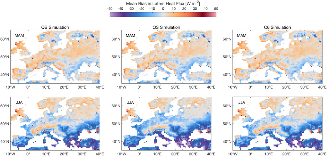
FIGURE 4. Same as Figure 3, albeit for latent heat. Units: W m⁻².

Figure 5 shows the sensible heat flux (SH) response, which is nearly insensitive to the model formulation in spring, and shows small regional responses in summer, which mirror the responses seen in the latent heat flux maps (Figure 4): this small response to model formulation is again rather expected (because the model was run with observed meteorology and is thus constrained) and rather reassuring, as in most years European plants are not water stressed for periods of time long enough to impact climate means.

FIGURE 5

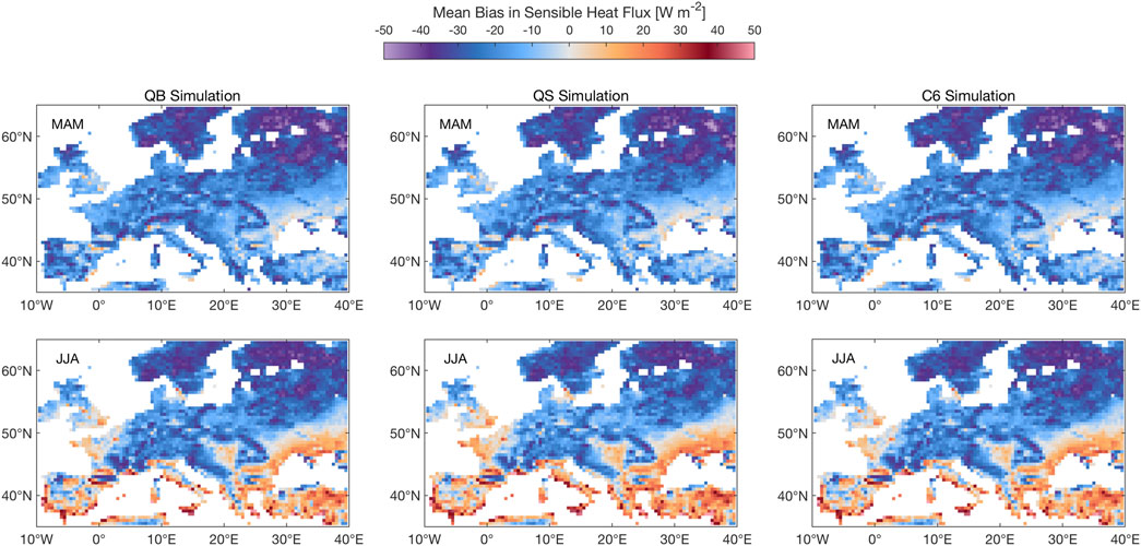
FIGURE 5. Same as Figure 3, albeit for sensible heat. Units: W m⁻².

Figure 6 shows the available soil moisture response in terms of the β factor in the soil: since it is a relative measure, and weighted by layer thickness, it reflects the effect on the bulk of the roots for the JULES vegetation (mostly forests and C3 grasses in this European domain), with a possible buffering effect from the deepest layer, which is more accessible to trees than grasses. The response of each model is quite strikingly different: while QB is virtually identical to CTL (some differences are expected, since these are long-term spun-up experiments, and any numerical residual would show strongly in a cumulative variable such as soil moisture), the QM response is mostly a strong drying, seen in all seasons, but with a strong North-West to South-East gradient. The response of QS is, instead, a moistening, again with a strong NW to SE gradient. The C6 response is, remarkably, nearly identical to the QB (CTL) response, indicating that this combined pathway for soil moisture impact on the surface latent heat flux is nearly soil moisture neutral. These responses are consistent with, and do help to interpret, the LE and SH responses seen previously in Figures 4, 5, both in terms of the N-S gradient and in terms of the seasonal evolution.

FIGURE 6

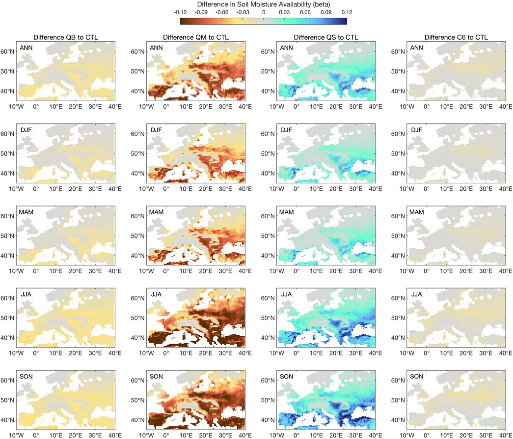
FIGURE 6. Climatology of available soil moisture, as indicated by ß in each simulation, as compared to the control simulation (CTL). All values apply to the full soil profile. ß is unitless.

Response to Multiple Droughts in the 1979–2011 Period

Figure 7 shows a panoramic view of all droughts in Europe, with different severities, both in terms of intensity (going as far as a Δβ exceeding −0.3) and of spatial extent. Key drought years present characteristics that are spatially consistent, indicative of a large-scale atmospheric forcing, and often corresponding to heat waves, such as 2003 and 2010, as discussed in Fischer et al. (2008) and in Russo et al. (2015). Notable droughts in recent times are 1995 (United Kingdom and Spain), 1996 (North Europe), 2002 (Poland, Belarus), 2003 and 2011, over most of Western Europe, 2005 (Spain) and 2010 (Russia, mostly outside the domain). By using the mask constructed from Figure 7, it is next possible to produce a synthesis plot that presents the response to the treatment of β, for each year in which a significant drought has been identified.

FIGURE 7

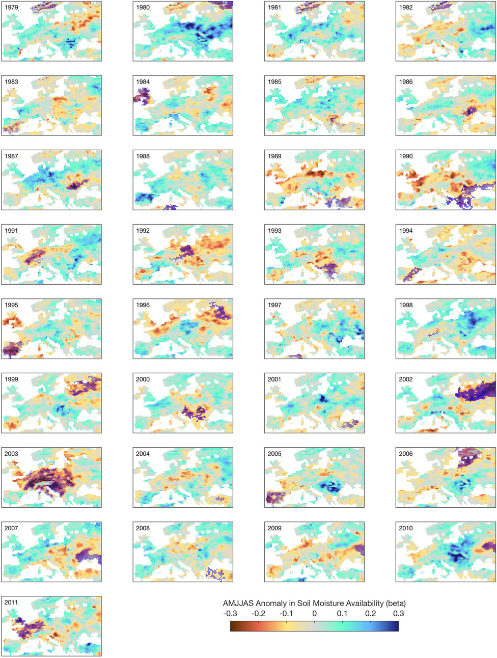
FIGURE 7. Annual extent and intensity of drought anomalies across Europe in the period 1979–2011, as revealed by the ß factor in the JULES land surface model (CTL experiment). ß is unitless.

Figure 8 provides a synthesis of model behavior for 20 soil moisture drought years, indicated by dots of different magnitude, according to spatial extent and intensity, expanding from the focus on the largest disturbance, 2003, which remains a prominent benchmark in terms of area extent and intensity. Figure 8 shows the summary of model flux errors, averaged over each drought year, extracted from the data used for Figures 3–5 (and defined as difference from identically processed FLUXCOM observations), against the annual AMMJAS Δβ.

FIGURE 8

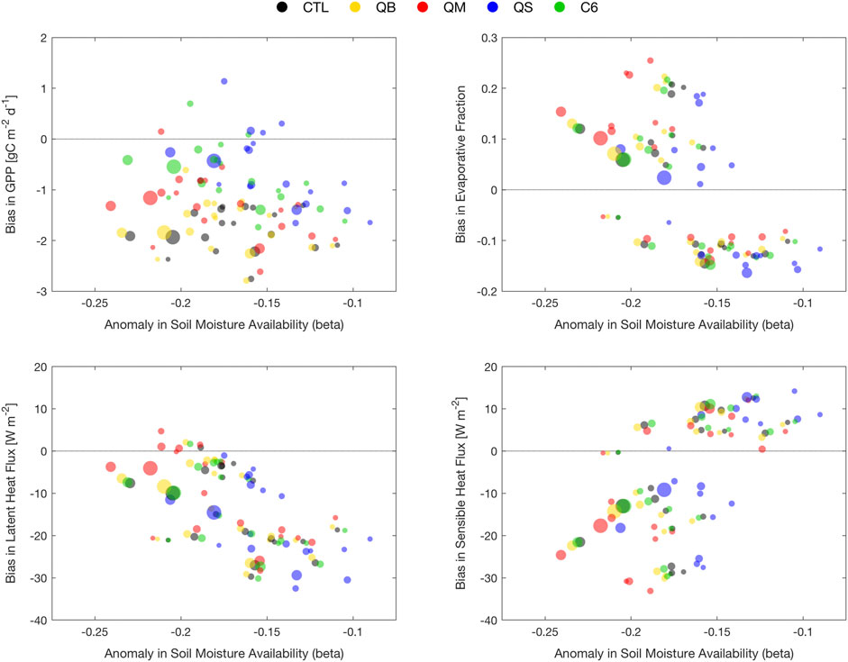
FIGURE 8. Model errors in GPP (top left), evaporative fraction (top right), latent heat (bottom left) and sensible heat (bottom right) for the top ten droughts in Europe in the period 1979–2011 identified via the mask developed from Figure 7.

Figure 8A shows that the majority of drought years correspond to years of (overly) depressed GPP; however, the depressed vegetation production response is strongly dependent on the treatment of $\beta$, which can be appreciated by how clustered the coloured dots are, and less dependent on the intensity of the drought, as the dots tend to be organized in horizontal bands, rather than on a diagonal. Simulations QS and C6 correspond to the data clusters with the least bias in GPP for those soil moisture drought years, independent of location.

Figure 8B shows the errors in the evaporative fraction (EF), which is included here to account for differences in the sum of SH and LE between simulations and FLUXCOM products. The errors are now aligned on a diagonal, with smaller values of Δβ mostly corresponding to a negative bias (caused by a positive error in SH and a negative error in LE, see Figure 8C, and Figure 8D), and larger values of Δβ leading to a positive bias in EF. Simulation QS is closest to EF observations for 2003, with C6 second-best, albeit similar to QB, and with QM displaying the largest bias. The small amplitude Δβ (negative EF bias) seem to correspond to points in the Northern portion of the domain.

For LE flux, Figure 8C shows that the error metric is now aligned on a diagonal (unlike GPP) and tends to be dominated by the southern portion of the domain, where JULES strongly underestimates LE in the climatology. As the drought severity increases, the LE flux bias is reduced, suggesting that the LE response to Δβ starts to plateau, and the model has an opportunity to “catch up” to observations. There are indications that QM, the most liberal treatment of β in terms of soil water usage, has the least error overall, while QS, the most conservative, is exaggerating the LE response, particularly at moderate Δβ levels. Relative advantages are not so clear for the other treatments (QB, C6), even for the largest events.

Figure 8D shows the error in SH as a function of Δβ, which is aligned on a diagonal with slope opposite to the one for LE: SH is strongly underestimated in severe drought cases, meaning that the observed heating from the anomalous 2003 soil dessication is not simulated faithfully, and slightly overestimated in moderate drought cases. For this variable, simulation QM seems to be slightly worse than the others for the most pronounced droughts (better skill for low intensity droughts), while QS seems to have a small advantage overall at medium Δβ levels; C6 is quite similar to QB in this respect.

The overall lesson is that, while GPP errors are affected systematically by the choice of β treatment, the errors in energy fluxes are shifted to different equilibria, reflecting climatological shifts in soil moisture, and could be interpreted as a near-neutral response.

Response to Extreme Atmospheric Forcing: The European Heat Wave of 2003

Figure 9 shows the evolution of GPP during the 2003 summer heat wave, as monthly means, from April to August, for simulations QB, QS, and C6, the most interesting ones, analyzed in terms of the evolution of model error (against FLUXCOM). While it is well-known that Spring 2003 saw clear skies and warmer conditions, leading to enhanced vegetation activity while there was still ample soil moisture availability, both QB and C6 exaggerate this response, particularly over France and Germany, with C6 showing the largest response in April, which implies a larger soil moisture usage. This deficit can then lead, via soil memory, to a suppressed GPP in each of the JJA months; in this respect, C6 is an improvement over QB, as it is apparently able to sustain a larger JJA GPP. Simulation QS is nearly identical to C6, albeit with a slightly smaller amplitude for the JJA signal for the Western Europe mean, therefore the smallest error overall, while simulation QM (not shown) has a far smaller response.

FIGURE 9

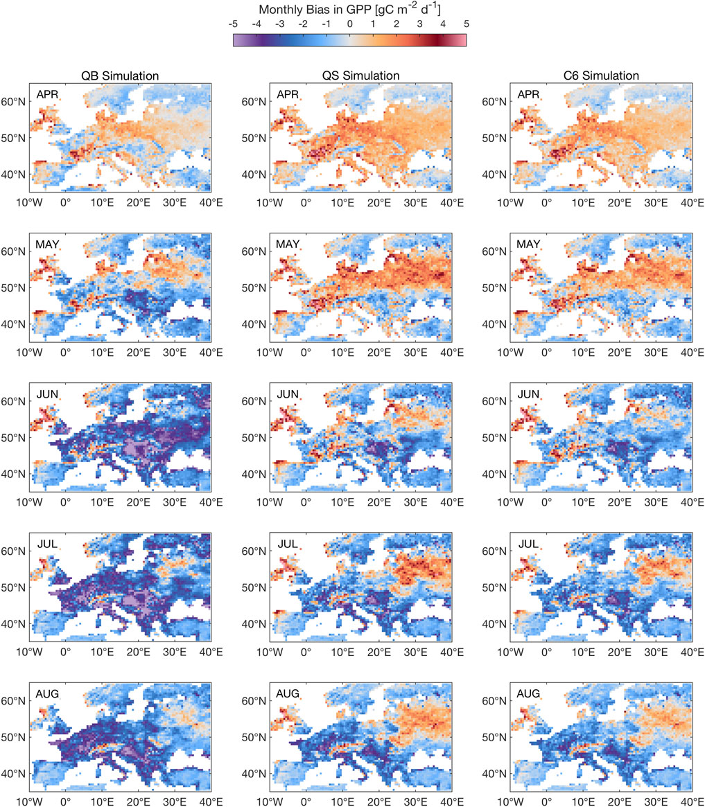
FIGURE 9. Seasonal evolution of GPP response to the 2003 heat wave for simulation QB, QS, C6, as compared to FLUXCOM. The 2003 season starts at the top row, with the April 2003 monthly mean response, and ends in August 2003, with the monthly mean response. Units: gC m⁻² d⁻¹.

For latent heat flux during the Summer 2003 heat wave (Figure 10), simulation C6 hardly shows any difference to CTL (better evidenced in the soil moisture maps, Figures 6, 11), while simulation QS displays a more interesting seasonal behavior, with a regional worsening of the dry bias in Spain and Eastern Europe (June), then in a region that covers France, Germany and Poland by August. This indicates that the enhanced GPP response in Spring has indeed consequences for the water cycle, via soil moisture memory, so that the errors in JJA are larger than for QB and C6. Simulation QM (not shown) shows a similar, albeit even more pronounced enhanced spring behavior, with a strong overestimation throughout, particularly from May to July, in most of central Europe, but then a relative reduction of the dry bias in August. These behaviors might amplify and lead to far worse summer conditions if the heat wave had been repeated in 2004 in this region.

FIGURE 10

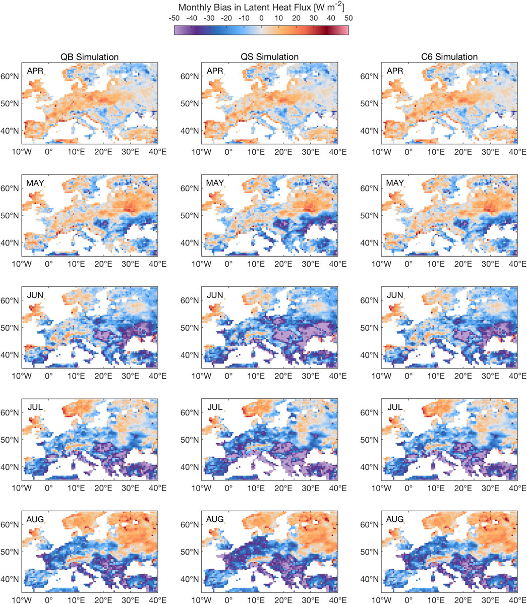
FIGURE 10. Seasonal evolution of Latent Heat Flux (LE) response to the 2003 heat wave for simulations QB, QS, C6 (as compared to FLUXCOM). The 2003 season starts at the top row, with the April 2003 monthly mean response, and ends in August 2003, with the monthly mean response. Units: W m⁻².

FIGURE 11

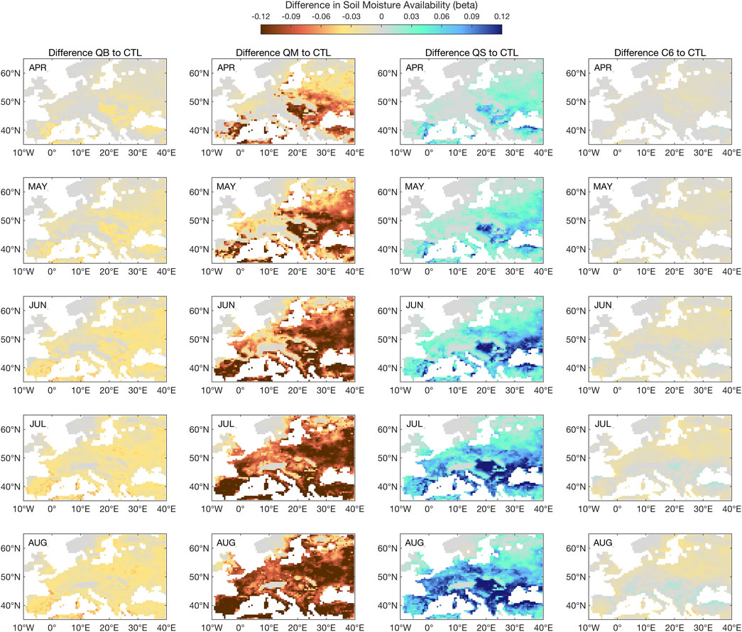
FIGURE 11. Seasonal evolution of available soil moisture response to the 2003 heat wave in all simulations, as compared to CTL. The 2003 season starts at the top row, with the April 2003 monthly mean response, and ends in August 2003, with the monthly mean response. ß is unitless.

Figure 11 reveals a soil moisture evolution for 2003 that mostly explains the above results for GPP and latent heat. Simulation QS is increasingly accumulating soil moisture in the soil, in a rather linear way, from April to August, but this is then reflected in too strong a limitation of transpiration, thus latent heat, as will be shown in Figure 12. Simulation C6 is closest to CTL, and demonstrates a neutral response to the soil moisture stress, despite having achieved the best performance in terms of the simulation of GPP in Figure 9. Simulation QM (not shown) responds as an enhanced QS: starting from already dry conditions, it develops a seasonally increasing drying in the soil, which is compatible with too liberal a use of soil moisture, e.g., for Eastern Europe in spring and summer.

FIGURE 12

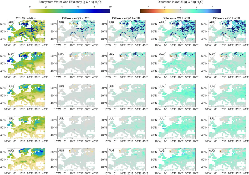
FIGURE 12. Seasonal evolution of ecosystem Water Use Efficiency (eWUE) for simulation CTL, followed by the difference between each simulation (QB, QS, C6), and CTL. Units are g C per kg of H₂0.

Comparison of Ecosystem Water Use Efficiency

Figure 12 shows a comparison of ecosystem water use efficiency (eWUE, calculated here from NPP and evapotranspiration at grid-box level) for the year 2003, one of the key years identified in Peters et al. (2018), as a seasonal evolution. It is clear that, as early as April, a large area of Europe experienced high eWUE, as the atmosphere was clear and net radiation abundant, but springtime soil moisture was already starting to become depressed, as was seen in Figure 11. As the season evolved, and assimilation (A) dropped due to increased plant water stress, particularly for the southern part of the domain, differences start to become obvious for the treatments involving a stomatal conductance route: QS and C6 show a clear advantage over the entire 45–60 latitude band, from May to August. This is quite easy to explain for simulation QS, which showed a large 2003 soil moisture surplus when compared to the other simulations, but more subtle for simulation C6, which shows virtually no change in soil moisture when compared to CTL, and even to QB. The C6 response must then be explained by changes in carbon assimilation, which must have become more efficient. It remains to be seen whether this advantage represents a realistic response, by further verification against observations.

The Diurnal and Seasonal Cycles of Stomatal Conductance

Figure 13 shows the diurnal and seasonal evolutions of stomatal conductance for water vapor (g_s) for a grid point in France nearest the location of maximum heating in summer 2003, and for the broadleaf land tile (the C3 grass response is very similar, albeit less sharp). Time runs from 2002, near the bottom, to 2006 near the top of each panel: 2002 was a relatively cold and wet summer in this region, while 2003 experienced one of the worst summer heat waves in recent times for this portion of Europe. By comparing the different responses, from left to right, pathway QB sees a strong reduction in stomatal conductance in 2003, as compared to 2002 and later years, in which a vegetation recovery occurred. An even stronger response can be seen in the second column, corresponding to pathway QS, which is easy to understand from the point of view of the $\beta$ (Eq. 4). The mesophyll pathway (QM) shows the least reduction of stomatal conduction in 2003, while C6 exhibits an interim response in comparison to QB and QM.

FIGURE 13

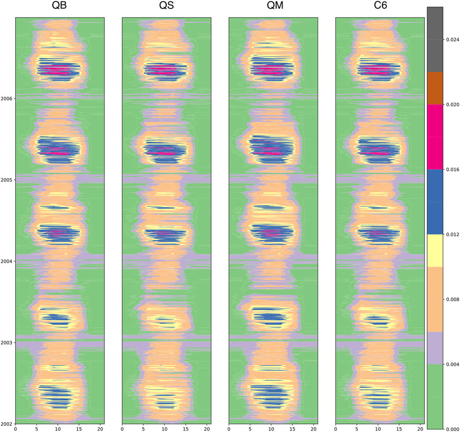
FIGURE 13. The diurnal and seasonal evolution of stomatal conductance (g_s, m s⁻¹) as filled contours for the JULES Plant Functional Type 1 (Broadleaf Trees) at a grid point in France. The diurnal cycle (GMT hour) is shown on the x axis, while the seasonal cycle (indicated by years from 2002 to 2006, top) is shown on the y axis. The four experiments are QB, QS, QM, and C6 in each column.

The Diurnal and Seasonal Cycles of $C_i\left(\chi \right)$

Figure 14 shows the diurnal and seasonal evolution of C_i for the same grid point shown in Figure 12, which is fully indicative of $\chi$ evolution, since reference level CO₂ is prescribed in these simulations, due to the atmosphere being forced. The difference between the four different simulations is striking, particularly for years in which plants experienced strong environmental stress, such as 2003. Simulation QS exhibits the strongest response: by closing the stomata during periods of increased drying, such as early 2003, the C_i level drops dramatically, as had been anticipated in Figure 2. However, at the peak of the 2003 summer heat wave, during the late stage of the diurnal cycle, when the soil moisture stress (and the mounting temperature stress, which compounds the effect) starts to reach its peak, C_i returns towards the C_a value (in the early morning and late evening), because photosynthesis stops, also as seen previously in Figure 2, due to a compound stress effect. Simulation C6 shows a response that is qualitatively similar, albeit with smaller magnitude, while simulations QB and QM hardly drop the C_i level at all, also consistent with what had been seen in Figure 2.

FIGURE 14

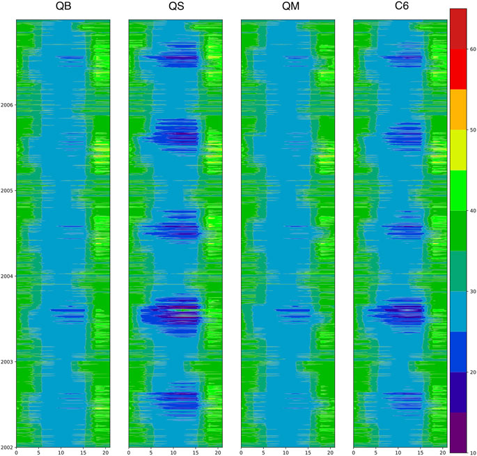
FIGURE 14. The diurnal and seasonal evolution of internal CO₂ pressure (C_i, Pa) as filled contours for the JULES Plant Functional Type 1 (Broadleaf Trees) at a grid point in France. The diurnal cycle (GMT hour) is shown on the x axis, while the seasonal cycle (indicated by years from 2002 to 2006, top) is shown on the y axis. The four experiments are QB, QS, QM, and C6 in each column.

Comparison With Intrinsic Water Use Efficiency From FLUXNET Observations

It is expected that in years of drought vegetation stress will also be revealed by measurements of isotopic discrminination, which was the main topic of Peters et al. (2018). The mechanisms involved in the process of photosynthesis favor the lighter ¹²CO₂ molecule over the heavier ¹³CO₂ molecule, at several stages in the mechanistic chain. This leads to ‘discrimination’: stressed vegetation will present lower δ¹³C = ¹³C/¹²C values, relative to the atmosphere, and the difference is denoted by the symbol Δ = δ¹³C_a−δ¹³C_v (units of ‰). In JULES, Δ can be estimated approximately, by using in Eq. 6, Methods. Supplementary Figure S1 shows the domain average behavior of the four C3 vegetation types in the JULES experiments, as annual anomalies for the year 2003. Because of drought stress, it is expected that NPP will be reduced compared to other years, and that Δ will be smaller, which is: see Figure S1 of Peters et al. for the curve of C_i/C_a vs Δ, what is shown by observations and by the model intercomparison in Peters et al. (2018). Supplementary Figure S1 reveals that grasses suffer the most during the severe drought year of 2003, with NPP reductions of over 100 Tg C, while needleleaf trees are quite resilient (also because they are mostly located outside the area of drought, but a similar calculation with a drought mask shows the same qualitative behavior). Simulation C6 shows the least drop in NPP and the most realistic response in terms of the combined NPP/Δ metric, as compared to the data in Peters et al. (2018), with the anomaly in Δ reaching values of -0.15 for grasses, while simulation QB tends to have a Δ closer to 0 or above. It is next possible to plot the combined gridbox Δ data on a map and to compare with observations.

Figure 15 shows a superposition of iWUE in observations (Peters et al., 2018), and as produced by JULES, computed by using Eq. 7, and using 3-hourly C_i at PFT level. The four panels show the response (marked by dots and color-coded for change in iWUE, as originally presented in Peters et al., 2018) over the region mostly affected by the 2003 heat wave, namely Western Europe, where iWUE reached a maximum, indicated by the green color. The dots show data from point observations; the insets at the top right of each panel show the PDF of values in the domain. It is clear from the comparison of the four panels that the biochemical pathway for β fails to simulate the high level of iWUE reached by plants in Western Europe during the 2003 heat wave. The β pathways that retain some level of control via stomatal conductance are more realistic, with the C6 (combined) pathway achieving the best match with observations, as had shown by other case studies in Southern Spain (see E11).

FIGURE 15

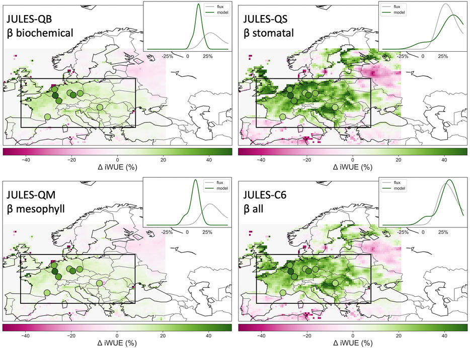
FIGURE 15. Water Use Efficiency anomaly for 2003 (Δ iWUE, %), as revealed by the Peters et al. (2018) dataset and as simulated by JULES using the four different ß pathways.

The original multi-model presentation of this figure (see Supplementary Material in Peters et al., 2018), indicated that most LSMs struggle to simulate the shift to higher iWUE (greener colors), which is summarized for the observation sites in the PDFs in each inset. The original JULES-CTL had in fact failed to capture both the magnitude and spatial extent of the impact, similar to the QB simulation developed for this study, which clearly missed the high level of iWUE reached by plants in Western Europe during the 2003 heat wave, so that it was replaced with configuration C6.

iWUE and eWUE originate at different scales in the model, the first stomatal, via the C_i route, and the second involving area averaging of carbon and water fluxes over each grid box, weighted by PFT abundance, and are thus compared against different types of observations. The consistency of the improvement, from iWUE to eWUE, over a coarser scale and over a larger domain, for well-observed events like 2003, gives us further confidence that our proposed pathways strongly improve the JULES drought response, not just for reductions in GPP and LE (achieved in all schemes) but especially for their relative ratio (captured best by the C6 configuration).

Discussion

The E11 model was implemented in a state-of-the-art LSM, JULES, now with complete freedom in enabling soil moisture stress to limit photosynthesis (QB), stomatal conductance (QS) or mesophyll conductance (QM), independent of any a-priori assumptions on what are the controlling mechanisms and pathways. A combined treatment (C6) was also tested, taken from the E11 recommendations. A conscious decision was made, at this stage, to choose a framework in which GCM biases in surface energy balance would not cloud the investigation, thus observed meteorology was used as a forcing. Additionally, the parsimonious requirements for computational resources enabled a broad set of experiments, including a lengthy LSM spin-up (cycles up to 300 years) for each, could be made feasible, unlike in a full GCM set-up. It has also to be remembered that, at this stage, the solution algorithm has yet to be made efficient, and these simulations, based on polynomial solutions, are slow, unsuitable for a GCM environment.

The primary purpose of this LSM development was indeed to answer the question of whether or not the a-priori decision of implementing the β limitation on just one of the model components, e.g., photosynthesis, as in models based on the Collatz et al. (1991) formulation, has consequences for our ability to credibly predict the future of land surface dynamics. There is strong demand for predicting the fate of feedbacks between the energy and water cycles (but including carbon over longer periods), as triggered by soil moisture deficits, but such an investigation must be carried out incrementally, with many of the feedbacks purposefully disabled, in order to enable clearer understanding.

The overall model sensitivity seems to be revealed more systematically on the GPP side than on the energy fluxes, as adjustments occur, as revealed by EF, also in response to long-term soil moisture memory. This flux adjustment can be seen as a reassuring result in this particularly constrained experimental setup. Because of non-linearities in the system, models in which $\beta$ is applied to stomatal conductance tend to limit transpiration, thus to conserve soil moisture, while only partially affecting GPP, except perhaps in parts of Southern Europe at the end of summer. Models in which $\beta$ is applied to mesophyll conductance tend to overuse soil moisture, creating a deficit, particularly evident in semi-arid regions, and causing stress (from drought and heating) at the end of summer, but this does not seem to have any effect on GPP, implying that water use efficiency is increased in Southern Europe.

Analysis focusing on the 2003 summer heat wave revealed that the environmental stress, as an earlier and more intensive use of soil moisture by evaporation across Europe, causes an even stronger sensitivity response in the four models that have been analyzed. While a negative bias in GPP is present in all models, the 2003 heat wave is most credibly simulated by applying the combined pathway (C6) for the months June, July and August, despite an earlier overestimation of GPP. The heat wave can, however, develop more severely (making the dry bias even worse) when using models with $\beta$ applied directly to stomatal control, particularly in Southern Europe, or be classified as less severe when using any models that involve mesophyll conductance (e.g., QM, or even the more moderate C6). It is unclear whether the more intensive water use incurred by models including the mesophyll pathway would be sustainable if the anomalously dry and warm conditions were to last for more than 1 year, unlike what happened in post-2003: for Europe winter precipitation is normally sufficient to recharge soil moisture on an interannual basis, but this is not true for other regions, e.g. for the Southern United States, which has been experiencing multi-year drought conditions in recent years.

For $\chi$, the diurnal and seasonal behavior uncovered in the latter part of the study are fully consistent with the expectations raised by the idealized study in the introduction: during the heat wave, enhanced stress conditions (e.g., at noon and/or at the peak of summer) result in stomatal closure, which then results in a strong reduction of $\chi$, but does not necessarily need imply a direct reduction of GPP, as caused instead by making the decisions, conscious or not, of imposing $\beta$ on carbon assimilation, as is done in many second-generation LSMs. Comparisons provided in E11, and many references therein, indicate that low levels of $\chi$, made possible in JULES with the new generalized analytical scheme, are credible, and indicative of a correct chain of mechanisms.

A strong confirmation of this interpretation is the fact that results of all experiments were now used to compute iWUE from C_i, and showed that the C6 formulation performs comparatively better against the data collected and analysed in Peters et al. (2018) study, revealing a very realistic response of the model to the 2003 perturbation, which seems governed by mechanisms at the stomatal level, and primarily by the fast evolution of C_i. The comparison of eWUE (performed on grid-scale variables) and iWUE (performed at stomatal and PFT level C_i every 3 h) show complete consistency and indicates that applying the $\beta$ stress to photosynthesis alone is unable to reproduce a credible vegetation response to the large 2003 event, as well as, from the new analysis in this study, to the other European droughts in the simulated period.

It has also to be remembered that C_i can also be used to compute the isotopic discrimination metric, Δ, and that in the Peters et al. (2018) study JULES (in the C6 configuration) performed best when assessed against independent isotopic measurements, and against other models, some of which had been specifically developed to simulate isotopic discrimination. This further confirmation (and more analysis, see Supplementary Material), via the C_i chain of mechanisms, indicates that C_i dynamics is more credibly represented by allowing soil moisture stress to affect all plant function at once, which has important implications for applications to studies of climate variability and change including the carbon cycle.

There are, however, shortcomings in the adopted methodology: it is impossible, with the current set of experiments, driven by observed meteorology, to estimate the full impact of the surface temperature feedback, because the experimental setup only allows feedback to the leaf-level temperature, but this is then nudged towards the value of the atmospheric near-surface temperature, for each JULES model time step in the 3-hourly meteorological forcing data intervals. If anything, because of the use of observed meteorology as drivers, the present results are indicative of a muted version of possible land-atmosphere feedbacks that can be unleashed by choosing one model configuration over another.

The impact of feedbacks would very likely be significantly larger in a free-running GCM experiment. This may result in more dramatic conclusions with respect to suitability for the CMIP-type climate predictions, particularly if any form of dynamic vegetation (e.g., dynamic phenology or phenology plus competition) is taken into account, as the present results indicate that soil moisture response is over large scales and long time periods, thus with the potential for altering important components of the terrestrial carbon cycle.

However, while the experiments in this study have demonstrated that the generalized $\beta$ scheme is fully functional (and numerically stable), the solution scheme is more expensive (at least a factor 3x) than the original JULES scheme, because of the use of complex polynomials (see Supplementary Material), which are onerous and hard to optimize, even with modern compilers.

A Practical Proposal for Future Solution Schemes for the E11 Model

As discussed above, the new implementation of the E11 model, now inside a state-of-the-art land surface scheme, JULES, was successful, and the prognostics that are produced seem sound in all respects. The scheme is, however, more expensive than the original (iterative) scheme in JULES; this is currently untenable for use in GCMs, but this study suggests that the same set of experiments should now be run in a full GCM setting. In order to find viable configurations, Supplementary Figure S2 in Supplementary Materials suggests possible future avenues for a more computationally parsimonious implementation. Starting from the top, the standard JULES scheme is summarized, then the E11 scheme implemented in this paper. Two further solution schemes are proposed. The first one is inspired by a classic forward-backward in time (FTBT) scheme, used in a variety of ocean and atmospheric models (e.g. in WRF), either A or g_s are diagnosed at the start of each time step, and then a quadratic equation for C_c is solved at each time step (depending on g_s or A on alternate time steps), which is cheaper than solving a cubic equation. A second additional scheme is proposed, in which g_s is initially estimated as a simple prognostic (as in Sellers et al., 1996, but also reminiscent of the modified Matsuno, 1966, scheme, in which an initial Euler step precedes an imitation of an implicit time scheme), leading again to a quadratic equation for the other two variables. This implementation was successful in SiB2 and also reduced fast time oscillations, which can potentially be incurred by FTBT-type schemes. This same approach could in the future be applied to the prediction of χ, or to C_c.

Once a suitable numerical implementation is found, with computational costs comparable to the standard JULES scheme, and once a C4 scheme for the $\beta$ pathway is developed, it will be possible to run the same type of experiment in the HadGEM3-GC31 GCM, albeit only for the most promising configuration, C6, given the large computational costs involved.

Summary and Conclusion

We have implemented the generalized, analytical and simultaneous soil water stress scheme of Egea et al. (2011) into a state-of-the-art land surface model, JULES, which can be used at multiple scales, including global offline and coupled to the HadGEM3 GCM. In this study, we have chosen to focus on the European region, and to drive JULES with observed meteorology, in order to retain a degree of control on feedbacks and to enable comparison with the standard (CTL) JULES configuration. The implementation required the development of a new solution set for the three simultaneous equations that are used to prognose A, g_s, and C_c. A further development in Egea et al. (2011) that was implemented in JULES is the inclusion of mesophyll conductance. The new prognostic scheme was shown to be successful and to enable complete freedom in imposing soil water stress, $\beta ,$via any pathways (stomatal, biochemical, mesophyll) or any combinations thereof, including non-linear relationships between soil moisture values and $\beta$.

Results show that the treatment of soil moisture stress matters to the simulation of land surface climate in Europe, particularly for summer, but even extending into Spring and Autumn. All land surface prognostics are affected by the choice of $\beta$ pathway, but particularly those controlling water and carbon fluxes between the land and the atmosphere, as well as soil moisture dynamics, which shows a cumulative effect, with strong depletion if a mesophyll conductance pathway is chosen, and strong surplus (particularly in the Southern part of the domain) if a stomatal pathway is chosen. Seasonal and climatological feedbacks between soil moisture levels and land surface fluxes are then triggered.

Responses to the drought involved in the exceptional 2003 summer heat wave, also expanded to other droughts in the last 30 years, demonstrate how important vegetation function feedbacks, from intra-seasonal to interannual, can be initiated even in a modelling framework in which the atmospheric signal is imposed. Under such conditions, it has been shown that models including a stomatal pathway can reach very low levels of stomatal conductance, accompanied by very low, and realistic, $\chi$ levels, which result in more realistic simulation of intrinsic and ecosystem Water Use Efficiency, as well as, via a specific metric of isotopic fractionation (Δ), large scale anomalies in vegetation activity. This skill in representing the chain of mechanisms involved in drought response is not normally seen in LSMs, suggesting that the realistic prediction of the feedbacks involved in changes in the carbon cycle requires re-visiting some of the most fundamental assumptions in LSMs used for climate prediction.

Data Availability Statement

The raw data supporting the conclusions of this article will be made available by the authors, without undue reservation.

Author Contributions

PV, GE and AV designed the experiments. GE and PV implemented the E11 model into JULES, which required the development of new numerical solution methods (see Supplementary Materials), mostly accomplished by GE. PV and BB-S ran all experiments with JULES 2.2; PV then re-ported the E11 model to the more recent JULES 4.4 and ran initial quality assurance and stability experiments, but PM finally completed the full set of experiments presented in this article. MT and OM performed the analysis of climatological biases and variability; MT produced the analysis of drought years and the synthesis of annual GPP responses, as well as revised energy flux figures. PV conducted the idealised WUE and $\chi$ analyses at the start of the article and wrote the diagnostic code for C_i, VPD and T* at stomatal and PFT levels. WP helped with the water-use efficiency analysis and provided comments on the text.

Funding

This research has been supported by the Horizon 2020 programme: PRIMAVERA (grant no. 641727), the National Environmental Research Council (NERC), United Kingdom Earth System Modelling (grant no. NE/N017951/1) and by NERC grant IMPETUS (NE/L010488/1). WP acknowledges funding from the H2020 ERC project ASICA (grant no. 649087).

Conflict of Interest

The authors declare that the research was conducted in the absence of any commercial or financial relationships that could be construed as a potential conflict of interest.

Publisher’s Note

All claims expressed in this article are solely those of the authors and do not necessarily represent those of their affiliated organizations, or those of the publisher, the editors and the reviewers. Any product that may be evaluated in this article, or claim that may be made by its manufacturer, is not guaranteed or endorsed by the publisher.

Acknowledgments

PLV and PM acknowledge the NERC-Met Office HRCM research programme and the EU-Horizon2020 PRIMAVERA programme. MT and PM acknowledge the CSSP Porcelain grant. GE acknowledges the award of a postdoctoral fellowship from Fundación Ramón Areces (Madrid, Spain) and support from the University of Seville. We kindly acknowledge the contributions from Mr E. van Schaik to the research presented. This work used eddy covariance data acquired by the FLUXNET community. We acknowledge the financial support to the eddy covariance data harmonization provided by CarboEuropeIP, FAO-GTOS-TCO, iLEAPS, Max Planck Institute for Biogeochemistry, National Science Foundation, University of Tuscia, Université Laval and Environment Canada, and US Department of Energy and the database development and technical support from Berkeley Water Center, Lawrence Berkeley National Laboratory, Microsoft Research eScience, Oak Ridge National Laboratory, University of California Berkeley, University of Virginia.

Supplementary Material

The Supplementary Material for this article can be found online at: https://www.frontiersin.org/articles/10.3389/fenvs.2021.689301/full#supplementary-material

References

Anderegg, W. R. L., and Venturas, M. D. (2020). Plant Hydraulics Play a Critical Role in Earth System Fluxes. New Phytol. 226, 1535–1538. doi:10.1111/nph.16548

PubMed Abstract | CrossRef Full Text | Google Scholar

Baldocchi, D. (1994). An Analytical Solution for Coupled Leaf Photosynthesis and Stomatal Conductance Models. Tree Physiol. 14, 1069–1079. doi:10.1093/treephys/14.7-8-9.1069

PubMed Abstract | CrossRef Full Text | Google Scholar

Ball, J. T., Woodrow, I. E., and Berry, J. A. (1987). “A Model Predicting Stomatal Conductance and its Contribution to the Control of Photosynthesis under Different Environmental Conditions,” in Progress in Photosynthesis Research. Editor J. Biggens (Dordrecht: Martinus Nijhoff), IV, 221–224. doi:10.1007/978-94-017-0519-6_48

CrossRef Full Text | Google Scholar

Beer, C., Reichstein, M., Tomelleri, E., Ciais, P., Jung, M., Carvalhais, N., et al. (2010). Terrestrial Gross Carbon Dioxide Uptake: Global Distribution and Covariation with Climate. Science 329, 834–838. doi:10.1126/science.1184984

PubMed Abstract | CrossRef Full Text | Google Scholar

Berg, A., Findell, K., Lintner, B., Giannini, A., Seneviratne, S. I., van den Hurk, B., et al. (2016). Land-atmosphere Feedbacks Amplify Aridity Increase over Land under Global Warming. Nat. Clim Change 6, 869–874. doi:10.1038/nclimate3029

CrossRef Full Text | Google Scholar

Best, M. J., Pryor, M., Clark, D. B., Rooney, G. G., Essery, R. L. H., Ménard, C. B., et al. (2011). The Joint UK Land Environment Simulator (JULES), Model Description - Part 1: Energy and Water Fluxes. Geosci. Model. Dev. Discuss. 4, 595–640. doi:10.5194/gmdd-4-595-2011

CrossRef Full Text | Google Scholar

Clark, D. B., Mercado, L. M., Sitch, S., Jones, C. D., Gedney, N., Best, M. J., et al. (2011). The Joint UK Land Environment Simulator (JULES), Model Description - Part 2: Carbon Fluxes and Vegetation Dynamics. Geosci. Model. Dev. 4, 701–722. doi:10.5194/gmd-4-701-2011

CrossRef Full Text | Google Scholar

Collatz, G. J., Ball, J. T., Grivet, C., and Berry, J. A. (1991). Physiological and Environmental Regulation of Stomatal Conductance, Photosynthesis and Transpiration: a Model that Includes a Laminar Boundary Layer. Agric. For. Meteorol. 54, 107–136. doi:10.1016/0168-1923(91)90002-8

CrossRef Full Text | Google Scholar

Collatz, G., Ribas-Carbo, M., and Berry, J. (1992). Coupled Photosynthesis-Stomatal Conductance Model for Leaves of C4 Plants. Funct. Plant Biol. 19, 519–538. doi:10.1071/pp9920519

CrossRef Full Text | Google Scholar

Cox, P. M., Huntingford, C., and Harding, R. J. (1998). A Canopy Conductance and Photosynthesis Model for Use in a GCM Land Surface Scheme. J. Hydrol. 212-213, 79–94. doi:10.1016/S0022-1694(98)00203-0

CrossRef Full Text | Google Scholar

De Kauwe, M. G., Medlyn, B. E., Walker, A. P., Zaehle, S., Asao, S., Guenet, B., et al. (2017). Challenging Terrestrial Biosphere Models with Data from the Long-Term Multifactor Prairie Heating and CO 2 Enrichment experiment. Glob. Change Biol. 23, 3623–3645. doi:10.1111/gcb.13643

PubMed Abstract | CrossRef Full Text | Google Scholar

Dewar, R., Mauranen, A., Mäkelä, A., Hölttä, T., Medlyn, B., and Vesala, T. (2018). New Insights into the Covariation of Stomatal, Mesophyll and Hydraulic Conductances from Optimization Models Incorporating Nonstomatal Limitations to Photosynthesis. New Phytol. 217, 571–585. doi:10.1111/nph.14848

PubMed Abstract | CrossRef Full Text | Google Scholar

Egea, G., Verhoef, A., and Vidale, P. L. (2011). Towards an Improved and More Flexible Representation of Water Stress in Coupled Photosynthesis-Stomatal Conductance Models. Agric. For. Meteorol. 151 (10), 1370–1384. doi:10.1016/j.agrformet.2011.05.019

CrossRef Full Text | Google Scholar

Eller, C. B., Rowland, L., Mencuccini, M., Rosas, T., Williams, K., Harper, A., et al. (2020). Stomatal Optimization Based on Xylem Hydraulics (SOX) Improves Land Surface Model Simulation of Vegetation Responses to Climate. New Phytol. 226, 1622–1637. doi:10.1111/nph.16419

PubMed Abstract | CrossRef Full Text | Google Scholar

Essery, R., Pomeroy, J., Parviainen, J., and Storck, P. (2003). Sublimation of Snow from Coniferous Forests in a Climate Model. J. Clim. 16 (11), 1855–1864. doi:10.1175/1520-0442(2003)016<1855:sosfcf>2.0.co;2

CrossRef Full Text | Google Scholar

Farquhar, G. D., von Caemmerer, S., and Berry, J. A. (1980). A Biochemical Model of Photosynthetic CO2 Assimilation in Leaves of C3 Species. Planta 149, 78–90. doi:10.1007/bf00386231

PubMed Abstract | CrossRef Full Text | Google Scholar

Farquhar, G., and Wong, S. (1984). An Empirical Model of Stomatal Conductance. Funct. Plant Biol. 11, 191–209. doi:10.1071/pp9840191

CrossRef Full Text | Google Scholar

Gerten, D., Schaphoff, S., Haberlandt, U., Lucht, W., and Sitch, S. (2004). Terrestrial Vegetation and Water Balance-Hydrological Evaluation of a Dynamic Global Vegetation Model. J. Hydrol. 286, 249–270. doi:10.1016/j.jhydrol.2003.09.029

CrossRef Full Text | Google Scholar

Guimberteau, M., Zhu, D., Maignan, F., Huang, Y., Yue, C., Dantec-Nédélec, S., et al. (2018). ORCHIDEE-MICT (v8.4.1), a Land Surface Model for the High Latitudes: Model Description and Validation. Geosci. Model. Dev. 11, 121–163. doi:10.5194/gmd-11-121-2018

CrossRef Full Text | Google Scholar

Harper, A. B., Williams, K. E., McGuire, P. C., Duran Rojas, M. C., Hemming, D., Verhoef, A., et al. (2021). Improvement of Modelling Plant Responses to Low Soil Moisture in JULESvn4.9 and Evaluation against Flux tower Measurements. Geosci. Model. Dev. 14 (6), 3269–3294. doi:10.5194/gmd-2020-273

CrossRef Full Text | Google Scholar

Haynes, K. D., Baker, I. T., Denning, A. S., Stöckli, R., Schaefer, K., Lokupitiya, E. Y., et al. (2019). Representing Grasslands Using Dynamic Prognostic Phenology Based on Biological Growth Stages: 1. Implementation in the Simple Biosphere Model (SiB4). J. Adv. Model. Earth Syst. 11 (12), 4423–4439. doi:10.1029/2018ms001540

CrossRef Full Text | Google Scholar

Jacobs, C. M. J., Van den Hurk, B. M. M., and de Bruin, H. A. R. (1996). Stomatal Behaviour and Photosynthetic Rate of Unstressed Grapevines in Semi-arid Conditions. Agric. For. Meteorol. 80, 111–134. doi:10.1016/0168-1923(95)02295-3

CrossRef Full Text | Google Scholar

Jung, M., Koirala, S., Weber, U., Ichii, K., Gans, F., Camps-Valls, G., et al. (2019). The FLUXCOM Ensemble of Global Land-Atmosphere Energy Fluxes. Sci. Data 6, 74. doi:10.1038/s41597-019-0076-8

PubMed Abstract | CrossRef Full Text | Google Scholar

Liang, X., Lettenmaier, D. P., Wood, E. F., and Burges, S. J. (1994). A Simple Hydrologically Based Model of Land Surface Water and Energy Fluxes for General Circulation Models. J. Geophys. Res. 99 (D7), 14415–14428. doi:10.1029/94JD00483

CrossRef Full Text | Google Scholar

Mäkelä, J., Knauer, J., Aurela, M., Black, A., Heimann, M., Kobayashi, H., et al. (2019). Parameter Calibration and Stomatal Conductance Formulation Comparison for Boreal Forests with Adaptive Population Importance Sampler in the Land Surface Model JSBACH. Geosci. Model. Dev. 12 (9), 4075–4098. doi:10.5194/gmd-12-4075-2019

CrossRef Full Text | Google Scholar

Matsuno, T. (1966). Numerical Integrations of the Primitive Equations by a Simulated Backward Difference Method. J. Meteorol. Soc. Jpn. 44, 76–84. doi:10.2151/jmsj1965.44.1_76

CrossRef Full Text | Google Scholar

Medlyn, B. E., De Kauwe, M. G., Zaehle, S., Walker, A. P., Duursma, R. A., Luus, K., et al. (2016). Using Models to Guide Field Experiments: A Priori Predictions for the CO 2 Response of a Nutrient and Water-Limited Native Eucalypt woodland. Glob. Change Biol. 22, 2834–2851. doi:10.1111/gcb.13268

PubMed Abstract | CrossRef Full Text | Google Scholar

Nemani, R. R., Keeling, C. D., Hashimoto, H., Jolly, W. M., Piper, S. C., Tucker, C. J., et al. (2003). Climate-Driven Increases in Global Terrestrial Net Primary Production from 1982 to 1999. Science 300, 1560–1563. doi:10.1126/science.1082750

PubMed Abstract | CrossRef Full Text | Google Scholar

Niu, G. Y., Fang, Y. H., Chang, L. L., Jin, J., Yuan, H., and Zeng, X. (2020). Enhancing the Noah-MP Ecosystem Response to Droughts with an Explicit Representation of Plant Water Storage Supplied by Dynamic Root Water Uptake. J. Adv. Model. Earth Syst. 12 (11), e2020MS002062. doi:10.1029/2020ms002062

CrossRef Full Text | Google Scholar

Oleson, K., Lawrence, D. M., Bonan, G. B., Drewniak, B., Huang, M., Koven, C. D., et al. (2013). Technical Description of Version 4.5 of the Community Land Model (CLM), NCAR Earth System Laboratory – Climate and Global Dynamics Division. Technical Report. Boulder, Colorado, USA. TN-503+STR.

Google Scholar

Paschalis, A., Fatichi, S., Zscheischler, J., Ciais, P., Bahn, M., Boysen, L., et al. (2020). Rainfall Manipulation Experiments as Simulated by Terrestrial Biosphere Models: Where Do We Stand? Glob. Change Biol. 26, 3336–3355. doi:10.1111/gcb.15024

PubMed Abstract | CrossRef Full Text | Google Scholar

Peters, W., van der Velde, I. R., van Schaik, E., Miller, J. B., Ciais, P., Duarte, H. F., et al. (2018). Increased Water-Use Efficiency and Reduced CO2 Uptake by Plants during Droughts at a continental Scale. Nat. Geosci. 11, 744–748. doi:10.1038/s41561-018-0212-7

PubMed Abstract | CrossRef Full Text | Google Scholar

Powell, T. L., Galbraith, D. R., Christoffersen, B. O., Harper, A., Imbuzeiro, H. M. A., Rowland, L., et al. (2013). Confronting Model Predictions of Carbon Fluxes with Measurements of Amazon Forests Subjected to Experimental Drought. New Phytol. 200, 350–365. doi:10.1111/nph.12390

PubMed Abstract | CrossRef Full Text | Google Scholar

Prentice, I. C., Dong, N., Gleason, S. M., Maire, V., and Wright, I. J. (2014). Balancing the Costs of Carbon Gain and Water Transport: Testing a New Theoretical Framework for Plant Functional Ecology. Ecol. Lett. 17, 82–91. doi:10.1111/ele.12211

PubMed Abstract | CrossRef Full Text | Google Scholar

Press, W. H., Flannery, B. P., Teukolsky, S. A., and Vetterling, W. T. (1989). Numerical Recipes: The Art of Scientific Computing. Cambridge, U.K.: Cambridge University Press, 992.

R Development Core Team (2010). R: A Language and Environment for Statistical Computing. Vienna, Austria: R Foundation for Statistical Computing. Available at: http://www.R-project.org (ISBN 3-900051-07-0.

Restrepo-Coupe, N., Levine, N. M., Christoffersen, B. O., Albert, L. P., Wu, J., Costa, M. H., et al. (2017). Do dynamic Global Vegetation Models Capture the Seasonality of Carbon Fluxes in the Amazon basin? A Data-Model Intercomparison. Glob. Change Biol. 23, 191–208. doi:10.1111/gcb.13442

PubMed Abstract | CrossRef Full Text | Google Scholar

Russo, S., Sillmann, J., and Fischer, E. M. (2015). Top Ten European Heatwaves since 1950 and Their Occurrence in the Coming Decades. Environ. Res. Lett. 10 (12), 124003. doi:10.1088/1748-9326/10/12/124003

CrossRef Full Text | Google Scholar

Sabot, M. E. B., De Kauwe, M. G., Pitman, A. J., Medlyn, B. E., Verhoef, A., Ukkola, A. M., et al. (2020). Plant Profit Maximization Improves Predictions of European forest Responses to Drought. New Phytol. 226, 1638–1655. doi:10.1111/nph.16376

PubMed Abstract | CrossRef Full Text | Google Scholar

Schaefer, K., Collatz, G. J., Tans, P., Denning, A. S., Baker, I., Berry, J., et al. (2008). Combined Simple Biosphere/Carnegie-Ames-Stanford Approach Terrestrial Carbon Cycle Model. J. Geophys. Res. 113, G03034. doi:10.1029/2007JG000603

CrossRef Full Text | Google Scholar

Schär, C., Vidale, P. L., Lüthi, D., Frei, C., Häberli, C., Liniger, M. A., et al. (2004). The Role of Increasing Temperature Variability in European Summer Heatwaves. Nature 427, 332–336. doi:10.1038/nature02300

PubMed Abstract | CrossRef Full Text | Google Scholar

Sellers, P. J., Randall, D. A., Collatz, G. J., Berry, J. A., Field, C. B., Dazlich, D. A., et al. (1996). A Revised Land Surface Parameterization (SiB2) for Atmospheric GCMS. Part I: Model Formulation. J. Clim. 9, 676–705. doi:10.1175/1520-0442(1996)009<0676:arlspf>2.0.co;2

CrossRef Full Text | Google Scholar

Seneviratne, S. I., Corti, T., Davin, E. L., Hirschi, M., Jaeger, E. B., Lehner, I., et al. (2010). Investigating Soil Moisture-Climate Interactions in a Changing Climate: A Review. Earth Sci. Rev. 99, 125–161. doi:10.1016/j.earscirev.2010.02.004

CrossRef Full Text | Google Scholar

Sitch, S., Smith, B., Prentice, I. C., Arneth, A., Bondeau, A., Cramer, W., et al. (2003). Evaluation of Ecosystem Dynamics, Plant Geography and Terrestrial Carbon Cycling in the LPJ Dynamic Global Vegetation Model. Glob. Change Biol. 9, 161–185. doi:10.1046/j.1365-2486.2003.00569.x

CrossRef Full Text | Google Scholar

Smith, B., Prentice, I. C., and Sykes, M. T. (2001). Representation of Vegetation Dynamics in the Modelling of Terrestrial Ecosystems: Comparing Two Contrasting Approaches within European Climate Space. Glob. Ecol Biogeogr. 10, 621–637. doi:10.1046/j.1466-822x.2001.00256.x

CrossRef Full Text | Google Scholar

Smith, B., Wårlind, D., Arneth, A., Hickler, T., Leadley, P., Siltberg, J., et al. (2014). Implications of Incorporating N Cycling and N Limitations on Primary Production in an Individual-Based Dynamic Vegetation Model. Biogeosciences 11, 2027–2054. doi:10.5194/bg-11-2027-2014

CrossRef Full Text | Google Scholar

Stocker, B. D., Zscheischler, J., Keenan, T. F., Prentice, I. C., Peñuelas, J., and Seneviratne, S. I. (2018). Quantifying Soil Moisture Impacts on Light Use Efficiency across Biomes. New Phytol. 218, 1430–1449. doi:10.1111/nph.15123

PubMed Abstract | CrossRef Full Text | Google Scholar

Ukkola, A. M., De Kauwe, M. G., Roderick, M. L., Abramowitz, G., and Pitman, A. J. (2020). Robust Future Changes in Meteorological Drought in CMIP6 Projections Despite Uncertainty in Precipitation. Geophys. Res. Lett. 47, e2020GL087820. doi:10.1029/2020GL087820

CrossRef Full Text | Google Scholar

Vargas Zeppetello, L. R., Battisti, D. S., and Baker, M. B. (2019). The Origin of Soil Moisture Evaporation “Regimes”. J. Clim. 3232 (20), 6939–6960. Retrieved from: https://journals.ametsoc.org/view/journals/clim/32/20/jcli-d-19-0209.1.xml. doi:10.1175/jcli-d-19-0209.1

CrossRef Full Text | Google Scholar

Verhoef, A., and Egea, G. (2014). Modeling Plant Transpiration under Limited Soil Water: Comparison of Different Plant and Soil Hydraulic Parameterizations and Preliminary Implications for Their Use in Land Surface Models. Agric. For. Meteorol. 191, 22–32. doi:10.1016/j.agrformet.2014.02.009

CrossRef Full Text | Google Scholar

Weedon, G. P., Gomes, S., Viterbo, P., Shuttleworth, W. J., Blyth, E., Österle, H., et al. (2011). Creation of the WATCH Forcing Data and its Use to Assess Global and Regional Reference Crop Evaporation over Land during the Twentieth Century. J. Hydrometeorol. 12 (5), 823–848. doi:10.1175/2011jhm1369.1

CrossRef Full Text | Google Scholar

Zhou, S., Williams, A. P., Berg, A. M., Cook, B. I., Zhang, Y., Hagemann, S., et al. (2019). Land-atmosphere Feedbacks Exacerbate Concurrent Soil Drought and Atmospheric Aridity. Proc. Natl. Acad. Sci. USA 116 (38), 18848–18853. doi:10.1073/pnas.1904955116

PubMed Abstract | CrossRef Full Text | Google Scholar