 Shannan Xu1,2,3*Jianzhong Guo1,4Yong Liu1,2,3Jiangtao Fan1Yayuan Xiao1,2,3Youwei Xu1Chunhou Li1,2,3
 Bahram Barati5*
- 1South China Sea Fisheries Research Institute, Chinese Academy of Fishery Sciences/Key Laboratory of South China Sea Fishery Resources Exploitation and Utilization, Ministry of Agriculture and Rural Affairs/Guangdong Provincial Key Laboratory of Fishery Ecology and Environment, Guangzhou, China
- 2Southern Marine Science and Engineering Guangdong Laboratory (Guangzhou), Guangzhou, China
- 3Scientific Observation and Research Field Station of Pearl River Estuary Ecosystem, Guangzhou, China
- 4Fisheries College, Ocean University of China, Qingdao, China
- 5School of Energy and Power Engineering, Jiangsu University, Jiangsu, China
Based on the data collected by four trawl surveys during 2016–2017, we applied biomass size spectrum (BSS) and abundance–biomass comparison (ABC) curve to assess the status of fish communities’ status in Daya Bay, China. Our findings indicated a unimodal pattern and biomass size ranged from −2 to 10 grain levels and the pattern of the Sheldon-type BSS of fish in Daya Bay. Moreover, fishes in the range of four to eight size class were relatively abundant. The highest peak belonged to the two to four grain level (log2 size bins), mainly consisting of Leiognathus brevirostris, Callionymus meridionalis, Callionymus koreanus, Evynnis cardinalis, Trachurus japonicus, and other small fishes. The curves of the BSS in spring and winter were relatively flat and comprised a large curvature. The summer and autumn curves were comparatively steep, and the seasonal curvature was small. The curvatures of the curve were mainly related to a large number of small Evynnis cardinalis and a small number of large-sized Harpadon nehereus and Leiognathus ruconius. In our study, it was observed that the number and the size of the breeding population, trophic levels, migration habits, and other life history characteristics, as well as anthropogenic disturbances (especially overfishing), significantly affected the peak shape, slope, or curvature of the fish BSS, with overfishing being the main factor. The ABC curve exhibited that Daya Bay was in a critical state of disturbance throughout the year. The spring, summer, and autumn were in severe disturbance, while the winter was in moderate disturbance.
Introduction
Understanding how fish communities respond to natural disturbances is fundamental to assess ecosystem resistance and resilience mechanisms (Romero et al., 2020). The body size compositions of communities can be modeled using a size spectrum framework (Kerr and Dickie 2001). Changes in the fish size influence the ecosystem (Peterson and Wroblewski 1984; Scharf et al., 2000; Woodward et al., 2005). Therefore, the ecological and biological characteristics of fishes can be determined according to their size. Fishes throughout their life cycle traverse a few trophic levels that are positively associated with their size (Jennings et al., 2001). The size spectrum is extensively applied to study the characteristics of the fish community, particularly in the aspects of production and abundance (Sheldon et al., 1977; Boudreau and Dickie 1992; Cyr and Peters 1996).
The size spectrum expresses the relation between organism size and biomass or abundance and is used as an indicator of organisms’ mass or abundance, which is described within the logarithmic body size interval (Trebilco et al., 2013). It allows for understanding the distribution of biomass or abundance in the various size intervals within a biological community and also assists in realizing the impact of ecosystem productivity and the energy on that relation (Macpherson et al., 2002). According to the general rule, the spectrum line of the size spectrum is straight with a slope of −1 in a relatively stable ecosystem state (Jung and Houde 2005); however, when the community is disturbed by any outside factors, the spectrum line displays a “dome” parabolic shape (Kerr and Dickie 2001). Overfishing is one of the main factors that influence the slope or curvature. Therefore, the size spectrum can be used as an indicator to evaluate the impacts of human activities and environmental changes on ecological systems (Guiet et al., 2016). The biomass size spectrum (BSS) has been widely used to estimate mortality in aquatic ecosystems, particularly in fish species. This predicts the effects of various human disturbances on aquatic ecosystems and analyzes the population structure and dynamics of aquatic ecosystems (Sheldon et al., 1972; Peterson and Wroblewski 1984; Sprules et al., 1991). At present, there are many studies on the fish BSS overseas that mainly focused on the fish community structure, fishery biology, nutrition level, fishing intensity, mortality and so on (Jennings et al., 2002; Graham et al., 2005; Jung and Houde 2005; Emmrich et al., 2011). However, only few studies have applied fish BSS in China.
The abundance–biomass comparison (ABC) curve method was proposed by Warwick in 1986 to monitor the impact of disturbances (mainly pollution impact) on benthic invertebrate communities (Warwick 1986). This method is then used for internal comparisons of species abundance and biomass distribution in various samples to predict the level of environmental stress based on the responses of species distribution (Warwick et al., 1987; Warwick and Clarke 1994; Pagola-Carte 2004; Wijeyaratne and Bellanthudawa 2018). When the biomass dominance curve is above the abundance dominance curve, it indicates that the community is in a stable state, and species composition is dominated by large-size species with slow growth and late sexual maturation. When the curves intersect, the community is in a moderately disturbed state. When the biomass dominance curve is below the abundance dominance curve, it indicates that the community is in a severely disturbed state, and species composition is dominated by small-size species with fast growth and early sexual maturity (Sprules and Munawar 1986). In recent years, the ABC curve method has been widely used in fishery research (Blanchard et al., 2004; Yemane et al., 2005; Li 2008; Wijeyaratne and Bellanthudawa 2018). Also, the trends of biomass dominance curves and abundance dominance curves were compared to analyze the characteristics of fish communities under different disturbance statuses (Warwick 1986). The ABC method can be applied to analyze the impact of human disturbances such as fishing on fish communities and determine the expected response of biological communities to disturbances, which is of great significance to the research and development of fishery resources (Li 2008).
Daya Bay is a subtropical semi-closed bay, in Guangdong Province, China, in the northern part of the South China Sea, surrounded by mountains from three sides (Xu 1989). It is a suitable habitat for spawning, feeding, and growing fish and rich in commercial fishes with vast biodiversity (Wang et al., 2005). However, the rapid socioeconomic development, human activities, and natural disturbances have caused damage to Daya Bay’s ecosystem, which decreased the biodiversity level and resources significantly (Wang et al., 2010; Li et al., 2015). Since the 1980s, there have been numerous reports on the study of fish communities in Daya Bay; however, all of them were conventional research methods based on taxonomical studies. The use of the size spectrum to study the characteristics of fish communities has not been reported yet. Therefore, in this study, based on the data of the four submarine trawl surveys from 2016 to 2017, we constructed the size spectrum of fishes in Daya Bay in order to provide a scientific basis for ecological protection, sustainable development, and utilization of fish resources.
Materials and Methods
Study Area and Sampling
Daya Bay is located at 113°29′42″–114°49′42″E and 23°31′12′–24°50′00″N in Guangdong Province, China, with an area of 600 km2 (Figure 1). It is one of the largest semi-closed bays in China and the greatest entrance in Guangdong Province (Wang et al., 2006). It is not linked to any main rivers, and a majority of its water comes from the South China Sea. It is poured mainly by tides as its water depth ranges from 6 to 21 m, with an average of 11 m (Xu 1989), and about 60% of water in Daya Bay has a depth lower than 10 m (Wang et al., 2006).
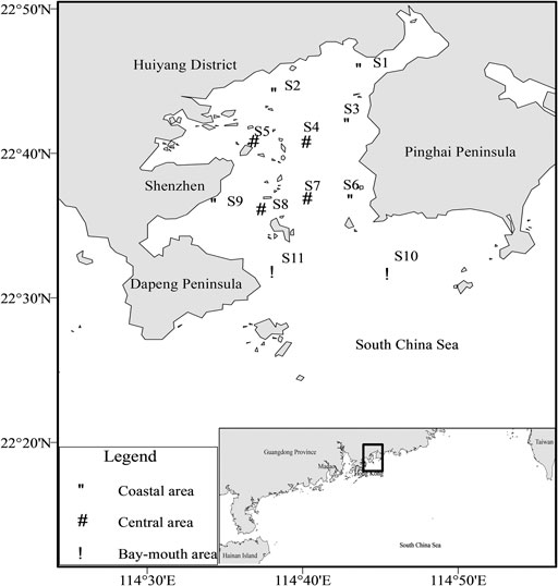
FIGURE 1. Map of sampling stations in Daya Bay.
Eleven stations were set in Daya Bay, among which the coast consists of five stations, namely, S1, S2, S3, S6, and S9; the middle of the bay consists of four stations, including S4, S5, S7, and S8; and the mouth of the bay comprises two stations, namely, S10 and S11 (Figure 1). Four voyage bottom trawl surveys were carried out in August 2016 (summer), December 2016 (winter), March 2017 (spring), and October 2017 (autumn). Along with fish collection, data on four environmental variables were obtained simultaneously from the stations. The water depth (m) of each station was obtained by a ship-borne sounder. The physical environment data such as sea surface salinity, sea surface temperature (°C), dissolved oxygen (DO, mg/L), and pH were measured by a YSI Pro Series multifunctional water quality meter. The environmental parameters and fishery resources investigations were based on “the specifications for the oceanographic survey” (GB/T12763-2007, China), “the specifications for marine monitoring” (GB17378-2007, China), “the specifications for coastal waters environmental monitoring norms” (HJ442-2008, China), and “the specifications for marine fishery resources survey” (SC/T9403-2012, China) and standardized the data. The survey vessel was a steel fishing boat with a power of 135 kW that was operated during the day. The sampling net was a single-vessel winged single-bag bottom trawl with a net mouth circumference of 102 m, net length of 50 m, on the framework of 51 m, under the outline of 51 m, and net mesh size of 2 cm. Each station was trawled one time and dragged 1 h, with an average hauling speed of 3.4 knots for all surveys. The catches were classified and identified on site, and the biological parameters such as the body length (BL, mm) and body weight (BW, 0.1 g) of each individual were immediately measured, and then the samples were frozen, stored on site, and transferred to the laboratory. Sampling and analysis were carried out according to the “Marine Biological Survey Code” (National Standardization Administration of the People’s Republic of China General Administration of Quality Supervision 2007).
Analytical Methods
Abundance–Biomass Comparison Curve
The ABC curve method analyzes the characteristics of the community under different disturbance conditions by calculating the distribution of species abundance and biomass using the W-statistic as a statistic of the ABC curve method (Yemane et al., 2005):
where Ai and Bi represent the cumulative numbers of the species number i and the cumulative percentage of biomass in the ABC curve, respectively, and S is the total number of species.
Sheldon-type BSS
In Sheldon-type BSS analysis, if the size of the smallest fish species is V, then the first particle size of fish ranges from V to 2V, the second size ranges from 2 to 4V, and so on. The fish size interval follows the base 2 logarithm and divides the fish size into different size levels (Sheldon et al., 1972). The Sheldon-type BSS is divided by the log2 conversion size interval as the abscissa, and the total biomass per unit area (m2) corresponding to each size group is converted by log2 as the ordinate (Jung and Houde 2005). This allows the biomass distribution to not rely on the fish size intervals, allowing comparisons of different fish communities, regardless of fish size (Macpherson et al., 2002). The fish community’s structural characteristics are reflected by the “peak shape” formed by the crests and troughs on the curve (Kerr and Dickie 2001).
Normalized Biomass Size Spectrum
In the NBSS, the horizontal axis is consistent with the Sheldon-type model, but the vertical axis is different. The vertical axis is the ratio of the total biomass (wet weight) of organisms in a specific weight category to the interval of weight changes in the category, all expressed on a logarithmic scale (Sprules and Munawar 1986). This logarithmic scale describes the characteristics of fish community structures mainly using the linear regression equation or parabolic equation parameters, which compare the differences among various fish communities and predict the future development of fish community conditions (Sprules and Munawar 1986; Kerr and Dickie 2001). When the community is in a stable state, the NBSS is a straight line (y = ax + b), where a represents the slope, indicating the relationship between biomass and the particle size of fish. Once a equals −1, it demonstrates that the fish biomass is consistent with the increase in the particle size. When a is less than −1, it indicates that the fish biomass decreases as the size increases. On the other hand, a greater than −1 reveals that the fish biomass increases with the increase in the grain size, while b represents the intercept, expressing the abundance and productivity of the fish community. The difference in b value represents the variance in the productivity level of different fish communities, for which the magnitude of the productivity level is positively correlated with the b value (Platt and Denman 1977; Guo et al., 2017). On the other hand, when the community is in an unstable state, the NBSS is a parabolic equation (y = ax2+bx + c), and a represents curvature which is affected by various factors such as the nutritional level, fishing, and breeding population (Macpherson and Gordoa 1996; Trebilco et al., 2013). R2 represents the determination coefficient of the fitting equation obtained by the linear or nonlinear model and describes the extent to which fish communities deviate from their steady state.
Data Analysis
The data of the survey were calibrated and analyzed by ArcGis10.3 software and SPSS19.0 statistical analysis software. According to the survey results of each station, the average body weight of fish of more than 9 g and less than 9 g at each station was calculated. Also, to map the fish body size distribution, an ArcGIS10.3 raster interpolation was used, which helps understand the characteristics of the distribution within the seascape.
Results
Fish Community Structure
A total of 131 fish species were collected, belonging to 13 orders, 53 families, and 84 genera, all of which belonged to the Osteichthyes class. Perciformes contained the largest number of species, with 71 species, accounting for 54.20% of the total species. The fish community of Daya Bay demonstrated significant seasonal changes, which are summarized in Table 1. The fish community mainly composed of Evynnis cardinalis and Callionymus richardsoni, which feed on benthic organisms; Trachurus japonicus and Apogon lineatus, which feed on plankton organisms; and Leiognathus brevirostris and Clupanodon punctatus larvae, which feed on plankton and benthic organisms. Overall, the fish structure presented miniaturization and a low-weight trend. The average individual mass of fish in the whole bay was 9 g. The distribution of the body size of small fish (<9 g) and large fish (>9 g) after grid interpolation showed that the abundance of large-sized fish reduced progressively from the east to the west coast of the gulf. On the other hand, the small-sized fish overall showed an increasing trend from the bay mouth area to the northern coastal waters. Moreover, the fish in the coral reef area and the bay mouth were the smallest in size, while the high-value area was in the eastern coastal waters. Overall, the fish in the littoral waters were comparatively large, while the fish in the middle and the mouth of the bay were relatively small (Figure 2).
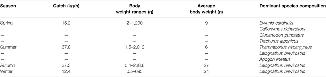
TABLE 1. Seasonal changes of the fish community structure in Daya Bay.
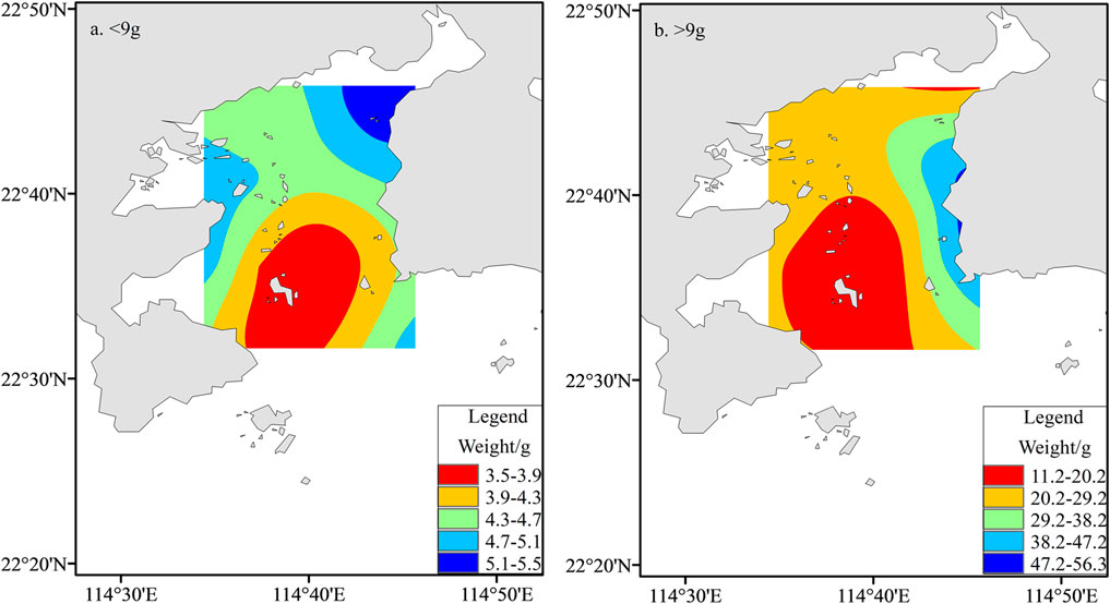
FIGURE 2. Spatial distribution of fish physically in two designated size classes in Daya Bay; (A) small fish <9 g wet weight; (B) large fish >9 g wet weight.
Abundance–Biomass Comparison Curve
There were significant seasonal variations and spatial differences in fish communities’ ABC curves of Daya Bay (Figure 3 and Figure 4). In the seasonal changes, the fish communities in spring, summer, and autumn were all in a critical disturbance state. The fish community consisted mainly of small-sized fish, while the winter fish community was in a moderate disturbance state. The fish community structure was better in winter than the other three seasons, and the W values of the four seasons were −0.07, −0.17, −0.08, and 0.17, respectively. In the spatial distribution, the coastal waters and the central waters were in a critical disturbance state, while the mouth of the bay was moderately disturbed. The W values of the coastal waters, central waters, and mouth waters were −0.10, −0.15, and −0.09, respectively. The coastal area was the most disturbed, followed by the central waters. Furthermore, the entire sea area was in a critical disturbance state throughout the year.
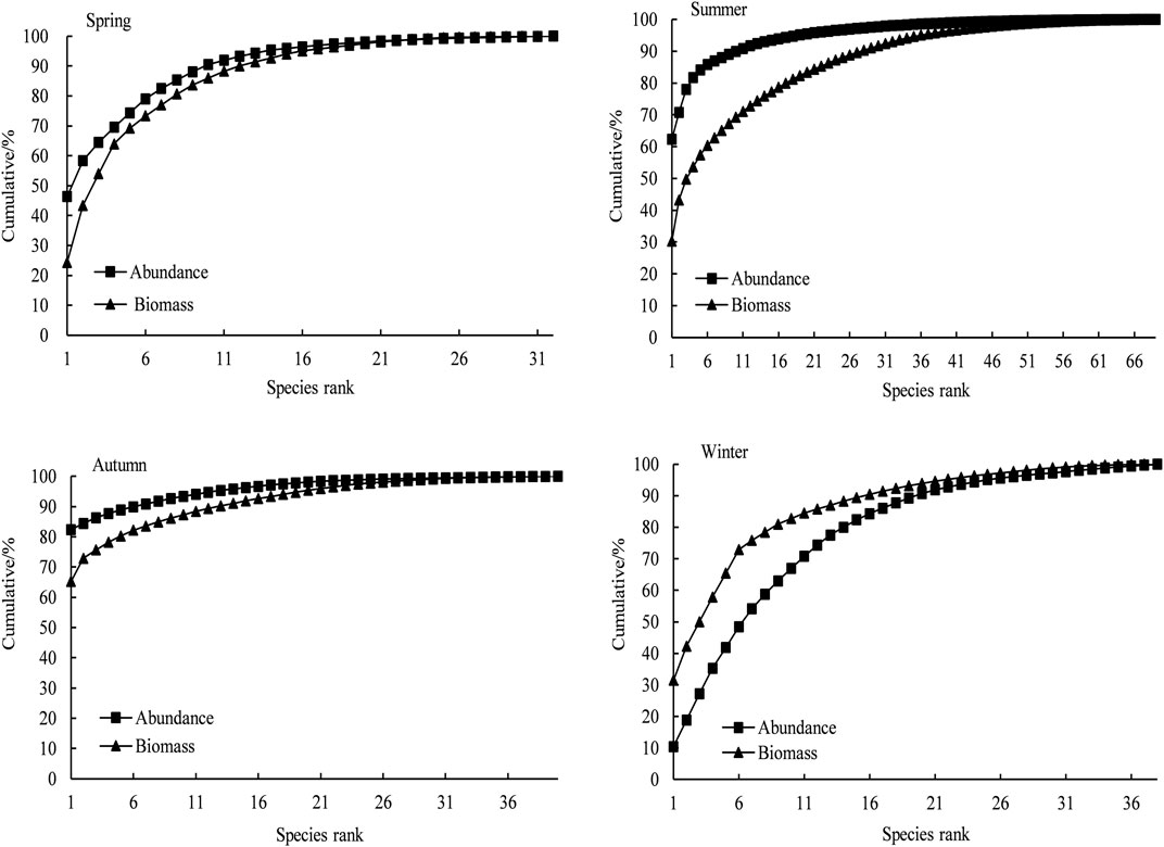
FIGURE 3. ABC curves of fish community in every season in Daya Bay.
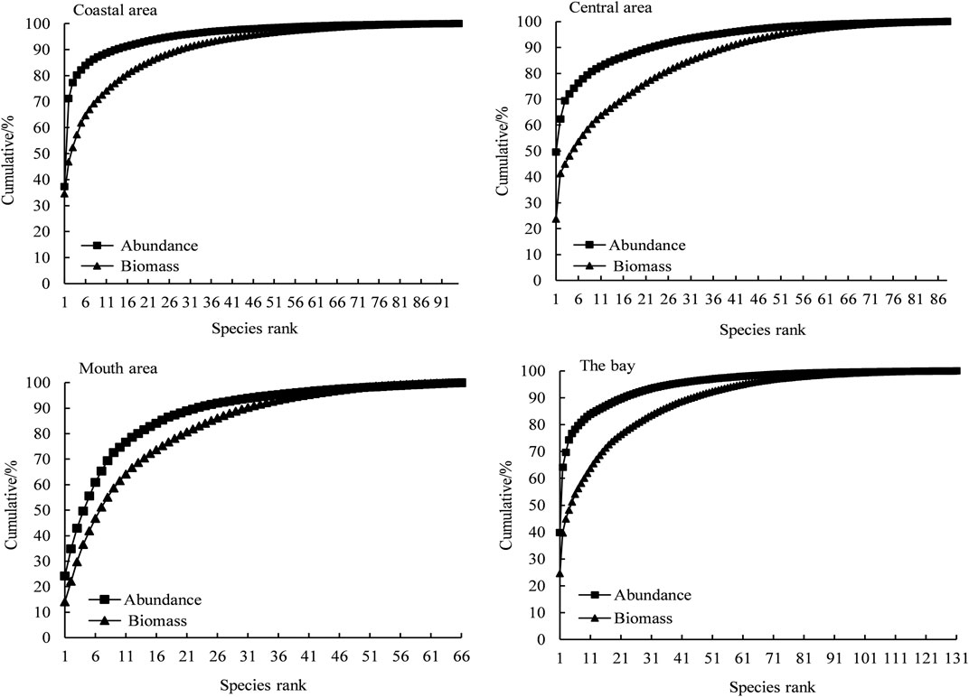
FIGURE 4. ABC curves of fish community in the region in Daya Bay.
Fish BSS
Fish BSS in Daya Bay
According to the survey results of four voyages, the BSS of fish in Daya Bay was constructed (Figure 5). The Sheldon-type BSS of fish was a single-peaked pattern with the grain size (log2 size bins) ranging between −2 and 10, where the fish were predominantly in the range of four to eight grain level. The size spectrum dome was located on the two to four grain level. Its corresponding body mass of fish ranged from 8 to 16 g, mainly composed of Leiognathus brevirostris, Callionymus meridionalis, Callionymus koreanus, Evynnis cardinalis, Trachurus japonicus, and other small fishes. Also, the curvature of the NBSS was −0.23 in Daya Bay.
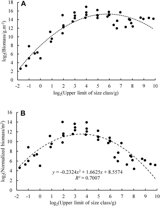
FIGURE 5. Biomass size spectrum of fish in Daya Bay; a. Sheldon; b. normalized.
Seasonal Changes of Fish BSS
The Sheldon-type BSS of the four seasons in Daya Bay showed an irregular sawtooth shape with evident seasonal variations (Figure 6, p < 0.05). In general, all four seasonal curves showed a unimodal pattern. Commonly in spring and winter, the peak and trough were interdependent, and the curve of BSS slightly fluctuated. Only one peak appeared in summer and autumn, without trough occurrence, and the curve fluctuated marginally. The fish size ranged from −2 to 10 in four seasons, ranging from −2 to 10 in spring, summer, and winter, while from −2 to 8 grain level in autumn.
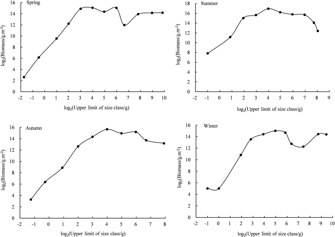
FIGURE 6. Biomass size spectra of fishes in every season in Daya Bay.
The NBSS of fish for all seasons was designed based on the analysis of fish biology data. All the regression results were significant (p < 0.05), and there were seasonal differences (Figure 7; Table 2). The curvature ranges of the NBSS of fish for the four seasons ranged from −0.33 to −0.19, of which spring curvature was the largest, followed by winter and autumn, and summer curvature was the smallest. The R2 ranged from 0.67 to 0.95, exhibiting the largest value in summer and the smallest in winter.

FIGURE 7. Normalized biomass spectra of fishes in every season in Daya Bay.
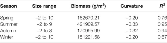
TABLE 2. Seasonal comparison of the normalized biomass particle size spectrum of fish in Daya Bay.
Spatial Changes of Fish BSS
The Sheldon-type BSS and NBSS of fish were constructed based on the survey data, the coastal area, the central region, and the bay mouth in Daya Bay with evident spatial changes (Figure 8 and Figure 9, p < 0.05). The Sheldon-type BSS in the three regions was a single peak, while the highest peaks in the coastal and central sea areas were in the two to four size range, and the highest peak in the bay waters was in the four to six size range. The fish size ranged from 2 to 10 grains, of which the coastal and bay mouth waters ranged from −2 to 10 grains, while the central waters ranged from 2 to 8 grains. The curvature of fish NBSS was in the range from −0.39 to −0.19, of which the coastal area was the largest, followed by the bay mouth (−0.27). The central area was the smallest; R2 ranged from 0.81 to 0.98, with the highest in the central region and the lowest in the coastal zone (Table 3).
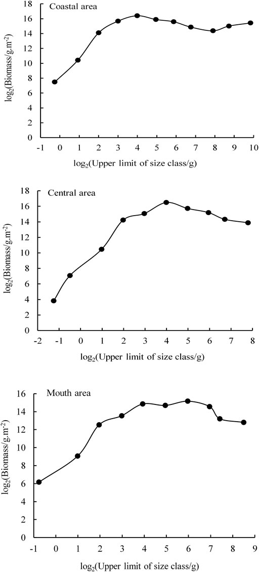
FIGURE 8. Sheldon type biomass size spectrum of fish in different areas of Daya Bay.

FIGURE 9. Normalized biomass size spectra of fish in different regions of Daya Bay.

TABLE 3. Spatial changes of the normalized biomass particle size spectrum of fish in Daya Bay.
Discussion
Ecological Indication of ABC Curve
The fish biomass dominance curve in Daya Bay was lower than the abundance dominance curve, indicating that the fish community structure was severely disturbed, and the fish community composed of small, fast-growing species that mature early. Throughout the year, spring, summer, and autumn seasons were in a severe disturbance state; however, winter was in a moderate state (Yemane et al., 2005). This was consistent with the findings of a previous study that the fish composition was mainly dominated by small-size fish such as Evynnis cardinalis, Callionymus koreanus, Clupanodon punctatus, Trachurus japonicus, Thamnaconus hypargyreus, and Leiognathus brevirostris, where the fish size structure showed a trend of miniaturization and low weight (Guo et al., 2018). Studies have also shown that the status of fish abundance is related to its reproductive rate, growth habits, seasonal differences in the living environment, and human activities (especially fishing) (Fenberg and Roy 2008; Li 2008; Rochet and Benoit 2012; Guo et al., 2018; Xu et al., 2020; Marrakchi et al., 2021). Considering the time of the investigation, the spring and summer seasons were before and after the South China Sea fishing moratorium, but summer was the most disturbed, while the fish community structure in spring was less disturbed than summer. The average fish weight (9 g) in spring was higher than that in summer (6 g). Besides, the spring and summer seasons were the main spawning periods for most fish in Daya Bay. Some fishes such as Clupanodon punctatus, Trachurus japonicus, Trichiurus lepturus, and Thryssadussumieri began reproduction considerably, which resulted in both fecundity and juveniles to reach the maximum during summer (Xu 1989; Lin et al., 2010; Cao et al., 2021; Lakshmikandan et al., 2021). In addition, the summer survey was conducted in the second week after the end of the fishing season. Overfishing by coastal fishers resulted in the caught being dominated by the high abundance of small-size fish in summer, in which their weight and quantity accounted for 47.5 and 72.8% of the total catches, respectively. Besides, the biomass dominance curve was lower than the abundance dominance curve, and the fish community was in a severe disturbance state. In winter, a small quantity of Acanthopagrus schlegelii, Gymnothorax hepaticus, Johnius distinctus, Pampus chinensis, Johniusbelangerii, and other large species were captured, with the average individual weighed more than 50 g, which was significantly higher than that in the other three seasons. Also, the community structure showed lower disturbances in winter than in the other three seasons, and the fish community was in a moderate state of disturbance due to the impact of low temperature, fish migration, and low fishing pressure. Remarkably, the coastal waters were affected by overfishing, resulting in a severe disturbance. In the middle of the bay, several island reefs provided a natural sanctuary for reef fish breeding (Wang and Zhao 2001), which was not conducive to bottom trawl fishing. Therefore, the degree of disturbance was relatively low, and moderate disturbance was observed.
Characteristics of Fish BSS in Daya Bay
Composition of Fish
The particle size of organisms is highly associated with the material and energy flow in marine ecosystems, the structure and function of biological communities, and physical and chemical processes (Belgrano and Brown 2002; Li 2002). Therefore, biologic particle size spectroscopy can be employed to reflect the structural composition of biologic communities (Marquet et al., 2005). The results of fish compositions of this study are shown in Table 4.
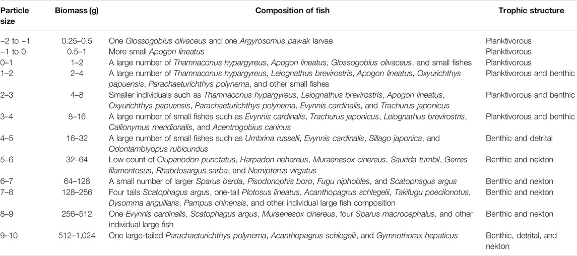
TABLE 4. Fish composition according to the particle size.
Ecological Characteristics of Fish Community Structure
The curve was larger in spring and winter and smaller in summer and autumn. The regression coefficient, R2, was small in spring and winter and was large in summer and autumn. The size ranges were wide in spring and winter and slightly smaller in summer and autumn, indicating that the fish community structure in spring and winter was composed of smaller size fishes than summer and autumn. In winter, the fish community structure was the least disturbed by human activities, while summer showed the highest human disturbances. Particularly, the coastal areas were the most affected areas by human activities, followed by the central bay area. The lowest degree of human disturbance was observed in the mouth of the bay, indicating that the fish community structure was unstable in the coastal zones, and the fish community structure was relatively stable in the central region and mouth of the bay.
The particle size is a prominent structural feature of fish communities and significantly reflects fish movement (Bainbridge 1958), predation (Lundvall et al., 1999; Scharf et al., 2000), reproduction (Woodward et al., 2005), the mortality rate (Peterson and Wroblewski 1984), and fishing (Fenberg and Roy 2008). The trophic level of organisms is closely related to the fish size (Jennings et al., 2001; Trebilco et al., 2013). Mainly, the fish grain size structure is influenced by the productivity level of the area, fishing intensity (especially overfishing), species compensation ratio (number of breeding population), and environment, all of which influence the BSS of fish (Jennings and Reynolds 2007; Fenberg and Roy 2008; Wang et al., 2013). In this study, the main fish species in the smallest grain size (2–0 grain size) during spring, summer, autumn, and winter seasons were Glossogobius olivaceus, Apogon lineatus, Argyrosomus pawak, and Parachaeturichthys polynema, respectively. Since the biomass size was small at this grain level, it significantly influenced the curvature of its NBSS. Predominantly, the biomass grain level in the coastal waters, the middle bay area, and the mouth area was the smallest, and the fish species with the highest biomass contribution rates were Apogon lineatus, Argyrosomus pawak, and Pterois volitans. Consequently, this affected the curvature of the NBSS. In summer and autumn, Daya Bay shows high productivity, and spawning fishes begin to spawn abundantly in summer, resulting in both fecundity and juveniles to reach their peaks (Xu 1989; Lin et al., 2010). Besides, from June to August, due to the fishing moratorium period in the South China Sea, the protection of fish resources resulted in highest fish abundance, and biomass size and upwelling were observed on the east coast of Guangdong (Xu 1989). Also, the South China Sea invasion trend showed increased nutrition supplementation in the bay, which provides a well-nourished environment for fish and plankton growth (Wu et al., 2007; Lakshmikandan et al., 2020; Barati et al., 2021; Lakshmikandan et al., 2021), resulting in the larger mean biomass size of fish in summer and autumn than in spring and winter. However, after summer fishing moratorium, the increase in fishing intensity reduced the amount of large-size fishes (Guo et al., 2018), coupled with the replenishment of spawning fishes (Xu 1989), and resulted in a fish community comprising small-sized fishes. And overfishing was the main reason for the relatively steep curvature of the NBSS. In spring and winter, the productivity of Daya Bay was comparatively low, and fishing was moderately less, wherein fishes such as Clupanodon punctatus began spawning predominantly. In winter, most commercial fishes such as Trachurus japonicus, Pagrosomus major, Formio niger, and Decapterus maruadsi migrated from the bay to the deep waters outside the bay for overwintering (Xu 1989), while more large fishes such as Sparus macrocephalus were captured, which resulted in a comparatively uniform distribution of fish size and a relatively flat NBSS curvature. Also, the particle size structure was superior to other seasons as the grain size range was larger. Coastal waters were disturbed by fishing, and the coastline and fish habitats were damaged (Wang et al., 2010). The degree of disturbance was highest, and there was a lack of small-size species ranging from −2 to −1, which led to a steeper curve of the BSS. In the middle of the bay, several island reefs were not easy to catch on the bottom trawling. The degree of disturbance was rather small, and the community was reasonably stable, resulting in relatively flat curvature. The water depth was higher in bay mouth than the nearshore and the middle, and human activities were relatively low, resulting in a more stable fish community structure. Ma et al. (2014) studied the number size spectra (NSS) of planktons in Daya Bay during summer and winter. The result indicated that the hot water discharges from nuclear power plants and agricultural wastewater releases significantly affected the plankton biomass size distribution and NSS patterns. The study demonstrated the application of BSS in studying the impacts of human disturbances on the marine ecosystem and also indicated that the particle size can be used as an ecological indicator to reflect the stability of the community structure.
Peaks are usually formed in small- and large-size species, and troughs are formed at their junctions (Schwinghamer 1981). It was suggested that the distribution of peaks and troughs is not a fixed pattern (Dolbeth et al., 2014). Their formation mainly depends on the appearance of key species in different seasons, rather than the living environments of the communities. In this study, the wave peak corresponds to a large number of small species or a low number of large species, and the troughs were at the intersection of small and large species. Also the capture of specific species in the community affected the peak shape of the NBSS, which was consistent with a previous study (Shen 2010). The corresponding fish species in the two to four size class exhibited the highest biomass abundance, which accounted for 24.76% of the total biomass, mainly consisting of highly abundant small fishes. For instance, the catch quantity and weight of Leiognathus brevirostris were the highest, accounting for 37.96 and 37.85% of the total catch, respectively. Also, the fish biomass on the two to four grain level exhibited an increasing trend, while the fish biomass on the 4–10 scales showed a decreasing trend, resulting in a single-peak pattern of the Sheldon-type BSS in Daya Bay. In summer, largely small-sized fishes, such as Evynnis cardinalis and Leiognathus brevirostris, were captured, and the catch weight reached the maximum, making it the highest peak in the two to four grains. In winter, one Acanthopagrus schlegelii and one Pampus chinensis were captured on the six to eight scale, and the biomass size was the smallest, resulting in a trough occurrence.
The continuous fish size spectrum analysis provides a straightforward mechanism to understand the condition of the aquatic ecosystem (Benoı̂t and Rochet 2004; Maury et al., 2007). It lowers the intricacy of food webs, indicates the slope of NBSS, and demonstrates that the intercepts are useful to describe the characteristics of ecosystem status (Guiet et al., 2016). It is different from traditional research methods and does not rely on taxonomy knowledge. Moreover, it minimizes the calculation errors caused by the uncertainty of classification and identification, while enhances our understanding of marine ecosystem characteristics and fish species in ecological and physiological processes. Additionally, it forecasts and evaluates productivity, production, and distribution of fish community and assists in monitoring environmental changes (Borgmann 1982; Boudreau and Dickie 1992; Cyr and Peters 1996; Trebilco et al., 2013; Guo et al., 2017). It is an innovative method to study fish communities. It can be applied to study the influences of fishing, reproduction tactics, or environmental alternation at various times on the fish community. Also, evaluating the influences of climatic variations on the marine ecosystem can be considered another application (Woodworthjefcoats et al., 2013; Guénette et al., 2014). On the other hand, the structure of species diversity in fish communities considerably influences the marine ecosystem’s performance, sensitivity to disturbances, and resilience (Blanchard et al., 2011), which urges the development of size-based uniqueness of the fish size spectrum (Guiet et al., 2016). In future research, it is essential to improve and advance the fish size spectrum method for further development and protect marine fishery resources.
Conclusion
The Sheldon-type BSS of fish in Daya Bay was a unimodal pattern, consisting of the fish size ranging from −2 to 10 grain level. Fishes in the range of four to eight size class were relatively abundant. The highest peak belonged to the two to four grain level and predominantly composed of Leiognathus brevirostris, Callionymus meridionalis, Callionymus koreanus, Evynnis cardinalis, Trachurus japonicus, and other small fishes. The curve of the BSS was relatively flat with large curvature in spring and winter. The curves in summer and autumn were comparatively steep, and the curvature was small. The characteristics of fish BSS were significantly affected by the number and size of the breeding population, the trophic level and migratory habits of fish, and other life history characteristics as well as human disturbance (fishing), among which overfishing was the dominant factor. The ABC curve showed that the fish community in Daya Bay was in a state of serious disturbance throughout the year.
Data Availability Statement
The raw data supporting the conclusions of this article will be made available by the authors, without undue reservation.
Ethics Statement
Ethical review and approval was not required for the animal study because the study was conducted by only measuring the size and identifying fish type by their appearance in the ecosystem. No experiment was conducted on the studied fishes.
Author Contributions
SX, JF, TX, and CL contributed to the conception and design of this study. JG, KW, TX, BB, and YL developed the method, acquired the data, and wrote the first draft of the manuscript. JF and YXu ran the analyses. SX and BB provided feedback on analysis. SX, BB, and CL provided revisions and editing. All authors read and approved the submitted version.
Funding
This researched was supported by the National Key R&D Program of China (2018YFD0900902), Fundamental and Applied Fundamental Research Major Program of Guangdong Province (2019B030302004-05), Key Special Project for Introduced Talents Team of Southern Marine Science and Engineering Guangdong Laboratory (Guangzhou) (GML2019ZD0605), Science and Technology Planning Project of Guangdong Province (2019B121201001), Central Public-interest Scientific Institution Basal Research Fund, CAFS (2020TD16), Central Public-interest Scientific Institution Basal Research Fund, SCSFRI, CAFS (2021SD04), and Financial Fund of the Ministry of Agriculture and Rural Affairs, P. R. of China (NFZX 2018).
Conflict of Interest
The authors declare that the research was conducted in the absence of any commercial or financial relationships that could be construed as a potential conflict of interest.
References
Bainbridge, R. (1958). The Speed of Swimming of Fish as Related to Size and to the Frequency and Amplitude of the Tail Beat. J. Exp. Biol. 35 (1), 109–133. doi:10.1242/jeb.35.1.109
Barati, B., Zeng, K., Baeyens, J., Wang, S., Addy, M., Gan, S.-Y., et al. (2021). Recent Progress in Genetically Modified Microalgae for Enhanced Carbon Dioxide Sequestration. Biomass and Bioenergy 145, 105927. doi:10.1016/j.biombioe.2020.105927
Belgrano, A., and Brown, J. H. (2002). Oceans Under the Macroscope. Nature. 419 (6903), 128–129. doi:10.1038/419128a
Benoı̂t, E., and Rochet, M.-J. (2004). A Continuous Model of Biomass Size Spectra Governed by Predation and the Effects of Fishing on them. J. Theor. Biol. 226 (1), 9–21. doi:10.1016/S0022-5193(03)00290-X
Blanchard, F., LeLoc'h, F., Hily, C., and Boucher, J. (2004). Fishing Effects on Diversity, Size and Community Structure of the Benthic Invertebrate and Fish Megafauna on the Bay of Biscay Coast of France. Mar. Ecol. Prog. Ser. 280 (10), 249–260. doi:10.3354/meps280249
Blanchard, J. L., Law, R., Castle, M. D., and Jennings, S. (2011). Coupled Energy Pathways and the Resilience of Size-Structured Food Webs. Theor. Ecol. 4 (3), 289–300. doi:10.1007/s12080-010-0078-9
Borgmann, U. (1982). Particle-Size-Conversion Efficiency and Total Animal Production in Pelagic Ecosystems. Can. J. Fish. Aquat. Sci. 39 (5), 668–674. doi:10.1139/f82-096
Boudreau, P. R., and Dickie, L. M. (1992). Biomass Spectra of Aquatic Ecosystems in Relation to Fisheries Yield. Can. J. Fish. Aquat. Sci. 49 (8), 1528–1538. doi:10.1139/f92-169
Cao, B., Yuan, J., Jiang, D., Wang, S., Barati, B., Hu, Y., et al. (2021). Seaweed-derived Biochar with Multiple Active Sites as a Heterogeneous Catalyst for Converting Macroalgae into Acid-free Biooil Containing Abundant Ester and Sugar Substances. Fuel. 285, 119164. doi:10.1016/j.fuel.2020.119164
Cyr, H., and Peters, R. H. (1996). Biomass-size Spectra and the Prediction of Fish Biomass in Lakes. Can. J. Fish. Aquat. Sci. 53 (5), 994–1006. doi:10.1139/f96-033
Dolbeth, M., Raffaelli, D., and PardalÂ, M. Â. (2014). Patterns in Estuarine Macrofauna Body Size Distributions: The Role of Habitat and Disturbance Impact. J. Sea Res. 85, 404–412. doi:10.1016/j.seares.2013.07.012
Emmrich, M., Brucet, S., Ritterbusch, D., and Mehner, T. (2011). Size Spectra of lake Fish Assemblages: Responses along Gradients of General Environmental Factors and Intensity of Lake-use. Freshw. Biol. 56 (11), 2316–2333. doi:10.1111/j.1365-2427.2011.02658.x
Fenberg, P. B., and Roy, K. (2008). Ecological and Evolutionary Consequences of Size-Selective Harvesting: How Much Do We Know? Mol. Ecol. 17 (1), 209–220. doi:10.1111/j.1365-294x.2007.03522.x
Graham, N., Dulvy, N., Jennings, S., and Polunin, N. (2005). Size-spectra as Indicators of the Effects of Fishing on Coral Reef Fish Assemblages. Coral Reefs. 24 (1), 118–124. doi:10.1007/s00338-004-0466-y
Guénette, S., Araújo, J. N., and Bundy, A. (2014). Exploring the Potential Effects of Climate Change on the Western Scotian Shelf Ecosystem, Canada. J. Mar. Syst. 134 (3), 89–100. doi:10.1016/j.jmarsys.2014.03.001
Guiet, J., Poggiale, J.-C., and Maury, O. (2016). Modelling the Community Size-Spectrum: Recent Developments and New Directions. Ecol. Model. 337, 4–14. doi:10.1016/j.ecolmodel.2016.05.015
Guo, J., Chen, Z., Xu, Y., Xu, S., Huang, Z., and Li, C. (2018). The Effects of Anthropogenic Activities on the Diversity and Succession of Fish Community in Daya Bay. J. Fish. Sci. China. 25 (3), 595–607. doi:10.3724/sp.j.1118.2018.17277
Guo, J. Z., Chen, Z. Z., and Xu, S. N. (2017). Advances in Fish Particle Size Spectra Study. Mar. Fish. 39 (5), 582–591. doi:10.13233/j.cnki.mar.fish.2017.05.012
Jennings, S., Pinnegar, J. K., Polunin, N. V. C., and Boon, T. W. (2001). Weak Cross-Species Relationships Between Body Size and Trophic Level Belie Powerful Size-Based Trophic Structuring in Fish Communities. J. Anim. Ecol. 70 (6), 934–944. doi:10.1046/j.0021-8790.2001.00552.x
Jennings, S., Pinnegar, J., Polunin, N., and Warr, K. (2002). Linking Size-Based and Trophic Analyses of Benthic Community Structure. Mar. Ecol. Prog. Ser. 226, 77–85. doi:10.3354/meps226077
Jennings, S., and Reynolds, J. D. (2007). Body Size, Exploitation and Conservation of marine organisms//Body size:The Structure and Function of Aquatic Ecosystems. Cambridge, UK: Cambridge University Press
Jung, S., and Houde, E. D. (2005). Fish Biomass Size Spectra in Chesapeake Bay. Estuaries. 28 (2), 226–240. doi:10.1007/bf02732857
Kerr, S. R., and Dickie, L. M. (2001). The Biomass Spectrum : A Predator-Prey Theory of Aqautic Production. New York, NY: Columbia University Press.
Lakshmikandan, M., Murugesan, A. G., Wang, S., Abomohra, A. E.-F., Jovita, P. A., and Kiruthiga, S. (2020). Sustainable Biomass Production under CO2 Conditions and Effective Wet Microalgae Lipid Extraction for Biodiesel Production. J. Clean. Prod. 247, 119398. doi:10.1016/j.jclepro.2019.119398
Lakshmikandan, M., Wang, S., Murugesan, A. G., Saravanakumar, M., and Selvakumar, G. (2021). Co-cultivation of Streptomyces and Microalgal Cells as an Efficient System for Biodiesel Production and Bioflocculation Formation. Bioresour. Techn. 332, 125118. doi:10.1016/j.biortech.2021.125118
Li, C. H., Xu, S. N., Du, F. Y., and Li, L. (2015). Responses of the Daya Bay Ecosystem to Human Activities and Health Assessment. Chin. Fish. Qual. Stand. 5 (1), 1–10.
Li, S. F. (2008). Status of Fish Community in East China Sea Using the Method of Abundance- Biomass Comparison (ABC) curve. J. Fish. Sci. China 15 (1), 136–144. doi:10.3321/j.issn:1005-8737.2008.01.018
Li, W. K. W. (2002). Macroecological Patterns of Phytoplankton in the Northwestern North Atlantic Ocean. Nature. 419 (6903), 154–157. doi:10.1038/nature00994
Lin, Z. J., Wang, X. H., and Jiang, Y. E. (2010). Distribution and Species Composition of Fish Eggs in Daya Bay. J. Fish. Sci. China 17 (3), 543–550.
Lundvall, D., Svanbäck, R., Persson, L., and Byström, P. (1999). Size-dependent Predation in Piscivores: Interactions Between Predator Foraging and Prey Avoidance Abilities. Can. J. Fish. Aquat. Sci. 56 (7), 1285–1292. doi:10.1139/f99-058
Ma, Y. E., Ke, Z. X., Huang, L. M., and Tan, Y. H. (2014). Identification of Human-Induced Perturbations in Daya Bay, China: Evidence from Plankton Size Structure. Cont. Shelf. Res. 72, 10–20. doi:10.1016/j.csr.2013.10.012
Macpherson, E., and Gordoa, A. (1996). Biomass Spectra in Benthic Fish Assemblages in the Benguela System. Mar. Ecol. Prog. Ser. 138 (1-3), 27–32. doi:10.3354/meps138027
Macpherson, E., Gordoa, A., and Garcı́a-Rubies, A. (2002). Biomass Size Spectra in Littoral Fishes in Protected and Unprotected Areas in the NW Mediterranean. Estuarine, Coastal Shelf Sci. 55 (5), 777–788. doi:10.1006/ecss.2001.0939
Marquet, P. A., Quiñones, R. A., Abades, S., Labra, F., Tognelli, M., Arim, M., et al. (2005). Scaling and Power-Laws in Ecological Systems. J. Exp. Biol. 208 (9), 1749–1769. doi:10.1242/jeb.01588
Marrakchi, F., Fazeli Zafar, F., Wei, M., and Wang, S. (2021). Cross-linked FeCl3-Activated Seaweed carbon/MCM-41/alginate Hydrogel Composite for Effective Biosorption of Bisphenol A Plasticizer and Basic Dye from Aqueous Solution. Bioresour. Techn. 331, 125046. doi:10.1016/j.biortech.2021.125046
Maury, O., Faugeras, B., Shin, Y.-J., Poggiale, J.-C., Ari, T. B., and Marsac, F. (2007). Modeling Environmental Effects on the Size-Structured Energy Flow through marine Ecosystems. Part 1: The Model. Prog. Oceanography 74 (4), 479–499. doi:10.1016/j.pocean.2007.05.002
National Standardization Administration of the People's Republic of China General Administration of Quality Supervision, I. a. Q (2007). Specifications for Oceanographic Survey—Part 6: Marine Biological Survey. Beijing.
Pagola-Carte, S. (2004). ABC Method and Biomass Size Spectra: What about Macrozoobenthic Biomass on Hard Substrata? Hydrobiologia. 527 (1), 163–176. doi:10.1023/b:hydr.0000043199.12496.2d
Peterson, I., and Wroblewski, J. S. (1984). Mortality Rate of Fishes in the Pelagic Ecosystem. Can. J. Fish. Aquat. Sci. 41 (7), 1117–1120. doi:10.1139/f84-131
Platt, T., and Denman, K. (1977). Organisation in the Pelagic ecosystem. Helgolnder Wissenschaftliche Meeresunter suchungen. 30 (1-4), 575–581. doi:10.1007/bf02207862
Rochet, M.-J., and Benoît, E. (2012). Fishing Destabilizes the Biomass Flow in the marine Size Spectrum. Proc. R. Soc. B. 279 (1727), 284–292. doi:10.1098/rspb.2011.0893
Romero, G. Q., Marino, N. A. C., A. Andrew M. MacDonald, A. A. M., Céréghino, R., Trzcinski, M. K., and Mercado, D. A. (2020). Extreme Rainfall Events Alter the Trophic Structure in Bromeliad Tanks Across the Neotropics. Nat. Commun. 11, 3215. doi:10.1038/s41467-020-17036-4
Scharf, F., Juanes, F., and Rountree, R. (2000). Predator Size-Prey Size Relationships of marine Fish Predators: Interspecific Variation and Effects of Ontogeny and Body Size on Trophic-Niche Breadth. Mar. Ecol. Prog. Ser. 208 (1), 229–248. doi:10.3354/meps208229
Schwinghamer, P. (1981). Characteristic Size Distributions of Integral Benthic Communities. Can. J. Fish. Aquat. Sci. 38 (10), 1255–1263. doi:10.1139/f81-167
Sheldon, R. W., Prakash, A., and Sutcliffe, W. H. (1972). The Size Distribution of Particles in the Ocean1. Limnol. Oceanogr. 17 (3), 327–340. doi:10.4319/lo.1972.17.3.0327
Sheldon, R. W., Sutcliffe Jr., W. H., and Paranjape, M. A. (1977). Structure of Pelagic Food Chain and Relationship Between Plankton and Fish Production. J. Fish. Res. Bd. Can. 34 (12), 2344–2353. doi:10.1139/f77-314
Shen, G. Y. (2010). Marine Ecology. 3rd Edition. Beijing: Science Press. doi:10.1109/iccsit.2010.5563701
Sprules, W. G., Brandt, S. B., Stewart, D. J., Munawar, M., Jin, E. H., and Love, J. (1991). Biomass Size Spectrum of the Lake Michigan Pelagic Food Web. Can. J. Fish. Aquat. Sci. 48 (1), 105–115. doi:10.1139/f91-015
Sprules, W. G., and Munawar, M. (1986). Plankton Size Spectra in Relation to Ecosystem Productivity, Size, and Perturbation. Can. J. Fish. Aquat. Sci. 43 (9), 1789–1794. doi:10.1139/f86-222
Trebilco, R., Baum, J. K., Salomon, A. K., and Dulvy, N. K. (2013). Ecosystem Ecology: Size-Based Constraints on the Pyramids of Life. Trends Ecol. Evol. 28 (7), 423–431. doi:10.1016/j.tree.2013.03.008
Wang, L. R., and Zhao, H. T. (2001). The General Characteristics of the Coral Reef ecosystem. Chin. J. Ecol. 20 (6), 41–45.
Wang, X. H., Du, F. Y., Qiu, Y. S., Li, C. H., Sun, D. R., and Jia, X. P. (2010). Variations of Fish Species Diversity, Faunal Assemblage, and Abundances in Daya Bay in 1980-2007. Chin. J. Appl. Ecol. 21 (9), 2403–2410.
Wang, X. H., Du, F. Y., Qiu, Y. S., and Li, C. H. (2005). Study on the Ecosystem Model of Daya Bay I. A Preliminary Approach on Energy Flow model. South China Fish. Sci. 1 (3), 1–8.
Wang, Y. Z., Sun, D. R., Jia, X. P., and Huang, Z. R. (2013). Influence of Fishing Pressure and Climate Change on Filefish Catches in East China Sea. South China Fish. Sci. 9 (1), 8–15. doi:10.3969/j.issn.2095-0780.2013.01.002
Wang, Z. H., Qi, Y. Z., Chen, J. F., Xu, N., and Yang, Y. F. (2006). Phytoplankton Abundance, Community Structure and Nutrients in Cultural Areas of Daya Bay, South China Sea. J. Mar. Syst. 62 (1-2), 85–94. doi:10.1016/j.jmarsys.2006.04.008
Warwick, R. M. (1986). A New Method for Detecting Pollution Effects on Marine Macrobenthic Communities. Mar. Biol. 92 (4), 557–562. doi:10.1007/bf00392515
Warwick, R. M., and Clarke, K. R. (1994). Relearning the ABC: Taxonomic Changes and Abundance/biomass Relationships in Disturbed Benthic Communities. Mar. Biol. 118 (4), 739–744. doi:10.1007/bf00347523
Warwick, R. M., Pearson, T. H., and Ruswahyuni, fnm. (1987). Detection of Pollution Effects on Marine Macrobenthos: Further Evaluation of the Species Abundance/biomass Method. Mar. Biol. 95 (2), 193–200. doi:10.1007/bf00409005
Wijeyaratne, W. M. D. N., and Bellanthudawa, B. K. A. (2018). Abundance-Biomass Comparison Approach to Assess the Environmental Stressors in Diyawannawa Wetland in Monsoonal and Non-monsoonal Seasons. Sri Lanka J. Aquat. 23 (2), 135. doi:10.4038/sljas.v23i2.7555
Woodward, G., Ebenman, B., Emmerson, M., Montoya, J., Olesen, J., Valido, A., et al. (2005). Body Size in Ecological Networks. Trends Ecol. Evol. 20 (7), 402–409. doi:10.1016/j.tree.2005.04.005
Woodworth-Jefcoats, P. A., Polovina, J. J., Dunne, J. P., and Blanchard, J. L. (2013). Ecosystem Size Structure Response to 21st Century Climate Projection: Large Fish Abundance Decreases in the Central North Pacific and Increases in the California Current. Glob. Change Biol. 19 (3), 724–733. doi:10.1111/gcb.12076
Wu, R. H., Cai, S. Q., Wang, S. A., and Zhang, W. J. (2007). Three-dimensional Numerical Simulation of Tidal Current and Residual Current at Daya Bay. J. Trop. Oceanography 26 (3), 18–23. doi:10.3969/j.issn.1009-5470.2007.03.003
Xu, G. Z. (1989). Environments and Resources of Daya Bay. Heifei, China: Anhui Science and Technology Press. doi:10.1051/esomat/198906004
Xu, S. N., Guo, J. Z., Fan, J. T., Xu, Y. W., Su, L., and Li, C. H. (2020). Annual Variation in Fish Biomass Size Spectrum in Daya Bay, South China Sea in summer. South China Fish. Sci. 16 (4), 28–37. doi:10.12131/20200016
Keywords: fish communities, biomass size spectrum, ABC curve, Daya Bay, trawl surveys
Citation: Xu S, Guo J, Liu Y, Fan J, Xiao Y, Xu Y, Li C and Barati B (2021) Evaluation of Fish Communities in Daya Bay Using Biomass Size Spectrum and ABC Curve. Front. Environ. Sci. 9:663169. doi: 10.3389/fenvs.2021.663169
Received: 02 February 2021; Accepted: 25 May 2021;
Published: 15 June 2021.
Edited by:
Chao Song, Chinese Academy of Fishery Sciences, ChinaReviewed by:
Wentao Li, Ocean University of China, ChinaZhixin Ke, South China Sea Institute of Oceanology, Chinese Academy of Sciences, China
Copyright © 2021 Xu, Guo, Liu, Fan, Xiao, Xu, Li and Barati. This is an open-access article distributed under the terms of the Creative Commons Attribution License (CC BY). The use, distribution or reproduction in other forums is permitted, provided the original author(s) and the copyright owner(s) are credited and that the original publication in this journal is cited, in accordance with accepted academic practice. No use, distribution or reproduction is permitted which does not comply with these terms.
*Correspondence: Shannan Xu, eHVzaGFubmFuQHNjc2ZyaS5hYy5jbg==; Bahram Barati, QmFocmFtYmFyYXRpLmVkdUBnbWFpbC5jb20=