
94% of researchers rate our articles as excellent or good
Learn more about the work of our research integrity team to safeguard the quality of each article we publish.
Find out more
ORIGINAL RESEARCH article
Front. Environ. Sci. , 01 April 2021
Sec. Environmental Informatics and Remote Sensing
Volume 9 - 2021 | https://doi.org/10.3389/fenvs.2021.642906
This article is part of the Research Topic Emerging Technologies and Techniques for Remote Sensing of Coastal and Inland Waters View all 14 articles
 John Haskins1
 Charlie Endris2
 Alexandra S. Thomsen1,3*
 Fuller Gerbl1,2
 Monique C. Fountain1
 Kerstin Wasson1,4
Monitoring of environmental restoration is essential to communicate progress and improve outcomes of current and future projects, but is typically done in a very limited capacity due to budget and personnel constraints. Unoccupied aerial vehicles (UAVs) have been used in a variety of natural and human-influenced environments and have been found to be time- and cost-efficient, but have not yet been widely applied to restoration contexts. In this study, we evaluated the utility of UAVs as an innovative tool for monitoring tidal marsh restoration. We first optimized methods for creating high-resolution orthomosaics and Structure from Motion digital elevation models from UAV imagery by conducting experiments to determine an optimal density of ground control points (GCPs) and flight altitude for UAV monitoring of topography and new vegetation. We used elevation models and raw and classified orthomosaics before, during, and after construction of the restoration site to communicate with various audiences and inform adaptive management. We found that we could achieve 1.1 cm vertical accuracy in our elevation models using 2.1 GCPs per hectare at a flight altitude of 50 m. A lower flight altitude of 30 m was more ideal for capturing patchy early plant cover while still being efficient enough to cover the entire 25-hectare site. UAV products were valuable for several monitoring applications, including calculating the volume of soil moved during construction, tracking whether elevation targets were achieved, quantifying and examining the patterns of vegetation development, and monitoring topographic change including subsidence, erosion, and creek development. We found UAV monitoring advantageous for the ability to survey areas difficult to access on foot, capture spatial variation, tailor timing of data collection to research needs, and collect a large amount of accurate data rapidly at relatively low cost, though with some compromise in detail compared with field monitoring. In summary, we found that UAV data informed the planning, implementation and monitoring phases of a major landscape restoration project and could be valuable for restoration in many habitats.
Human activities including land conversion, resource exploitation, pollution, species introductions, and hydrologic alteration have changed ecosystems globally (Halpern et al., 2008; Gedan et al., 2009). Loss of foundation species is particularly concerning because these species provide habitat and modulate ecosystem processes (Dayton, 1972; Ellison, 2019). In response to negative anthropogenic effects on landscapes, land managers are increasingly undertaking restoration projects to support recovery of ecosystems and the valuable services they provide (Gedan et al., 2009; Palmer et al., 2016). A key element of environmental restoration is recovery of foundation species due to their influential ecological roles (Pastorok et al., 1997). When foundation species distributions are limited by environmental gradients such as moisture or salinity, restoration managers must design sites with appropriate landscape characteristics so that the desired species can successfully establish (Pastorok et al., 1997; Yando et al., 2019).
Monitoring is a critical component of any type of restoration (Pastorok et al., 1997). Restoration projects are often required by funders or permitters to set quantitative targets and monitor progress toward those goals (McDonald et al., 2016). Using monitoring data, restoration managers and scientists can conduct adaptive management and better understand the ecological processes driving restoration success (McDonald et al., 2016). Managers can also leverage monitoring data to engage community audiences by sharing information about local projects. In the past, monitoring tools consisted primarily of traditional field survey techniques, which are often time-consuming (Chabot and Bird, 2013), or remote sensing products available from airplanes or satellites, which are often only available at low spatial and temporal resolution (Roegner et al., 2008; Anderson and Gaston, 2013; Johnston, 2019). Despite its importance, monitoring of many restoration projects is fairly limited. Managers may only be able to conduct the minimum amount of monitoring that satisfies permit requirements (Zedler, 2000b) due to staffing limitations or funding restrictions that limit the amount or percentage of funds available. Unoccupied aerial vehicles (UAVs) offer a less expensive alternative to traditional methods, and UAV methods are beginning to be explored in restoration projects (Knoth et al., 2013; Marteau et al., 2017; Buters et al., 2019a; Padró et al., 2019a; Reis et al., 2019; Pérez et al., 2020).
Restoration monitoring across a variety of habitat types often includes both physical and biological elements (Pastorok et al., 1997; Roegner et al., 2008). Elevation is a major physical monitoring component in restoration (Roegner et al., 2008) given its key role in structuring ecological communities (Watson, 1835). Microtopography (variability on the scale of ∼1 cm to 1 m) and drainage patterns are also critical in restoration planning and monitoring. These factors influence hydrologic conditions (Jarzemsky et al., 2013), soil moisture and temperature (Diefenderfer et al., 2018), with implications for survival of plantings and natural colonization in restoration (Barry et al., 1996). Foundation species are a key biological monitoring target because in providing habitat for other species, they have a strong impact on the outcome of restoration (Pastorok et al., 1997).
Tidal marshes are a major habitat type targeted for restoration due to extensive losses globally (Gedan et al., 2009). Halophytic plants are important foundation species in marshes, with most only flourishing in a very narrow range of elevation, between mean high water and mean higher high water (Larson, 2001). Human activities that cause the landscape elevation to decrease, including diking and draining and groundwater overdraft, are common drivers of tidal marsh loss (Kennish, 2001; Kirwan and Megonigal, 2013). Accelerated sea level rise and restrictions to sediment supply also lead to loss of elevation relative to water levels (Kirwan and Megonigal, 2013; Weston, 2014; Watson et al., 2017). Therefore, a major component of marsh restoration is establishing appropriate elevation of the marsh landscape relative to sea level (Cahoon et al., 2019). Post-restoration monitoring informs success by tracking whether that elevation is met and maintained (Roegner et al., 2008). Sediment or soil addition is the main mechanism for restoring “elevation capital,” the accumulated material that establishes wetland height in the tidal frame (Cahoon et al., 2019), enhancing marsh resilience to relative sea level rise. The amount of added material may vary depending on the initial condition of the degraded marsh, continued human impacts, and project goals (Raposa et al., 2020). In soil addition projects, elevation monitoring informs how much vertical gain is needed to create a resilient restoration site. Dense creek networks are another key consideration in marsh restoration to avoid waterlogging of plants while allowing for sufficient inundation (Zedler et al., 1999). Tidal creek size and distribution in marshes affect plant species distributions (Zedler et al., 1999; Sanderson et al., 2001), height and density (Wu et al., 2020). Monitoring the tidal creek network is therefore important to understand drainage and vegetation patterns (Roegner et al., 2008; Jarzemsky et al., 2013). In addition to the physical factors influencing it, vegetation itself is also a key monitoring metric often used to evaluate restoration success (Roegner et al., 2008; McDonald et al., 2016).
Our goal was to develop and test techniques for using UAVs as a monitoring tool for tidal marsh restoration, using a major tidal marsh restoration project in California, United States as a model system. While studies in mature marshes (Kalacska et al., 2017), restored drylands (Pérez et al., 2020), and simulated restoration contexts (Buters et al., 2019b) have provided some proof-of-concept for fine-scale restoration monitoring, we know of no published studies that have implemented UAV monitoring of topography or early colonization at marsh restoration sites, and therefore generated appropriate protocols ourselves. Because elevation and topography are major components of marsh restoration, the underlying backbone of our UAV monitoring was establishing calibration procedures that enable accurate detection of topography changes. This involved establishing an appropriate network of ground control points (GCPs) to tie UAV imagery to known locations, an essential step in creating accurate elevation products (Harwin and Lucieer, 2012; Marteau et al., 2017; Sturdivant et al., 2017). We also needed to ensure that newly colonized plants were detectable in UAV imagery, which involved testing different flight altitudes (a major determinant of image resolution; Cruzan et al., 2016). In addition to piloting technical approaches to UAV monitoring, we developed imagery and analysis products designed to inform restoration stakeholders. We conducted UAV monitoring before, during, and after construction to inform restoration work and track success. Our specific objectives were to monitor construction progress, estimate the amount of soil used during construction, detect topography changes in tidal creeks and on the marsh plain following construction, and track development of vegetation cover. We compared various inputs and attributes of UAV monitoring with field methods — terrestrial laser scanner (TLS) and surface elevation tables (SET) — and with airborne light detection and ranging (LIDAR) to evaluate the relative benefits of different topography monitoring methods. Overall, we developed, tested and implemented novel monitoring protocols for application of UAV to tidal marsh restoration monitoring and used UAV products to communicate about the restoration with a wide range of stakeholders, including project managers, funders, scientists and the public.
We conducted this study at a tidal marsh restoration site in Elkhorn Slough, an estuary in Monterey Bay, Central California, United States (Figure 1). Because wetland area on California’s coast is relatively limited, Elkhorn Slough’s marsh area is particularly significant for providing benefits including habitat for hundreds of species and water quality improvement (Caffrey et al., 2002). Unfortunately, over half of Elkhorn Slough’s intact marsh area has been lost over the past 150 years, primarily due to diking and draining (Van Dyke and Wasson, 2005). Much of Elkhorn Slough’s remaining marsh area sits low in the tidal frame and is therefore highly vulnerable to inundation-related loss under projected sea level rise scenarios (Wasson et al., 2012).
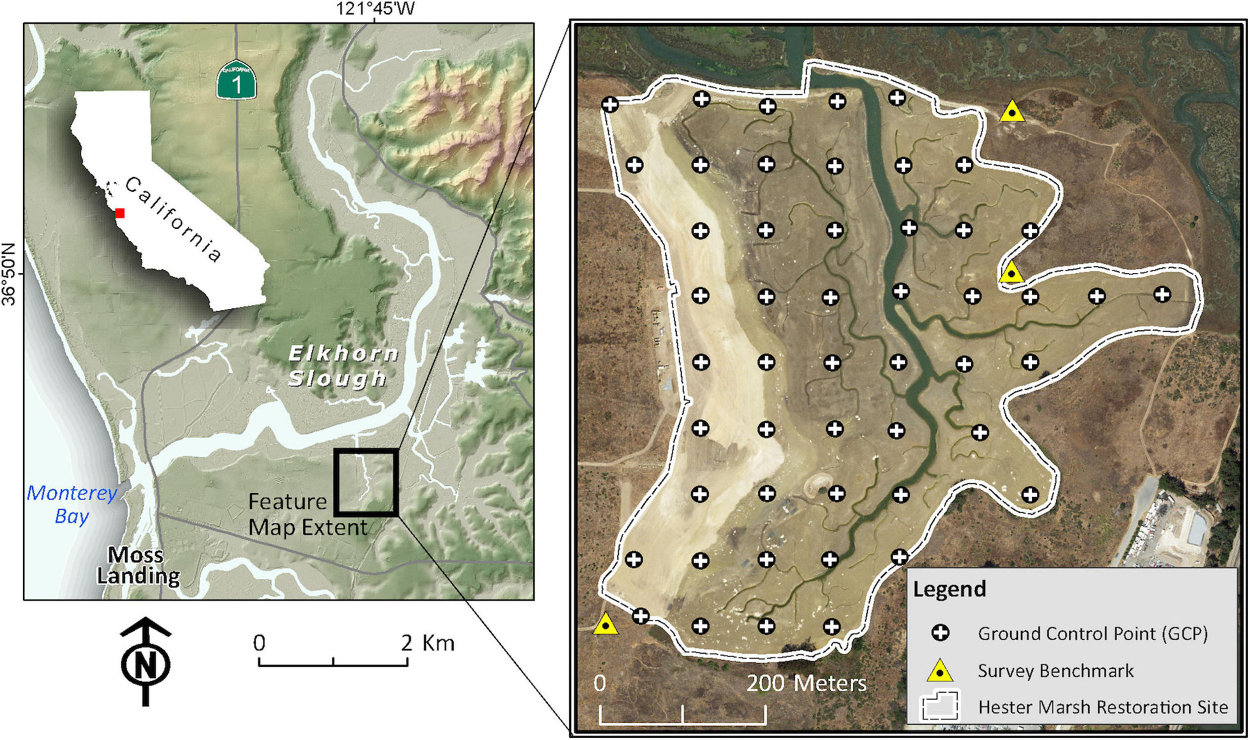
Figure 1. Map of the Hester Marsh restoration site in Elkhorn Slough, an estuary in Central California, United States. A grid of ground control points (GCPs) was established for linking UAV imagery to known locations on the ground. Elevations were surveyed at GCPs and referenced to survey benchmarks to create digital elevation models.
In 2004, the Elkhorn Slough National Estuarine Research Reserve (ESNERR) initiated the Tidal Wetland Program, an ecosystem-based management initiative, to address rapid changes in the estuary. The result of the decision-making process, which involved input from numerous stakeholders, was prioritization of marsh restoration (Wasson et al., 2015). ESNERR completed construction on a 25-hectare restoration project at Hester Marsh on the southern side of Elkhorn Slough in 2018 (Figure 1). Tidal exchange was cut off during the construction period of restoration and resumed when construction ended on August 8, 2018. Construction activities involved approximately 250,000 cubic yards of soil addition on a degraded and subsided marsh, which had converted mostly to unvegetated mudflat following human impacts such as diking and draining. Most of the soil used to elevate the marsh plain originated from an adjacent hillside that was formerly used for agriculture, was scraped during construction to provide soil, and is being restored to native grassland. The largest tidal creeks were left intact and secondary and tertiary creeks were excavated to resemble the historical creek network following soil addition.
Objectives for the restoration project addressed elements including marsh plain elevation, tidal creeks, and the marsh community. The construction target for initial elevation was 1.95 m NAVD88, near the upper limit of marsh plant distributions in Elkhorn Slough, and the marsh plain was expected to settle over time to a long-term target elevation of 1.89 m NAVD88. While some natural changes and minor developments to the tidal creek network were expected, main objectives for creeks were to mimic natural drainage patterns and limit bank erosion. High vegetation cover was another key objective, representing development of a healthy marsh community (Fountain et al., 2020). The Hester Marsh restoration project provided an opportunity for pilot testing of UAV methods for monitoring to evaluate progress toward these goals.
In October 2015, Tombolo Mapping Lab & Center for Habitat Studies at Moss Landing Marine Labs used a fixed-wing UAV (E384; Event 38 Unmanned Systems, Inc., Richfield, OH, United States) with a Canon SX260 HS 12-megapixel camera (Canon Inc., Tokyo, Japan) to collect aerial imagery at the study site. For all flights during and after site construction, we collected imagery with a DJI Phantom 4 Pro quadcopter (SZ DJI Technology Co., Ltd., Shenzhen, China) equipped with a 20-megapixel camera that collects visible spectrum (RGB) data. The quadcopter also carries a near infrared (NIR) and red-edge sensor (Double 4k sensor, Sentera Inc., Minneapolis, MN, United States), but use of these data was limited to testing of vegetation monitoring methods, where inclusion of NIR data was evaluated for one flight.
We created digital elevation models (DEMs) to monitor topography using UAV-collected photos and field-surveyed GCPs. The DEMs we used throughout our monitoring were digital surface models (DSMs), which by nature represent the elevation of the surface and thus, where there is dense vegetation or other features, the top of those features (Cruzan et al., 2016). We did not expect the use of DSMs to be an issue for our topography monitoring, as vegetation was absent or minimal in most of our imagery.
In order to determine the optimal flight altitude coupled with the minimum number of GCPs that maximized the accuracy of the results, we conducted a GCP density experiment involving a series of flights over an area of roughly 6.25 hectares within the restoration site. We compared vertical accuracy of DEMs created with varying densities of GCPs (0 – 6.4 GCPs/ha) and collected imagery at four flight altitudes (50 m, 75 m, 100 m, and 116 m; Table 1), resulting in a total of 34 DEMs that were assessed for accuracy. We encountered processing issues for the 75 m imagery georeferenced with 0 GCPs and 2 GCPs per hectare, so excluded these from our analysis. We sought to determine the threshold above which increased GCP density did not lead to notable decrease in root mean squared error in the vertical direction (RMSE; Coveney and Roberts, 2017).
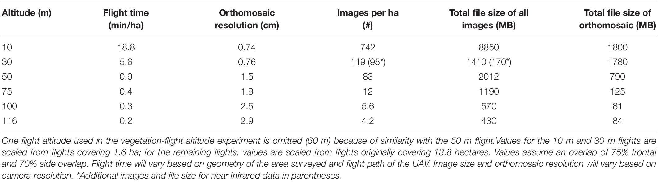
Table 1. General information for UAV flights conducted at six different altitudes for the GCP density and vegetation-flight altitude experiments.
The test site was a portion of the restoration site that had recently been filled with upland soils, creating a mostly level and unvegetated patch of ground. Using ArcGIS (v. 10.3; Esri, Redlands, CA, United States), we established a “fishnet” grid of 40 points spaced approximately 35 – 50 m apart. We created forty GCPs using numbered, 12” round white and black five-gallon bucket lids, and deployed them in the field using a handheld Trimble GPS. We used a Trimble VX TLS (Trimble Navigation, Sunnyvale, CA, United States) to survey the horizontal and vertical position of each GCP, as well as 66 randomly spaced check points. Elevation was referenced to a local tidal benchmark (NAVD88). Vertical accuracy of the TLS survey data was approximately ± 1 cm, slightly better than expected from a traditional RTK survey which would also require use of a base station, rover, and radio antenna.
Imagery was collected with 75% frontal and 65% side overlap, the default in our flight planning software (DroneDeploy, San Francisco, CA, United States). We used Agisoft Metashape software (v. 1.6.3 10732; Agisoft LLC, St. Petersburg, Russia) to create orthomosaics and digital elevation models (DEMs) using Structure from Motion (SfM) principles. We used Agisoft’s batch processing function to build orthomosaics and DEMs from the images collected during each UAV flight (details in Supplementary Table 1). All images (58 – 274 per flight) were georeferenced with coordinate system WGS84 / UTM zone 10N. Photos were manually georeferenced with GCPs in Agisoft Metashape. We used these basic processing steps to produce all DEMs and orthomosaics described throughout this study (except for the vegetation-flight altitude experiment), using the GCP density identified through this experiment for all flights beginning in August 2018. To evaluate vertical accuracy, check point elevations collected in the field were used to extract elevations from the DEMs using ArcMap Spatial Analyst. We calculated the difference between the field-surveyed check point elevations and DEM elevations and computed the accuracy (measured as RMSE) for the 34 resulting DEMs. We also evaluated horizontal accuracy (RMSE) for select images by creating points representing the center locations of the GCPs visible in orthoimagery and used the Point Distance tool to calculate the horizontal offset from the TLS-derived positions. We calculated additional error metrics for the highest-resolution (50 m altitude) imagery.
We compared three variations of UAV topography data collection with traditional field methods – TLS and SETs – and with airborne LIDAR to evaluate relative benefits of different approaches. The three UAV methods we evaluated used different georeferencing techniques: 1) UAV with onboard uncorrected global navigation satellite systems (GNSS), referred to as UAV–GNSS; 2) UAV with GCPs, surveyed using real-time kinematic (RTK) positioning and evaluated using independent check points, referred to as UAV–GCP; and 3) UAV with post-processed kinematic (PPK) dual-frequency differential GNSS corrected using either a base station in the study area or a nearby CORS station (Continuously Operating Reference Station), referred to as UAV–PPK. We compared these methods based on spatial coverage, vertical (RMSEz) and horizontal (RMSEr) accuracy, initial cost investment, training requirements, time and personnel required for one survey, and temporal and spatial resolution. Training requirements are categorized as “Low” (no prior experience or certification needed), “Moderate” (some experience with the equipment and specific licensing), or “High” (extensive field experience with the equipment and specific licensing).
We report horizontal and vertical error values for the UAV–GNSS and UAV–GCP methods from our GCP density experiment. The values for the UAV–GCP method are based on the GCP density and flight altitude we selected as optimal through this experiment. For the UAV–GNSS method, we used horizontal and vertical error values from imagery collected at that same flight altitude, not georeferenced using any GCPs. The horizontal error value for the UAV–PPK method is from a study comparing UAV georeferencing techniques (Padró et al., 2019b). The authors report horizontal accuracy as error in the radial direction, which includes both X and Y error. Suggested spatial resolution is the DEM cell size we believe to be appropriate based on horizontal error values.
To estimate costs of the different UAV approaches, we considered the aircraft and key accessories, software, and ground control points and equipment to survey them (for details see Supplementary Table 2). Although one-time rental fees may greatly reduce the investment costs of UAV equipment, the need for repeat surveys for long-term monitoring makes purchasing equipment less costly. To estimate time requirements for the UAV methods, we considered mission preparation (Haskins, 2020), the flight itself, GCP layout and surveying, and post-processing (details in Supplementary Table 3). Passive computer processing time to create the orthomosaics and DEMs is not included in the table since it will vary considerably depending on computer hardware, processing software and specific processing parameters. All UAV flight times assume a 65 m flight altitude covering a 42 ha area with the Phantom 4 Pro quadcopter. Spatial coverage will vary significantly based on the UAV type, total available battery life, flight altitude, and ability to maintain line of sight. The value we report is based on our experience with the Phantom 4 Pro quadcopter, flying at an altitude of 65 m with three batteries available and is intended to give the reader a reference.
To determine TLS error values for comparison with other methods, we identified horizontal and vertical errors during repetitive Trimble VX Spatial Station setups that measured coordinates of established control points. Suggested spatial resolution is based on accuracy of digital surface models created from surveyed point clouds, which is directly related to point spacing. Initial investment cost is based on a 2020 estimate of purchasing the survey equipment new and includes the spatial station, survey controller, batteries, tripods, target reflectors, survey rod, and carrying cases. Daily rental costs, alternatively, may range between $300 and $600. Spatial coverage assumes a survey area measuring 80 m × 80 m with two or more station setups and a point cloud spacing of approximately 10 cm. Time and personnel requirements include a minimum of one survey technician for a daily survey of an area this size and for post-processing.
Accuracy values for SET monitoring are based on the fact that SET pins measure the exact same location on the marsh surface during each successive survey. Unlike the other survey methods that produce dense point clouds and DSMs, SETs are generally limited to a few locations in a marsh and are not intended to be used for broad spatial analyses. Therefore, both spatial resolution and spatial coverage represent the approximate total area covered by a single SET. Initial investment cost includes the cost of one deep rod SET table, fiberglass pins, stainless steel receiver, and approximately 12 meters of stainless steel rods used to establish the SET monument. Time required for a survey includes reading the SET pins and recording measurements, and does not include initial setup time of the SET, which may take several additional hours.
Reported LIDAR accuracy can vary widely based on different instrumentation and landscape variations. We include vertical accuracy values (RMSEz) for an airborne LIDAR-derived DEM in a marsh setting, reported by Hladik and Alber (2012). Horizontal accuracy is based on horizontal point spacing for airborne LIDAR reported by Beland et al. (2019), and spatial resolution is based on this point spacing and general convention. Initial investment cost is an estimated value for acquisition and processing of airborne LIDAR data by a professional LIDAR contractor, and covering an area up to 1000 ha in size (Beland et al., 2019). While airborne LIDAR can cover a larger area, this will result in increased cost. Temporal resolution will vary according to location, and is an approximation based on local (Central California coast) LIDAR surveys. We assumed that LIDAR data would be collected by an external party and downloaded in a ready-to-use format by the user, so we did not include time or personnel requirements for this method.
We conducted a second experiment to determine the optimal flight altitude for fine-scale vegetation monitoring. For this vegetation-flight altitude experiment, we examined the accuracy of vegetation cover classification, and the visibility of plants of different sizes, from orthomosaics collected at 10 m, 30 m, and 60 m flight altitudes covering a one-hectare area (Table 1). One orthomosaic at each altitude included visible spectrum (RGB) data only, while an additional orthomosaic at 30 m altitude also included near-infrared (NIR) data. All imagery was collected on May 29, 2019. We used red 12” round five-gallon bucket lids to mark plants for visibility assessment, mark plots for percent cover analysis, and georeference orthomosaics. Orthomosaics were stitched by and downloaded from DroneDeploy and georeferenced in ArcGIS (v. 10.7).
To determine the visibility of different sizes of plants in imagery collected at different flight altitudes, we marked 60 plants by placing bucket lids next to them and measured each plant in the field. We marked 20 plants in each of three size classes based on their longest diameter (<10 cm, 10 – 20 cm, and 20 – 50 cm). Half of all plants in each size class were Salicornia pacifica (pickleweed, the dominant marsh plant) and half were Spergularia marina (a common early marsh plain colonist). We viewed each marked location in true color RGB imagery for each flight altitude in ArcGIS and considered a plant “visible” if it could be distinguished from the background and identified as a plant. We did not evaluate NIR imagery in this portion of the vegetation-flight altitude experiment due to lower resolution of the NIR camera.
To evaluate the accuracy of vegetation cover estimates from classified UAV imagery, we measured percent cover at 24 plots in the field, classified each of the four orthomosaics (10 m RGB, 30 m RGB, 30 m RGBNIR, 60 m RGB) into vegetated and unvegetated areas, and compared the classified vegetation cover to field-measured cover in those plots. Each plot covered one square meter, grouped into six larger 2 m × 2 m plots. We chose plot locations that represented a range of vegetation cover values and included both of the main vegetation species present, Salicornia and Spergularia. We surveyed cover in the field by placing a one-square-meter gridded quadrat over each plot. We assessed ground cover at intercepts within the grid by recording all vegetation species, or bare ground, touched by a metal rod when dropped at each intercept. To calculate percent cover, we totaled the number of intercept “hits” for each species or bare ground within the plot, divided by total intercepts surveyed in the plot and multiplied by 100. There were no intercepts where both plant species were encountered, so overall vegetation cover in a plot was the sum of Salicornia and Spergularia cover. Number of intercepts surveyed per plot varied between 16 and 25 because we collected data along the edges of some quadrats. We weighted our analysis to account for these unequal intercept numbers.
We classified imagery in ArcGIS Pro (v. 2.3) in order to calculate UAV-based estimates of vegetation cover. We experimented with both pixel-based and object-based classification methods, but present results using pixel-based classification with a maximum likelihood classifier, which we found to be the most consistent method for our imagery. We updated training polygons as needed to optimize each classification, until making additional changes to the set of training samples only resulted in minor changes in the final classified image. We used a total of nine classes in each classification, representing the two vegetation species, varying shades of mud, and the red bucket lids used for marking. However, because none of our classifications were able to distinguish between vegetation species accurately, we evaluated accuracy of overall vegetation cover only.
We used a weighted Nash-Sutcliffe Efficiency (NSE) coefficient to measure how close classified vegetation cover was to field-measured vegetation cover in each plot. To calculate classified vegetation cover, we tabulated the area of each class in each of the 24 plots using ArcGIS tools, summed the area covered by Salicornia and Spergularia, divided the sum by the total quadrat area, and multiplied by 100. The weighted NSE equation is as follows:
where n is the number of sampled plots, E is estimated cover from classified imagery, M is measured cover from the field survey, and W is the number of intercept sampling points (weight). NSE is a normalized coefficient that determines how well the relationship between estimated and measured data fits the 1:1 line (Nash and Sutcliffe, 1970; Trescott and Park, 2013). We computed a weighted NSE to account for the different numbers of sampling points in each plot.
We collected UAV imagery during multiple stages of the restoration process. During construction, we collected and reviewed UAV imagery to monitor progress and coordinate with contractors. Flights were conducted approximately monthly, typically at an altitude of 60 m and sometimes up to 100 m. Following construction, we used UAV imagery to monitor revegetation. We conducted image classification to estimate vegetation cover across the entire site and investigated the patterns of vegetation development by examining classified vegetation cover in relation to elevation, a key factor structuring marsh vegetation communities (Zedler et al., 1999).
Our main analysis of new vegetation relied on UAV imagery collected in October 2019, using the flight altitude we determined to be optimal in our vegetation-flight altitude experiment. We classified the imagery into vegetated and unvegetated areas using a pixel-based maximum likelihood approach in ArcGIS Pro (v. 2.3). We evaluated accuracy of the classification by creating a confusion matrix in ArcGIS to compare how well the classification matched a visual assessment of the high-resolution orthomosaic at 99 points (56 vegetated and 43 unvegetated points). We computed the true skill statistic (TSS), a metric based on the true positive and true negative rates for each class taken from the confusion matrix, to represent classification accuracy (Allouche et al., 2006). We examined classified vegetation cover in relation to elevation data collected with UAV to determine whether there was an elevation range that was particularly favorable for new colonization. We only examined classified vegetation cover at elevations < 2.0 m to exclude most upland vegetation.
We used UAV-generated DEMs to monitor changes in topography over various time periods during restoration (Table 2). To determine whether UAV data are appropriate for calculating earthwork volume (the volume of soil moved during construction), we calculated the change in soil volume using UAV-derived DEMs collected before (October 2015) and after (June 2018) construction, and compared this value to the earthwork volume determined by professional surveyors.
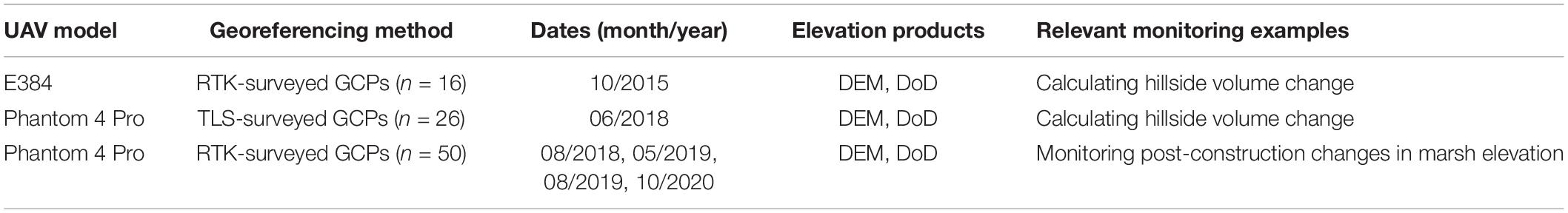
Table 2. Dates and basic methods for UAV-derived elevation products.
Because the pre-construction DEM (DSM) included areas with tall weeds, we corrected for vegetation-related errors by calculating the difference in elevation measurements between the 2015 DEM and a 2014 TLS field survey. The TLS survey was conducted using a Trimble VX Spatial Station at 302 points, with elevations referenced to local NOAA tidal benchmarks (vertical accuracy approximately ± 1 cm). We multiplied the mean elevation difference by the size of the hillside area to estimate the total vegetation-related error in the DEM. Vegetation error was not an issue in the post-restoration imagery because the area was bare following soil scraping. We subtracted the 2018 DEM from the 2015 DEM to create a DEM of Difference (DoD; a process known as DEM differencing) using ArcGIS raster calculator. We summed the difference values in each cell of the scraped area, and multiplied this sum by the cell size to calculate the uncorrected volume change. Subtracting the vegetation error from this value resulted in the actual soil volume change. We compared our value for earthwork volume with a value determined by professional surveyors, who conducted RTK field surveys at over 200 points on the hillside area before and after construction and calculated volume change in AutoCAD software.
After construction, we established a network of GCPs based on results of our GCP density experiment and continued to track topography changes using UAV DEMs and DoDs (Table 2). We also created a baseline DEM representing Day 0 that assumes a consistent elevation value of 1.95 m for all pixels, prior to the first post-construction UAV survey. We corroborated this assumption using the surveyors’ post-construction RTK survey at 310 points on the marsh plain. We examined topographic changes on the marsh plain and in tidal creeks using DEM differencing. We also used UAV data to evaluate the effectiveness of a bank stabilization method to minimize erosion. During construction, bay mud was dug up from the old marsh plain using a long reach excavator and compacted on the west bank of the main channel at the Hester restoration site to create a firm channel edge to reduce bank erosion. We examined DoDs and extracted vertical profiles from UAV DEMs to compare changes on the stabilized bank with the non-stabilized bank on the other side of the main channel.
Our GCP density experiment revealed that both GCP density and flight altitude had an effect on DEM accuracy, though GCP density drove most variation in accuracy. Accuracy was lowest (RMSE highest) at the lowest GCP density we tested for all flight altitudes (0 GCPs per hectare; Figure 2). Accuracy increased sharply with initial increases in GCP density, but changed very little once GCP density increased beyond 2.1 GCPs per hectare for all flight altitudes (accuracy metrics for 50 m flight in Table 3). We selected a density of 1.9 GCPs per hectare (50 total GCPs for our site) for our repeated monitoring to maximize accuracy while minimizing the time required for repeated GCP surveys. We initially used a flight altitude of 60 m, which required a relatively short flight time (45 min to cover 42 ha), but later adjusted flight altitude to 30 m based on our vegetation-flight altitude experiment.
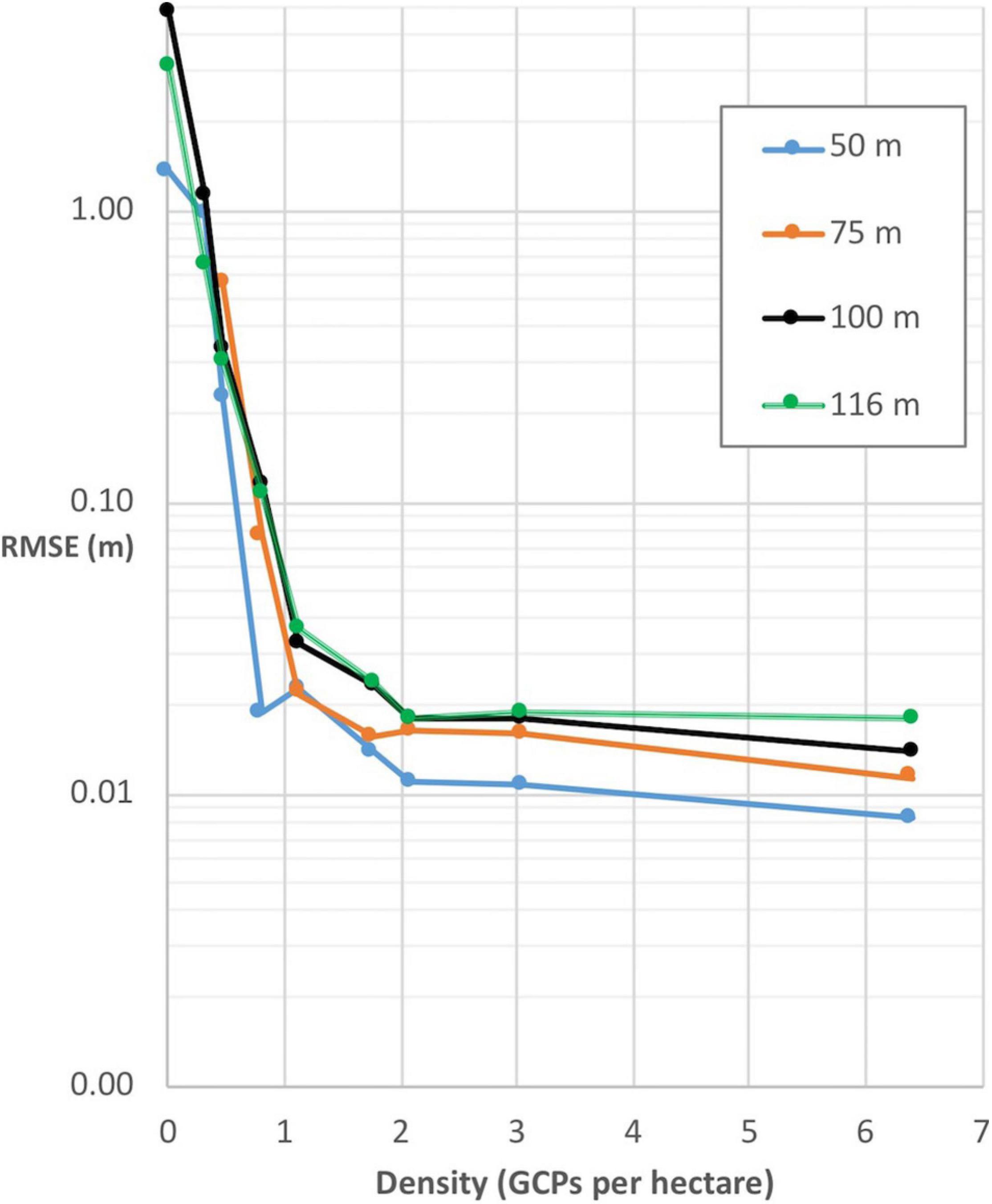
Figure 2. Relationship between vertical DEM error (measured as RMSE) and GCP density, plotted for data collected at four different flight altitudes.
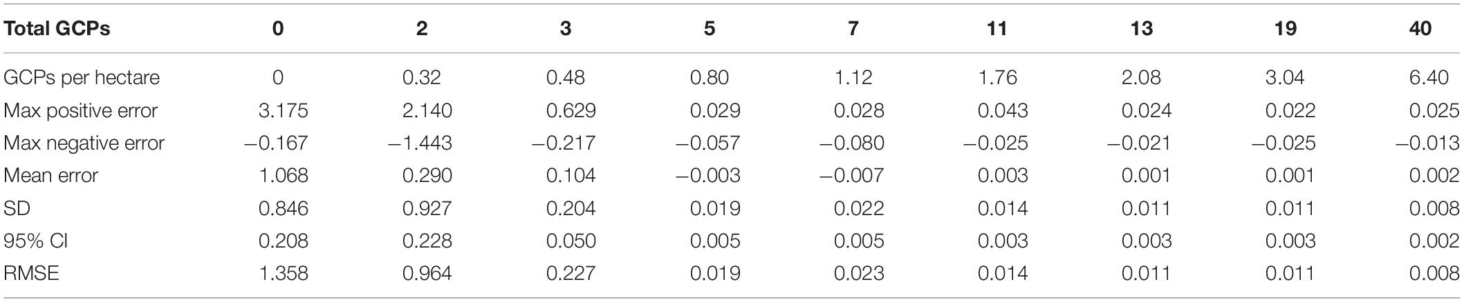
Table 3. DEM vertical error for imagery collected at 50 m altitude over a 6.25-hectare area. All error values are in meters.
We found substantial variation in accuracy and time requirements within the suite of UAV methods we compared, as well as variation in many parameters among UAV and the other topography monitoring methods (TLS, SET, and airborne LIDAR; Table 4). Coverage varied from under one hectare with both field-based methods to up to 1000 hectares with LIDAR, with all UAV methods covering a maximum of 42 hectares based on our selected flight altitude (65 m) and battery constraints (three batteries). We did not compare fixed-wing drones here, which typically offer better flight efficiency and maximum coverage (Johnston, 2019).
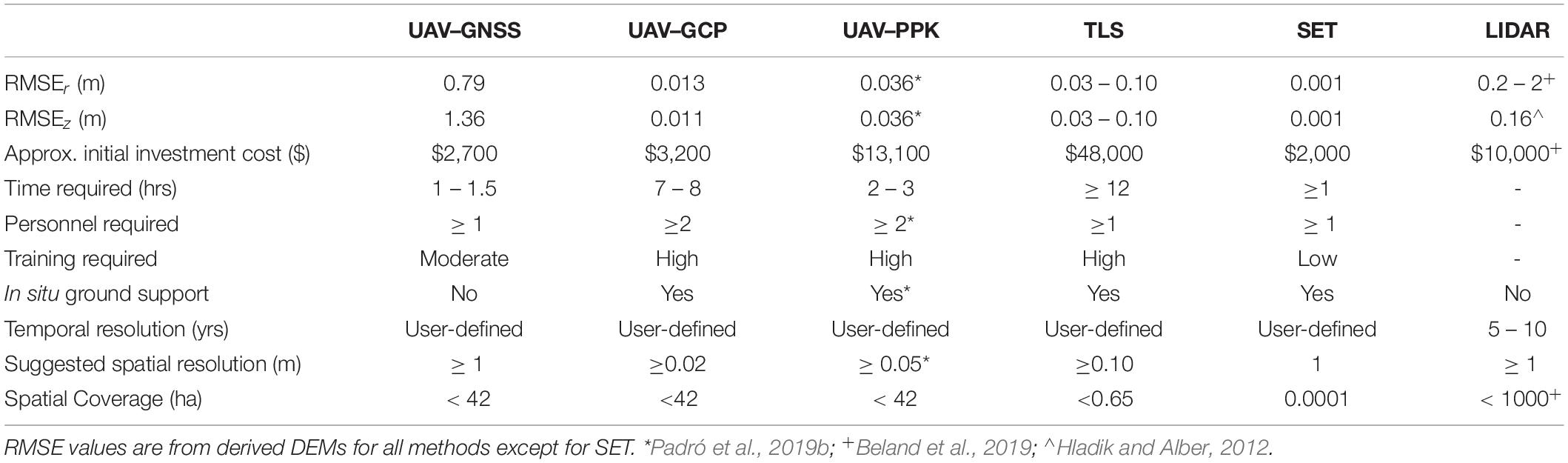
Table 4. Comparison of different topography data collection methods, including UAV with onboard uncorrected GNSS (UAV–GNSS), UAV georeferenced using 50 surveyed GCPs (UAV–GCP), UAV equipped with PPK (UAV–PPK), terrestrial laser scanning (TLS), surface elevation table (SET), and airborne LIDAR.
Horizontal error (RMSEr) was 10 cm or less for all methods except UAV–GNSS and LIDAR, indicating that those two methods should only be used for coarser analyses. While SET horizontal error is minimal (1 mm), having only one or a few SETs results in low spatial resolution and coverage. Although TLS offsets may also be very low (<1 cm vertical and horizontal), DEMs created from surveyed point clouds will produce larger errors (5 – 10 cm vertical and horizontal) that are directly related to the point spacing. For this reason, we suggest a spatial resolution of a minimum of 10 cm for most TLS-derived DEMs. Vertical error values (RMSEz) suggest that neither UAV–GNSS (1.4 m RMSE) nor LIDAR (0.16 m RMSE) would be sufficiently accurate for detecting the fine-scale changes valuable for marsh restoration monitoring. UAV–GCP, UAV–PPK, and SET are the most appropriate methods for this type of monitoring based on vertical error.
TLS was by far the most expensive method, whereas all other methods required an initial investment cost of approximately $13,000 or less. TLS involved the greatest time requirement, despite covering only a relatively small area. All UAV methods required less time to cover a much larger area, though time for UAV–GCP and UAV–PPK methods will vary depending on whether GCPs are permanently deployed or require removal after placement on the day of flight. While nearly all methods can collect data on a user-defined schedule, LIDAR may only be available every 5 – 10 years.
Our vegetation-flight altitude experiment revealed an expected decrease in image resolution (increase in pixel size) with increasing flight altitude (Table 1). While individual plants were very well-defined in imagery collected at 10 m altitude, plants appeared blurrier and harder to identify in imagery collected at 60 m altitude (Figure 3). Plant visibility increased with decreasing flight altitude for all size classes (Table 5). However, we were not able to detect most small plants in UAV imagery regardless of flight altitude. Plant detection was particularly difficult in areas where the substrate was more heterogeneous (dark cracks in mud, or pockets of darker mud).

Figure 3. UAV imagery, classified vegetation, and percent cover accuracy assessments for three different flight altitudes (10, 30, and 60 m). Visible spectrum (RGB) imagery is shown in true color, while the imagery including visible and near-infrared bands (RGBNIR) is shown in false color. Accuracy was assessed by comparing percent cover of classified vegetation with field-measured cover in 24 plots and calculating the Nash-Sutcliffe Efficiency (NSE) coefficient, which measures closeness to the 1:1 (dashed) line.
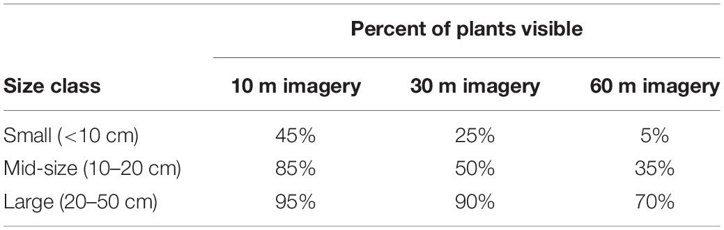
Table 5. Visibility of plants in imagery collected at different flight altitudes. Plants were grouped into size classes based on their longest diameter.
Accuracy of vegetation cover estimates based on image classification decreased with increasing flight altitude for the RGB imagery (Figure 3). While all four classified images represented the vegetated and unvegetated areas fairly well, the higher-altitude (60 m) flight performed the poorest in accuracy tests (NSE = 0.63) and classification of this imagery failed to capture many small plants (Figure 3). Classification of the imagery that included RGB and NIR data was best (NSE = 0.74) despite being collected at intermediate flight altitude (30 m), followed by 10 m RGB imagery (NSE = 0.71) and 30 m RGB imagery (NSE = 0.69). Based on these results, we mapped vegetation across the entire site with a 30 m altitude flight in October 2019 because we deemed the improvements in plant visibility and vegetation cover accuracy over the 60 m imagery to be worth the extra flight time and battery requirements. The time required to fly at 10 m altitude made this altitude infeasible for surveying the whole site (Table 1).
We used UAV imagery throughout the course of the restoration project to communicate with various audiences, track construction progress, and assess restoration success. Imagery from before construction showed the degraded marsh, which was mostly unvegetated mudflat covered in algal wrack with a relatively small amount of healthy marsh vegetation on the edges (Figure 4A). Immediately after construction, imagery showed a bare marsh plain free of algal wrack (Figure 4B). During construction, managers used UAV imagery to view the entire site and evaluate whether progress matched intended plans (Figure 5).
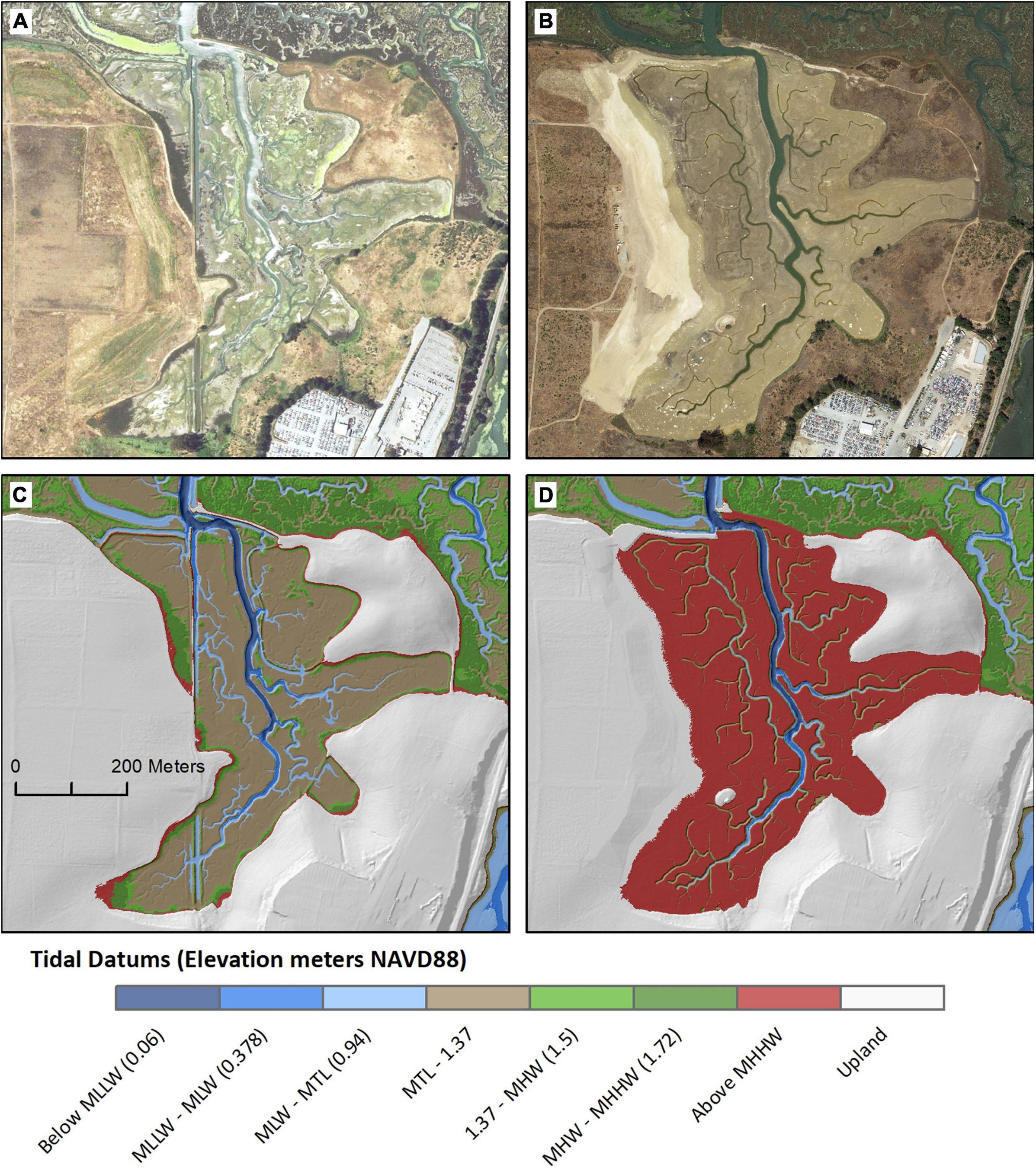
Figure 4. UAV-collected orthomosaics of Hester Marsh showing (A) the degraded marsh prior to construction in 2015, and (B) the initially bare marsh after construction was completed in 2018. UAV DEMs showing the change between (C) pre-construction elevation in 2015, and (D) post-construction elevation in 2018.

Figure 5. Maps collected during construction (June 2018) and at the end of construction (August 2018) showing a narrow peninsula that was constructed following old creek network designs, and then changed to reflect updated designs. We primarily used orthomosaics to monitor construction, but present DEMs here to make the change more easily visible. Note lower DEM resolution in the June 2018 imagery due to different processing technique with no GCPs.
Classification of imagery collected in October 2019, roughly a year after construction ended, revealed a total of 6.8% vegetation cover on the marsh plain and patchy patterns of new colonization that we explored in relation to microtopography (Figure 6A). Graphing classified vegetation cover and topography data from UAV DEMs revealed greatest vegetation cover at the highest elevations that we examined (1.95 – 2.00 m NAVD88; king tide line is around 2.15 m NAVD88), moderate cover at low elevations (1.75 – 1.80 m), and lowest vegetation cover at mid-elevations (1.85 – 1.90 m; Figure 6B).
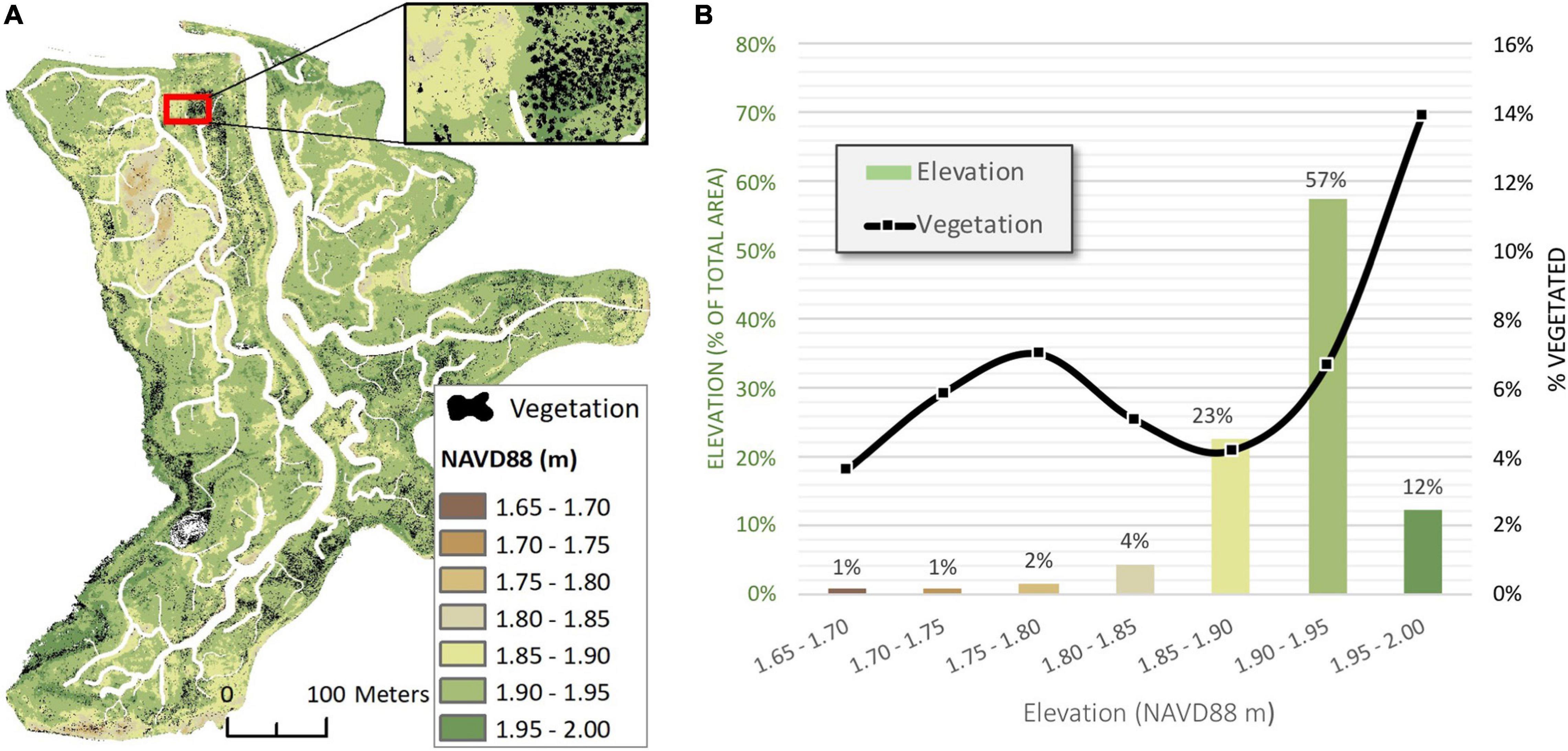
Figure 6. (A) Map of classified vegetation on top of an August 2018 DEM showing elevation in 5 cm increments. (B) Percent of total area (histogram) and percent vegetated area (line) in each elevation bin. Percent vegetated area is the area of classified vegetation in an elevation bin out of the total area in that bin.
In addition to imagery, UAV-derived DEMs were also used for communications and outreach. A 2015 DEM clearly showed how subsided the pre-restoration marsh plain was in comparison to healthy nearby marsh (Figure 4C). Most of the area was between mean tide level (MTL) and mean high water (MHW; 1.50 m NAVD88 according to Van Dyke, 2012), an elevation range that is inundated too frequently to support the dominant marsh vegetation, Salicornia (Larson, 2001). In contrast, the 2018 DEM collected after construction ended showed how high the new marsh plain was in comparison to the former subsided marsh plain and the nearby healthy marsh, with the entire restored marsh plain above mean higher high water (MHHW; 1.72 m NAVD88 in Van Dyke, 2012; Figure 4D).
DEM differencing to measure earthwork volume clearly highlighted the upland area of negative elevation change where soil was removed during construction (Figure 7). Our UAV-derived estimate of earthwork volume based on the DEM of Difference (DoD) corrected for vegetation-related error was 165,312 m3, which was very similar to the surveyors’ estimate of 166,673 m3. Before correcting for vegetation, DEM differencing indicated a volume change of 178,604 m3. The 2014 TLS survey used to correct for vegetation recorded similar elevations to the 2015 DEM in areas lacking ground vegetation (68 of 302 survey points had a difference of < 3 cm between TLS and DEM data). However, the mean difference between TLS and DEM elevations was 14 cm, with greater elevations in the DEM in areas of dense vegetation. We estimated the error due to vegetation to be 13,292 m3.
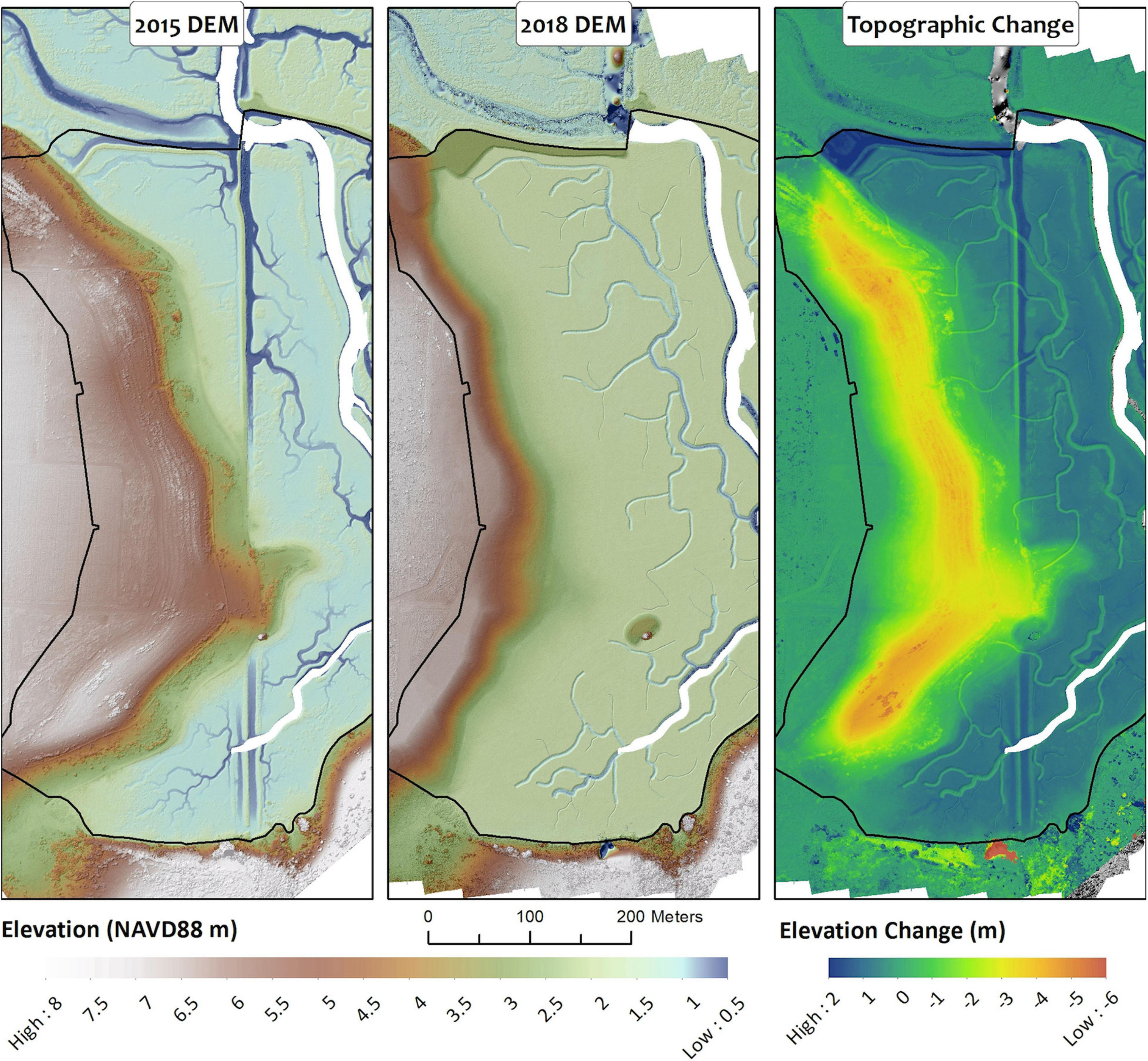
Figure 7. Maps showing elevation change on the western side of the restoration site, where soil was scraped from the hillside to elevate the marsh plain. A DEM of Difference (right) represents topographic change between pre-construction (2015 DEM, left) and post-construction (2018 DEM, middle) and was used to calculate the volume of soil moved from the hillside during construction.
Post-construction topography monitoring of the marsh plain with UAV revealed that the marsh plain elevation target was met and maintained, with the expected relatively slight subsidence. The RTK field survey corroborated the assumption of a consistent 1.95 m elevation for the Day 0 DEM, showing a mean elevation of 1.951 m at 310 points. The first post-construction UAV DEM collected at the Hester Marsh restoration site (21 days after construction ended) indicated a mean elevation of 1.915 m on the marsh plain, which was between the initial target elevation of 1.95 m and the long-term target elevation of 1.89 m.
DEM differencing revealed that there was < 0.05 m of elevation change across most of the marsh plain, with some spatial variation including greater subsidence in some areas and elevation gains in others (Figures 8A,B). Greater magnitude and area of negative elevation change in the first DoD (0 – 21 days following the end of construction and return of tidal exchange; Figure 8A) indicates that most subsidence occurred over the first 3 weeks compared with the following 9 months (21 – 285 days; Figure 8B). This temporal trajectory of subsidence and spatial variation is also shown in the values extracted from DoDs at the field survey points. These data show a drop in mean elevation of about 3 cm over the first 21 days and little change thereafter (Figure 8D). Some areas show greater drops in elevation over that initial period, around 12 cm, while others show slighter and more gradual loss in elevation (Figure 8D).
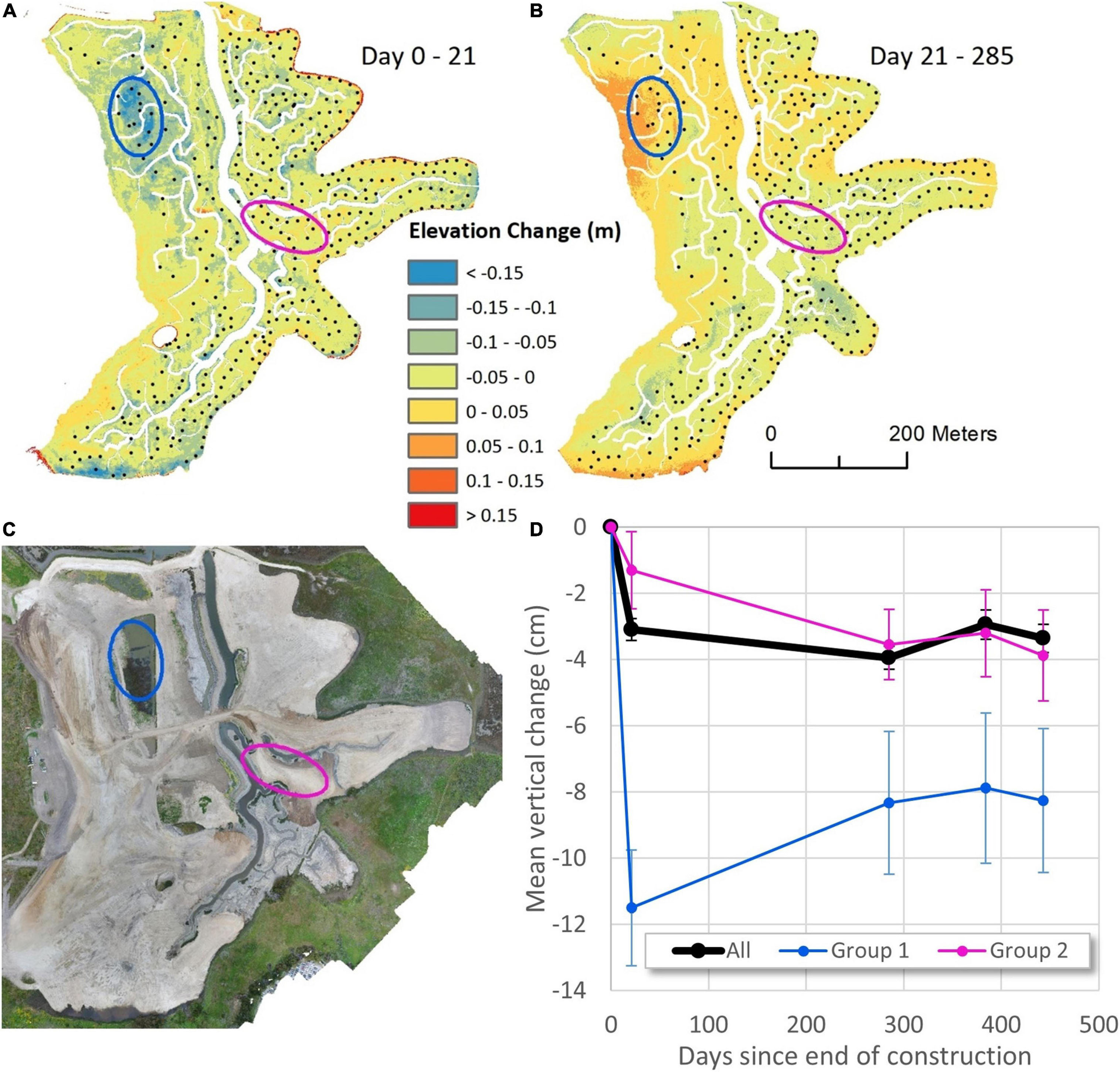
Figure 8. Spatial and temporal patterns of elevation change at Hester Marsh. (A) DoD showing elevation change in the first 21 days following construction, assuming a consistent Day 0 elevation of 1.95 m. Black points show locations of the RTK survey completed at the end of construction in 2018. (B) DoD showing elevation change between Day 21 and Day 285. (C) UAV orthomosaic captured in May 2018 showing an area where excess water was contained during construction (blue oval) and where soil was compacted early on as part of a construction vehicle route (fuchsia oval). (D) Mean difference in original RTK-surveyed elevations and elevation values extracted from four post-construction DEMs at those surveyed positions. The black line represents elevation change at all RTK-surveyed positions, blue line represents the subset of locations within the blue oval in all maps, and fuchsia line represents the subset of locations within the fuchsia oval in all maps.
Post-construction monitoring of creeks using UAV showed that the tidal creek network was developing, with limited bank erosion. A DoD representing vertical change that occurred between the first month following construction (August 2018) and the following year (October 2019) indicated deepening of smaller tidal creeks over time, particularly where they connect with larger creeks (Supplementary Figure 1). The DoD also shows development of new small creeks, with some limited erosion on the banks of the larger creeks. Some minor areas of positive elevation change in the DoD correspond to dense, large plants that colonized over the first year and are visible in October 2019 imagery.
Examining a DoD and elevation profiles of the main channel banks at different time points revealed differences in bank erosion between the stabilized and non-stabilized banks (Figures 9A–C). While the transects across the stabilized (west) bank edge showed similar or even slightly higher elevation profiles one year after construction (October 2019) compared with the initial profiles (August 2018), the transects across the non-stabilized (east) bank showed elevation loss on the non-stabilized bank edge. Orthomosaics and field observations suggest that the elevation increases may reflect vegetation colonization and growth (Figure 9A).
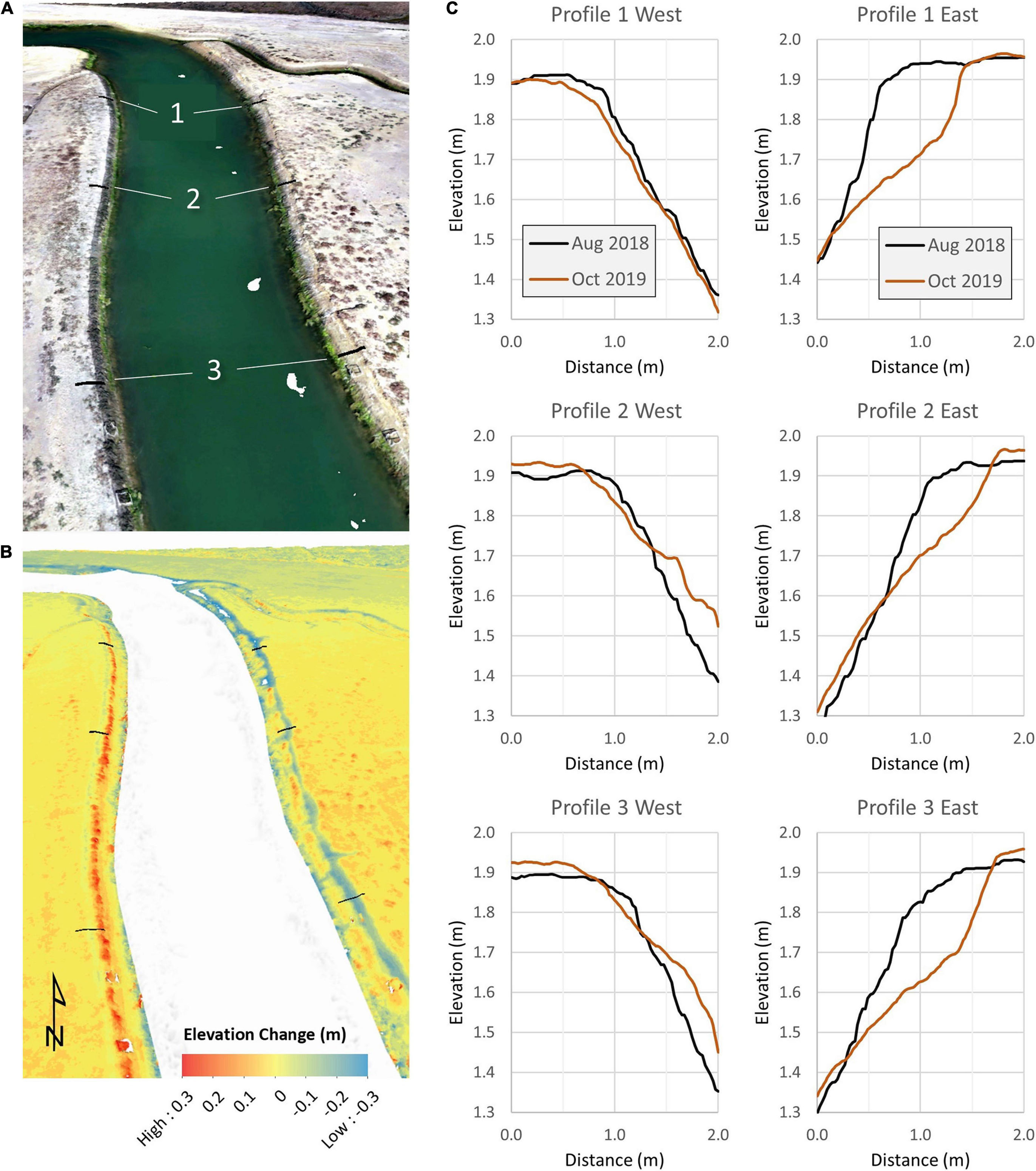
Figure 9. A portion of the Hester Marsh main channel shown in (A) an October 2019 orthomosaic, and (B) a DoD between August 2018 and October 2019. The west bank of the channel was reinforced with mud excavated from the former wetland; the east bank had no reinforcement. (C) Vertical profiles extracted from UAV DEMs were used to evaluate erosion of the main channel banks between August 2018 and October 2019.
We successfully developed and implemented methods for UAV monitoring of marsh restoration, and for creating products useful to restoration stakeholders. Below, we share methodological recommendations and illustrate the diversity of applications of UAV data in restoration monitoring. While we focus on our case study of a California tidal marsh restoration project, the general lessons learned can inform UAV-based restoration monitoring in a variety of other habitats.
Overall, the methods we developed were effective for monitoring elevation and vegetation at the scale and spatiotemporal resolution needed for our project, where detecting small changes in elevation over time, and evaluating colonization by small new plants was essential for monitoring restoration success. Our experiments evaluating different UAV methodologies resulted in several recommendations for monitoring topography and vegetation using UAV.
Our first recommendation is to explicitly plan for UAV monitoring before, during, and after restoration monitoring (Figure 10). While we developed our topography and vegetation monitoring methods during and after construction, others may find it optimal to determine these methods prior to construction. Surveying at reference sites may be an appropriate way to determine a specific protocol for monitoring ground cover and topography at the restoration site. An important benefit of determining how to make accurate DEMs early on, particularly in soil addition marsh restoration projects, is enabling creation of accurate pre-restoration topography maps. At our site, we conducted an earthmoving volume assessment that relied on a non-bare-earth DEM collected prior to restoration (Figure 7), and an accurate calculation of soil volume change required correcting for vegetation using a field survey. Carrying out pre-restoration flights for method development could also be valuable for determining limitations of using UAV in a given system, such as whether species of interest can be distinguished from each other and from the background substrate, and for identifying potential risks and hazards (Haskins, 2020).
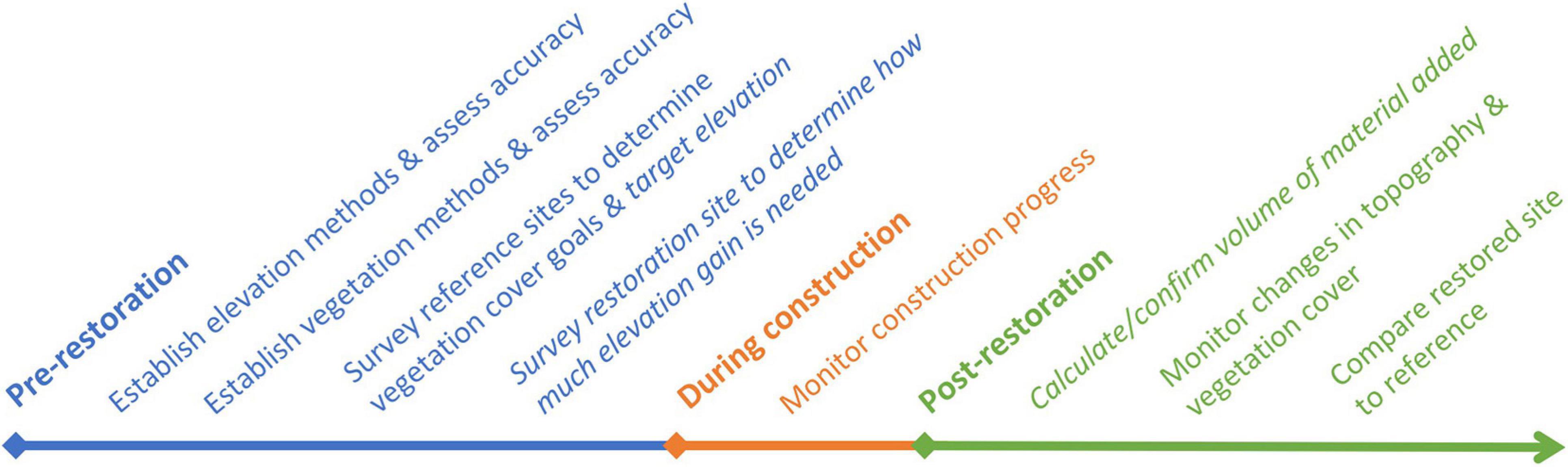
Figure 10. Recommendations for timing of UAV monitoring, generally applicable to all restoration (regular text) and specific to sediment/soil addition projects (italic text).
Secondly, we recommend that sites with similar fine-scale topography monitoring goals use a similar GCP density to the one we determined to be optimal in our experimentation. Our methods for topography monitoring generated highly accurate DEMs (1.1 cm RMSE) and can likely be applied to other sites of a similar size. We found that a GCP density of about 2 GCPs per hectare was ideal, and that increasing GCP density above that level would not result in substantially greater accuracy but would increase field survey time. Flight altitude did not have as strong an influence on DEM accuracy, so we initially flew at an altitude of 60 m, which enabled rapid data acquisition. We later reduced the flight altitude to 30 m in order to better capture recently colonized vegetation. Where vegetation became larger and denser, we noticed errors in the DEM because, as a DSM, it represented the top of the vegetation canopy in these areas rather than the ground (Supplementary Figure 1). One way to correct this is by incorporating additional processing steps to filter out vegetation from the DSM (for example, see Cunliffe et al., 2016). The methods we utilized to create DEMs could be valuable for other types of restoration, particularly when microtopographic variation is important to capture. While other studies may choose to use a similar approach to ours in terms of flight altitude and GCP density, researchers at sites of different sizes, or with different accuracy needs, may find it helpful to conduct an experiment similar to ours to determine their optimal methods.
Our third recommendation is to use UAV imagery to track revegetation of the restoration site, using the approach we successfully piloted for data collection, modified as needed for different habitats or sites of different size. At our site, a flight altitude of 30 m enabled sufficiently accurate calculation of vegetation cover compared with field measurements (NSE = 0.69 using RGB imagery), and subsequent exploration of the relationship between new vegetation cover and elevation. While we decided the longer flight time to collect imagery at 30 m altitude was worthwhile for detecting more individual plants and therefore minimizing the need for ground-truthing in the field, a 60 m flight altitude may be sufficient when most plants are larger and less sparse. Other studies comparing UAV flight altitude/image resolution for detecting and classifying small plants have also reported that accuracy increases with greater image resolution, collected at lower flight altitude, but this increase is sometimes marginal (Torres-Sánchez et al., 2014; Buters et al., 2019b). Others have also found that detection of small plants is easier on more homogenous substrates (Buters et al., 2019b), a conclusion that our findings support. We recommend collecting NIR data in addition to RGB data, which improved vegetation cover estimates in 30 m imagery (NSE = 0.74), but we had issues with either sensor capture or file management that prevented us from using NIR data in our classification of October 2019 imagery covering the entire restoration site. In projects that compare imagery between sites or dates, researchers should collect calibration images that capture a reflectance target before, during, and/or after each flight to calibrate imagery (Assmann et al., 2018).
To elaborate on the third recommendation above, we used image classification to estimate vegetation cover and examine spatial variation from UAV imagery, and suggest that others optimize the specific classification method based on their software and imagery. While the pixel-based maximum likelihood classification we used for UAV-based vegetation cover estimates was adequate for our purposes, many other classification options exist and could improve the accuracy of percent cover estimates. For example, object-based classification methods can incorporate additional factors such as shape and texture of distinct objects, which may be beneficial for distinguishing plants from mud (Dronova, 2015). While we were unable to distinguish between species in our classifications, this type of distinction might be possible with modifications to the data collection and/or classification method. For example, imagery can be collected during times of year when the species appear more different due to flowering or other phenological changes (Gilmore et al., 2008). Some studies also incorporate elevation data into image classification, which can help distinguish between similar-looking vegetation classes when they occupy different vertical zones (Sturdivant et al., 2017; Padró et al., 2019a). Our methods for UAV monitoring of new plants using image classification will work well on initially bare sites when vegetation is easily distinguished from the background, and separating different species or vegetation types is not critical. Given many site-specific factors in vegetation monitoring, the accuracy values we achieved in classifying vegetation cover may not translate to other systems and conducting test flights should be considered essential.
Determining an appropriate monitoring method is vital for ensuring that lessons are learned from restoration without exceeding limited budgets (Roegner et al., 2008). Our comparison of UAV with TLS, SET, and airborne LIDAR methods for topography monitoring, and our firsthand experience monitoring vegetation and topography at this site using both field and UAV methods, revealed some key benefits of UAV over field monitoring as well as a few drawbacks.
A clear benefit of UAV monitoring includes its capacity to generate high spatial resolution data across an entire site including hard-to-access areas. Our construction monitoring benefitted from the ease of monitoring areas with UAV that were not easily accessible on foot. For example, midway through the construction period, we detected a narrow, erosion-prone peninsula in the interior of the site that had been constructed according to an old creek network design (Figure 5). Rapid detection of this issue in UAV imagery enabled us to update construction in this area to shorten the peninsula. The comprehensive spatial coverage of UAV data was also valuable for detecting and analyzing spatial patterns, which field sampling could miss if not distributed well across the whole site. For example, field surveys of subsidence would provide an incomplete or misleading picture if coverage was too limited or certain key areas were missed (Figures 8A–D).
Customization of temporal resolution of data is another valuable attribute of UAV monitoring, enabling data collection to be easily tailored to monitoring needs and research questions (Easterday et al., 2019). Temporal resolution is least customizable for aerial or satellite data (e.g., LIDAR), and is customizable for field data but with spatial coverage limitations (Table 4). At our site, the ability to collect frequent topographic data with UAV enabled us to determine that most subsidence occurred in the first few weeks of tidal exchange (Figure 8D).
There are notable differences among UAV methods in cost and time efficiency as well as accuracy of products (Table 4). While two of three UAV methods were comparable in cost to SET monitoring (the cheapest topography monitoring method in our comparison), UAV–PPK involved greater initial investment cost. However, this industry has been evolving rapidly over the past decade, and costs for all UAV methods may continue to decline. Compared with UAV–GCP (the most accurate UAV method), UAV–PPK required less time for one survey and accuracy of this method was only slightly reduced. The most rapid and inexpensive UAV method (UAV–GNSS) was not accurate enough for our monitoring purposes. While UAV monitoring was more efficient than the field methods we use to regularly survey both topography and vegetation at our site, one notable drawback in comparison to many field methods is the lower level of detail captured in UAV data. Field survey time to collect both vegetation and topography data at our site required a minimum of 2.5 person-hours to fly the UAV (at 30 m altitude, covering the 25 ha site and adjacent areas) compared with 22 person-hours for field data collection (10 h for vegetation cover, 12 for elevation at 100 quadrats). Reduced detail was evident in our inability to distinguish between species, upland vs. marsh plants, or native vs. non-native plants in classification of UAV imagery. For elevation, we found our UAV DEMs to be highly accurate, but note that using SETs is more accurate by an order of magnitude (Table 4).
Another drawback of UAV as well as TLS monitoring is the moderate to high training required (Table 4). While SET monitoring can be accomplished with low training, all UAV methods require at least moderate training (some experience operating the equipment as well as a FAA 107 drone operator license) and the most accurate UAV methods have high training requirements. Because of the many different considerations when choosing a monitoring methodology, and the lack of a clear winner across all categories, monitoring decisions should be made based on anticipated applications of the data.
Tracking and communicating about restoration progress is critical for generating public support for restoration, meeting permitting and funding requirements, maintaining institutional support, making management changes to improve outcomes, and informing decisions for future projects (McDonald et al., 2016). Aerial imagery is one powerful tool to accomplish these goals and maximize the benefits of restoration projects. Other restoration studies in a variety of habitats are beginning to use UAV, primarily for post-restoration vegetation cover monitoring (Knoth et al., 2013; Buters et al., 2019a; Padró et al., 2019a; Reis et al., 2019; Pérez et al., 2020). For restoration in more densely vegetated habitats, UAV-derived elevation data has also been used to monitor canopy structure (Zahawi et al., 2015). Other than vegetation monitoring, UAVs have also been found to be useful for monitoring geomorphic change and spatial patterns of erosion and aggradation in restoration of intermittent streams (Marteau et al., 2017). However, few prior studies using UAV at restoration sites focus on the early stages of restoration, which involves collecting data of sufficiently high spatial resolution to capture small, sparse plants and subtle variations in elevation.
We frequently relied on imagery collected using UAV to communicate with the broader community about the restoration project, including the public, funders, and other stakeholders (Figures 4A–D). Estuarine habitats are hard to access, so imagery helps to share progress of projects with the public, builds excitement for successes like seeing plants return, and helps generate support for marsh conservation and restoration. We used UAV imagery in many presentations about the restoration project, as well as in teacher training workshops illustrating how marsh restoration can enhance resilience to sea level rise by building new habitat at a high elevation in the tidal frame (Figure 4D). UAV products were also valuable for communicating with specific audiences like funders, to whom we reported whether goals were met on metrics including elevation, hydrology, and vegetation.
Monitoring was also valuable for informing adaptive management and planning for future restoration projects. During construction, rapid detection of the erosion-prone peninsula in UAV imagery enabled contractors to make changes while equipment was onsite, preventing potentially large future costs (Figure 5). Our UAV-based assessment of the volume of soil moved from the hillside onto the marsh plain during construction was used to verify the surveyor’s assessment and was a critical corroboration because earthwork volume is an important determinant of restoration construction costs (Figure 7). Accuracy of this UAV volume assessment method indicates that it can be used to estimate construction costs during planning of future projects, serve as an alternative to the more traditional field methods used by surveyors, or corroborate surveyors’ assessments.
Repeated topography monitoring following construction revealed some areas of subsidence (Figures 8A,B), where water was pooling and plants were not readily colonizing, some of which we were able to target for filling by contractors. Future analyses can take advantage of UAV-collected imagery and topography data to examine whether the spatial variation in subsidence is tied to previous land use or construction methods, such as areas that were used for containing excess water during construction (Figure 8C). Understanding how much subsidence occurred, and spatial patterns, enables managers to adjust the initial elevation and construction methods of future soil addition projects. The observed topography changes on a stabilized and non-stabilized bank suggested that bank stabilization not only successfully reduced erosion but also potentially promoted vegetation growth (Figures 9A–C). These findings led to implementation of bank stabilization on a larger scale in a new, adjacent marsh restoration area under construction in 2020.
Ultimately, tidal marsh restoration aims to create favorable conditions for redevelopment of the biotic community, including vegetation (Zedler, 2000a; Roegner et al., 2008). Monitoring revegetation using classified UAV imagery helped us understand factors that influence vegetation cover, such as microtopography (Figure 6), with the goal of preventing conditions that inhibit colonization at future sites. The applications we have described could be implemented in many different types of habitat restoration, supporting the critical communication of restoration progress with key stakeholders and ensuring knowledge is gained from restoration projects to inform both adaptive management and future planning (McDonald et al., 2016).
The datasets presented in this study can be found in online repositories. The names of the repository/repositories and accession number(s) can be found below: https://doi.org/10.6084/m9.figshare.c.5226785.v1 (Figshare).
AT created the first draft of the manuscript and literature review, and conducted the vegetation-flight altitude analysis. JH, CE, and FG conducted the topography method development, carried out repeated monitoring, and contributed most of the figures. MF and KW secured funding and provided oversight. All authors contributed to idea development, writing, and editing of the manuscript.
The Hester Marsh restoration project was coordinated by ESNERR’s Tidal Wetland Program and funded by grants from California Department of Water Resources (4600009727), California Department of Fish and Wildlife Greenhouse Gas Program (P1496007), California Coastal Conservancy (16-019), USFWS National Coastal Wetlands Conservation Program (16-019), Ocean Protection Council (P01-2-04), and the Wildlife Conservation Board (WC-1522SM) to the Elkhorn Slough Foundation on behalf of ESNERR. The UAV monitoring of Hester, including analyses and manuscript preparation, was funded in part by these sources as well as NOAA’s Office for Coastal Management (NA20NOS4200097, NA19NOS4200050, NA18NOS4200075, NA17NOS4200041, and NA16NOS4200073), and the NOAA Office of Education Educational Partnership Program award (NA16SEC4810009). The contents of this manuscript are solely the responsibility of the award recipients and do not necessarily represent the official views of the funding organizations.
The authors declare that the research was conducted in the absence of any commercial or financial relationships that could be construed as a potential conflict of interest.
A. Lapides assisted with UAV and topographic data collection and was extremely helpful in establishing protocols for UAV processing. N. Maher and H. G. Greene generously offered their time and UAV equipment for the very first flights over the restoration site in 2015. I. Aiello assisted with TLS data collection and processing. R. Kwan-Davis and J. Mejia-Muñoz assisted with evaluating accuracy of classified vegetation cover to inform UAV flight altitude. F. Watson advised on data analysis for the vegetation-flight altitude experiment. AT completed the vegetation-flight altitude experiment as a graduate fellow with the NOAA Center for Coastal and Marine Ecosystems program at California State University Monterey Bay.
The Supplementary Material for this article can be found online at: https://www.frontiersin.org/articles/10.3389/fenvs.2021.642906/full#supplementary-material
Allouche, O., Tsoar, A., and Kadmon, R. (2006). Assessing the accuracy of species distribution models: prevalence, kappa and the true skill statistic (TSS). J. Appl. Ecol. 43, 1223–1232. doi: 10.1111/j.1365-2664.2006.01214.x
Anderson, K., and Gaston, K. J. (2013). Lightweight unmanned aerial vehicles will revolutionize spatial ecology. Front. Ecol. Environ. 11:138–146. doi: 10.1890/120150
Assmann, J. J., Kerby, J. T., Cunliffe, A. M., and Myers-Smith, I. H. (2018). Vegetation monitoring using multispectral sensors—Best practices and lessons learned from high latitudes. J. Unmanned Veh. Syst. 7, 54–75. doi: 10.1139/juvs-2018-0018
Barry, W. J., Garlo, A. S., and Wood, C. A. (1996). Duplicating the mound-and-pool microtopography of forested wetlands. Restor. Manag. Notes 14, 15–21. doi: 10.3368/er.14.1.15
Beland, M., Parker, G., Sparrow, B., Harding, D., Chasmer, L., Phinn, S., et al. (2019). On promoting the use of lidar systems in forest ecosystem research. For. Ecol. Manag. 450:117484. doi: 10.1016/j.foreco.2019.117484
Buters, T. M., Bateman, P. W., Robinson, T., Belton, D., Dixon, K. W., and Cross, A. T. (2019a). Methodological ambiguity and inconsistency constrain unmanned aerial vehicles as a silver bullet for monitoring ecological restoration. Remote Sens. 11:1180. doi: 10.3390/rs11101180
Buters, T. M., Belton, D., and Cross, A. (2019b). Seed and seedling detection using unmanned aerial vehicles and automated image classification in the monitoring of ecological recovery. Drones 3:53. doi: 10.3390/drones3030053
Caffrey, J. M. Brown, M. Tyler, W.B. and Silberstein M., (ed.) (2002). Changes in a California Estuary: A Profile of Elkhorn Slough. Elkhorn Slough Foundation. Moss Landing, CA
Cahoon, D. R., Lynch, J. C., Roman, C. T., Schmit, J. P., and Skidds, D. E. (2019). Evaluating the relationship among wetland vertical development, elevation capital, sea-level rise, and tidal marsh sustainability. Estuaries Coasts 42, 1–15. doi: 10.1007/s12237-018-0448-x
Chabot, D., and Bird, D. M. (2013). Small unmanned aircraft: precise and convenient new tools for surveying wetlands. J. Unmanned Veh. Syst. 1, 15–24. doi: 10.1139/juvs-2013-0014
Coveney, S., and Roberts, K. (2017). Lightweight UAV digital elevation models and orthoimagery for environmental applications: data accuracy evaluation and potential for river flood risk modelling. Int. J. Remote Sens. 38, 3159–3180. doi: 10.1080/01431161.2017.1292074
Cruzan, M. B., Weinstein, B. G., Grasty, M. R., Kohrn, B. F., Hendrickson, E. C., Arredondo, T. M., et al. (2016). Small unmanned aerial vehicles (micro-UAVs, drones) in plant ecology. Appl. Plant Sci. 4:1600041. doi: 10.3732/apps.1600041
Cunliffe, A. M., Brazier, R. E., and Anderson, K. (2016). Ultra-fine grain landscape-scale quantification of dryland vegetation structure with drone-acquired structure-from-motion photogrammetry. Remote Sens. Environ. 183, 129–143. doi: 10.1016/j.rse.2016.05.019
Dayton, P. K. (1972). “Toward an understanding of community resilience and the potential effects of enrichments to the benthos at McMurdo Sound, Antarctica,” in Proceedings of the Colloquium on Conservation Problems in Antarctica, Lawrence, KS: Allen Press, 81–96.
Diefenderfer, H. L., Sinks, I. A., Zimmerman, S. A., Cullinan, V. I., and Borde, A. B. (2018). Designing topographic heterogeneity for tidal wetland restoration. Ecol. Eng. 123, 212–225. doi: 10.1016/j.ecoleng.2018.07.027
Dronova, I. (2015). Object-based image analysis in wetland research: a review. Remote Sens. 7, 6380–6413. doi: 10.3390/rs70506380
Easterday, K., Kislik, C., Dawson, T. E., Hogan, S., and Kelly, M. (2019). Remotely sensed water limitation in vegetation: insights from an experiment with unmanned aerial vehicles (UAVs). Remote Sens. 11:1853. doi: 10.3390/rs11161853
Ellison, A. M. (2019). Foundation species, non-trophic interactions, and the value of being common. Iscience 13, 254–268. doi: 10.1016/j.isci.2019.02.020
Fountain, M., Jeppesen, R., Endris, C., Woolfolk, A., Watson, E., Aiello, I., et al. (2020). Hester Marsh Restoration. Annual Report 2020. Elkhorn Slough National Estuarine Research Reserve. Available online at: http://www.elkhornslough.org/tidal-wetland-program/hester-marsh-restoration/ (accessed December 9, 2020).
Gedan, K. B., Silliman, B. R., and Bertness, M. D. (2009). Centuries of human-driven change in salt marsh ecosystems. Annu. Rev. Mar. Sci. 1, 117–141. doi: 10.1146/annurev.marine.010908.163930
Gilmore, M. S., Wilson, E. H., Barrett, N., Civco, D. L., Prisloe, S., Hurd, J. D., et al. (2008). Integrating multi-temporal spectral and structural information to map wetland vegetation in a lower Connecticut River tidal marsh. Remote Sens. Environ. 112, 4048–4060. doi: 10.1016/j.rse.2008.05.020
Halpern, B. S., Walbridge, S., Selkoe, K. A., Kappel, C. V., Micheli, F., D’Agrosa, C., et al. (2008). A global map of human impact on marine ecosystems. Science 319, 948–952.
Harwin, S., and Lucieer, A. (2012). Assessing the accuracy of georeferenced point clouds produced via multi-view stereopsis from unmanned aerial vehicle (UAV) imagery. Remote Sens. 4, 1573–1599. doi: 10.3390/rs4061573
Haskins, J. (2020). Unoccupied Aerial Systems: Procedures Manual. Elkhorn Slough Technical Report Series 2020:4. Available online at: http://www.elkhornslough.org/research-program/technical-report-series/ (accessed December 15, 2020).
Hladik, C., and Alber, M. (2012). Accuracy assessment and correction of a LIDAR-derived salt marsh digital elevation model. Remote Sens. Environ. 121, 224–235. doi: 10.1016/j.rse.2012.01.018
Jarzemsky, R. D., Burchell, M. R. II, and Evans, R. O. (2013). The impact of manipulating surface topography on the hydrologic restoration of a forested coastal wetland. Ecol. Eng. 58, 35–43. doi: 10.1016/j.ecoleng.2013.06.002
Johnston, D. W. (2019). Unoccupied aircraft systems in marine science and conservation. Annu. Rev. Mar. Sci. 11, 439–463. doi: 10.1146/annurev-marine-010318-095323
Kalacska, M., Chmura, G. L., Lucanus, O., Bérubé, D., and Arroyo-Mora, J. P. (2017). Structure from motion will revolutionize analyses of tidal wetland landscapes. Remote Sens. Environ. 199, 14–24. doi: 10.1016/j.rse.2017.06.023
Kennish, M. J. (2001). Coastal salt marsh systems in the US: a review of anthropogenic impacts. J. Coast. Res. 17, 731–748.
Kirwan, M. L., and Megonigal, J. P. (2013). Tidal wetland stability in the face of human impacts and sea-level rise. Nature 504, 53–60. doi: 10.1038/nature12856
Knoth, C., Klein, B., Prinz, T., and Kleinebecker, T. (2013). Unmanned aerial vehicles as innovative remote sensing platforms for high-resolution infrared imagery to support restoration monitoring in cut-over bogs. Appl. Veg. Sci. 16, 509–517. doi: 10.1111/avsc.12024
Larson, E. J. (2001). “Coastal wetlands-emergent marshes,” in California’s Living Marine Resources: A Status Report, eds W. S. Leet, C. M. Dewees, R. Klingbeil, and E. J. Larson (Sacramento, CA: California and California Department of Fish and Game), 483–486.
Marteau, B., Vericat, D., Gibbins, C., Batalla, R. J., and Green, D. R. (2017). Application of Structure-from-Motion photogrammetry to river restoration. Earth Surf. Process. Landf. 42, 503–515. doi: 10.1002/esp.4086
McDonald, T., Gann, G., Jonson, J., and Dixon, K. (2016). International Standards for the Practice of Ecological Restoration–Including Principles and Key Concepts. Washington, DC: Society for Ecological Restoration Soil-Tec, Inc.,© Marcel Huijser, Bethanie Walder.
Nash, J. E., and Sutcliffe, J. V. (1970). River flow forecasting through conceptual models part I—A discussion of principles. J. Hydrol. 10, 282–290. doi: 10.1016/0022-1694(70)90255-6
Padró, J. C., Carabassa, V., Balagué, J., Brotons, L., Alcañiz, J. M., and Pons, X. (2019a). Monitoring opencast mine restorations using Unmanned Aerial System (UAS) imagery. Sci. Total Environ. 657, 1602–1614. doi: 10.1016/j.scitotenv.2018.12.156
Padró, J. C., Muñoz, F. J., Planas, J., and Pons, X. (2019b). Comparison of four UAV georeferencing methods for environmental monitoring purposes focusing on the combined use with airborne and satellite remote sensing platforms. Int. J. Appl. Earth Observ. Geoinf. 75, 130–140. doi: 10.1016/j.jag.2018.10.018
Palmer, M. A., Zedler, J. B., and Falk, D. A. (2016). “Ecological theory and restoration ecology,” in Foundations of Restoration Ecology, eds M. A. Palmer, J. B. Zedler, and D. A. Falk (Washington, DC: Island Press), 3–26. doi: 10.5822/978-1-61091-698-1_1
Pastorok, R. A., MacDonald, A., Sampson, J. R., Wilber, P., Yozzo, D. J., and Titre, J. P. (1997). An ecological decision framework for environmental restoration projects. Ecol. Eng. 9, 89–107. doi: 10.1016/s0925-8574(97)00036-0
Pérez, D. R., Pilustrelli, C., Farinaccio, F. M., Sabino, G., and Aronson, J. (2020). Evaluating success of various restorative interventions through drone-and field-collected data, using six putative framework species in Argentinian Patagonia. Restor. Ecol. 28, A44–A53.
Raposa, K., Wasson, K., Nelson, J., Fountain, M., West, J., Endris, C., et al. (2020). Guidance for Thin-Layer Sediment Placement as a Strategy to Enhance Tidal Marsh Resilience to Sea-Level Rise. Silver Spring, MD: collaboration with the National Estuarine Research Reserve System Science Collaborative.
Reis, B. P., Martins, S. V., Fernandes Filho, E. I., Sarcinelli, T. S., Gleriani, J. M., Leite, H. G., et al. (2019). Forest restoration monitoring through digital processing of high resolution images. Ecol. Eng. 127, 178–186. doi: 10.1016/j.ecoleng.2018.11.022
Roegner, G. C., Diefenderfer, H. L., Borde, A. B., Thom, R. M., Dawley, E. M., Whiting, A. H., et al. (2008). Protocols for Monitoring Habitat Restoration Projects in the Lower Columbia River and Estuary (No. PNNL-15793). Richland, WA: Pacific Northwest National Lab.(PNNL).
Sanderson, E. W., Foin, T. C., and Ustin, S. L. (2001). A simple empirical model of salt marsh plant spatial distributions with respect to a tidal channel network. Ecol. Modell. 139, 293–307. doi: 10.1016/s0304-3800(01)00253-8
Sturdivant, E. J., Lentz, E. E., Thieler, E. R., Farris, A. S., Weber, K. M., Remsen, D. P., et al. (2017). UAS-SfM for coastal research: geomorphic feature extraction and land cover classification from high-resolution elevation and optical imagery. Remote Sens. 9:1020. doi: 10.3390/rs9101020
Torres-Sánchez, J., Pena, J. M., de Castro, A. I., and López-Granados, F. (2014). Multi-temporal mapping of the vegetation fraction in early-season wheat fields using images from UAV. Comput. Electron. Agric. 103, 104–113. doi: 10.1016/j.compag.2014.02.009
Trescott, A., and Park, M. H. (2013). Remote sensing models using Landsat satellite data to monitor algal blooms in Lake Champlain. Water Sci. Technol. 67, 1113–1120. doi: 10.2166/wst.2013.661
Van Dyke, E. (2012). Water Levels, Wetland Elevations, And Marsh Loss. Elkhorn Slough Technical Report Series 2012:2. Available online at: http://www.elkhornslough.org/research-program/technical-report-series/ (accessed December 1, 2020).
Van Dyke, E., and Wasson, K. (2005). Historical ecology of a central California estuary: 150 years of habitat change. Estuaries 28, 173–189. doi: 10.1007/bf02732853
Wasson, K., Suarez, B., Akhavan, A., McCarthy, E., Kildow, J., Johnson, K. S., et al. (2015). Lessons learned from an ecosystem-based management approach to restoration of a California estuary. Mar. Policy 58, 60–70. doi: 10.1016/j.marpol.2015.04.002
Wasson, K., Watson, E. B., Van Dyke, E., Hayes, G., and Aiello, A. (2012). A Novel Approach Combining Rapid Paleoecological Assessments With Geospatial Modeling and Visualization to Help Coastal Managers Design Salt Marsh Conservation Strategies in the Face of Environmental Change. Elkhorn Slough Technical Report Series 2012:1. Available online at: http://www.elkhornslough.org/research-program/technical-report-series/ (accessed June 28, 2020).
Watson, E. B., Wigand, C., Davey, E. W., Andrews, H. M., Bishop, J., and Raposa, K. B. (2017). Wetland loss patterns and inundation-productivity relationships prognosticate widespread salt marsh loss for southern New England. Estuaries Coasts 40, 662–681. doi: 10.1007/s12237-016-0069-1
Watson, H. C. (1835). Remarks on the Geographical Distribution of British Plants: Chiefly in Connection with Latitude, Elevation, and Climate. London: Longman, Rees, Orme, Brown, Green, and Longman, Paternoster-Row.
Weston, N. B. (2014). Declining sediments and rising seas: an unfortunate convergence for tidal wetlands. Estuaries Coasts 37, 1–23. doi: 10.1007/s12237-013-9654-8
Wu, Y., Liu, J., Yan, G., Zhai, J., Cong, L., Dai, L., et al. (2020). The size and distribution of tidal creeks affects salt marsh restoration. J. Environ. Manag. 259:110070. doi: 10.1016/j.jenvman.2020.110070
Yando, E. S., Osland, M. J., Jones, S. F., and Hester, M. W. (2019). Jump-starting coastal wetland restoration: a comparison of marsh and mangrove foundation species. Restor. Ecol. 27, 1145–1154. doi: 10.1111/rec.12963
Zahawi, R. A., Dandois, J. P., Holl, K. D., Nadwodny, D., Reid, J. L., and Ellis, E. C. (2015). Using lightweight unmanned aerial vehicles to monitor tropical forest recovery. Biol. Conserv. 186, 287–295. doi: 10.1016/j.biocon.2015.03.031
Zedler, J. B. (2000b). Progress in wetland restoration ecology. Trends Ecol. Evol. 15, 402–407. doi: 10.1016/s0169-5347(00)01959-5
Keywords: remote sensing, tidal marsh, restoration, topography, digital elevation model, image classification, unmanned aerial vehicle, unoccupied aerial systems
Citation: Haskins J, Endris C, Thomsen AS, Gerbl F, Fountain MC and Wasson K (2021) UAV to Inform Restoration: A Case Study From a California Tidal Marsh. Front. Environ. Sci. 9:642906. doi: 10.3389/fenvs.2021.642906
Received: 17 December 2020; Accepted: 02 March 2021;
Published: 01 April 2021.
Edited by:
Wesley Moses, United States Naval Research Laboratory, United StatesReviewed by:
Kristin B. Byrd, United States Geological Survey (USGS), United StatesCopyright © 2021 Haskins, Endris, Thomsen, Gerbl, Fountain and Wasson. This is an open-access article distributed under the terms of the Creative Commons Attribution License (CC BY). The use, distribution or reproduction in other forums is permitted, provided the original author(s) and the copyright owner(s) are credited and that the original publication in this journal is cited, in accordance with accepted academic practice. No use, distribution or reproduction is permitted which does not comply with these terms.
*Correspondence: Alexandra S. Thomsen, dGhvbXNlbi5hbGV4YW5kcmFAZ21haWwuY29t
Disclaimer: All claims expressed in this article are solely those of the authors and do not necessarily represent those of their affiliated organizations, or those of the publisher, the editors and the reviewers. Any product that may be evaluated in this article or claim that may be made by its manufacturer is not guaranteed or endorsed by the publisher.
Research integrity at Frontiers
Learn more about the work of our research integrity team to safeguard the quality of each article we publish.