 Suratsawadee Khodmanee
 Teerachai Amnuaylojaroen
95% of researchers rate our articles as excellent or good
Learn more about the work of our research integrity team to safeguard the quality of each article we publish.
Find out more
BRIEF RESEARCH REPORT article
Front. Environ. Sci. , 08 April 2021
Sec. Toxicology, Pollution and the Environment
Volume 9 - 2021 | https://doi.org/10.3389/fenvs.2021.641877
This article is part of the Research Topic Physicochemical Characterization of Aerosols in Diverse Environments and Climatic Conditions View all 5 articles
The problem of smoke haze pollution in Northern Thailand affects both the environment and residents. The main sources of smoke are wildfires and open burning during the dry season, which release many pollutants, especially surface O3, impacting health and causing an air pollution crisis. The aim of this research was to study the impact of biomass burning on the surface O3, CO, and NO2 levels in Northern Thailand using the Weather Research and Forecasting Model with Chemistry (WRF-Chem). The simulation domain was configured with two domains with a grid spacing of 50 and 10 km in March 2014. To elucidate the effect of biomass burning, the model simulation was conducted for two cases: 1) a simulation with anthropogenic, biogenic, and biomass burning emissions; and 2) a simulation excluding biomass burning emissions. Owing to the model performance, the diurnal temperature and precipitation were consistent with observations, as indicated by the index of agreement (IOA) ranges of 0.74–0.76, while those of O3, CO, and NO2 were in the ranges of 0.12–0.71. The results show that biomass burning increased O3, CO, and NO2 levels by 9, 51, and 96%, respectively.
Biomass burning is a significant source of O3 precursors in Southeast Asia, where peak biomass combustion typically occurs in February and March (Chang and Song, 2010; Sonkaew and Macatangay, 2015). Several chemical species liberated from biomass burning are related to air quality, such as O3 and its precursors. Biomass burning considerably contributes to levels of O3 and its precursors, making up to 30% of the total concentrations, particularly in March, when emissions from wildfires are highest (Amnuaylojaroen et al., 2014; Amnuaylojaroen et al., 2018; Amnuaylojaroen et al., 2019; Amnuaylojaroen et al., 2020). Moreover, a study by Pfister et al., 2006, who used the global chemical transport model to examine the ozone production from boreal forest fires in the summer of 2004 over Alaska and Canada, found that biomass burning emissions increased O3 levels by approximately 7–9% and 2–3% over Alaska and Europe, respectively. Furthermore, a study on the tropospheric ozone distribution using the global chemical transport model, GEOS-Chem, and ground-based observations and satellite found a certain reduction in biomass burning emissions decreased tropospheric ozone by approximately 8% (Parrington et al., 2012).
O3 is a secondary pollutant that is not directly released from both natural and anthropogenic sources, but rather is the result of photochemistry between volatile organic compounds (VOCs) and nitrogen oxides (NOx). The chemistry in the troposphere involves the oxidation of organic molecules in the presence of nitrogen oxides. O3 is considered to be the principal product of tropospheric chemistry. The source of ozone is nitrogen dioxide (NO2). Ozone is formed as a product of NO2 photolysis. Then, in the presence of NO, it is quickly destroyed (Seinfeld and Pandis, 1998). Carbon monoxide reacts rapidly with radical hydroxyl and hydrogen atoms, combining with O2 to form the radical hydroperoxy (HO2). When NO is present, the majority of atmospheric reactions are between it and the radical hydroperoxyl HO2. A net formation of O3 is caused by the radical conversion of NO to NO2, rather than O3 alone (Seinfeld and Pandis, 1998).
To understand the contribution of O3 and its precursors to pollution, earlier studies have used models to predict their levels in Asia. For example, Amnuaylojaroen et al. (2014) used the Weather Research and Forecasting Model with Chemistry (WRF-Chem), inputting different anthropogenic emissions to predict surface O3 and CO levels in Southeast Asia during periods of peak biomass burning (March). The results of this study indicated that none of the emission inventories were better than the others in predicting surface O3 concentrations, but they differed in their ability to accurately predict CO concentrations. They also found that biomass burning enhances both O3 and CO by 30 and 16%, respectively. Amnuaylojaroen et al., 2019 used the WRF-Chem to investigate the effect of volatile organic compounds from biomass burning on surface O3 levels in Southeast Asia. Their results found that CO and VOCs such as BIGENE (lumped alkenes c > 3) play a key role in atmospheric oxidation to surface O3. Xing et al., 2019 reported that biomass burning from Southeast Asia accounts for 51% of the increase in O3 concentration in Yunnan Province. Sharma et al., 2017 employed three different emission inventories in WRF-Chem to evaluate the modeled surface O3 over the South Asia. The diurnal variability of modeled ozone proved that the model was able to simulate clean, rural, and polluted urban conditions over this region. This work aimed to elucidate the contribution of biomass burning emissions to O3, CO, and NO2 levels in Northern Thailand.
We used WRF-CHEM version 3.8.1 (Grell et al., 2005) to simulate the meteorological conditions and concentrations of air pollutants in March 2014. WRF-Chem is a regional model of air quality that shares a physical framework with the WRF model. The model was set up with two domains with a grid spacing of 50 and 10 km, respectively. In addition, the vertical level of the model was configured with 30 vertical levels up to 50 hPa. As shown in Figure 1, the outer domain (D1) covers the majority of the land area of Southeast Asia and some parts of East and South Asia, while the inner domain (D2) covers Northern Thailand. The initial and boundary meteorological conditions were generated from the final analysis data output with a grid spacing of 1°–1°. To reduce the impact of initial conditions, the spin-up of the model was performed between February 15 and 28. Biogenic emissions were estimated using the Model of Emissions of Gases and Aerosols from Nature (MEGAN) (Guenther et al., 2006). Biomass burning emissions were obtained from the Fire INventory (FINN) (Wiedinmyer et al., 2011). Anthropogenic emissions were simulated by the global atmospheric research database Hemispheric Air Pollution Transport (EDGAR HTAP) (Janssens-Maenhout et al., 2015). The model configurations are listed in Table 1.
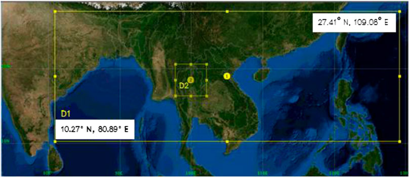
FIGURE 1. Domain configuration.
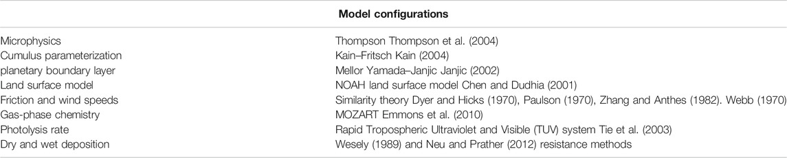
TABLE 1. Model configuration.
The model predictions of the O3, CO, and NO2 levels from WRF-Chem were compared to observations from the Pollution Control Department (PCD) in Thailand during March 2014. The PCD provides ground-based air quality observations in Thailand. The Thai PCD monitors six chemical species’ hourly surface concentrations: CO, O3, SO2, CO, PM2.5, NO2, and PM10. In Thailand, the measurement sites were urban, and, therefore, urban (especially motor vehicle) emissions dominated. The reference method or equivalent methods were used to measure the data. Almost every O3 observation was obtained using Model 400 (http:/www.teledyne-api.com/products/400e.asp) Teledyne Advant Policy Instrumentation. The detection limit of the instrument is lower by 0.6 ppbv and 1% accuracy. Nearly all of the CO observations were obtained using Teledyne Advanced Pollution Instrumentation Model 300, with a lower detection limit of 40 ppbv and a 0.5% detection precision (http:/www.teledyne-api.com/products/300e). There is regular missing information in PCD measurements, but only 15 percent of the time. In order to evaluate the model’s performance, a range of statistical methods was used, including the mean absolute error (MB) and the index of agreement (IOA).
where M = predicted concentration, O = observed concentration, and n = number of data.
The output of the model from the inner domain, that is, the precipitation and 2 m temperature, and O3, CO, and NO2 output, was compared to the ground-based measurement from the Thai PCD. Statistical analyses such as index of agreement (IOA), mean absolute error (MAE), and mean bias (MB) were utilized to examine the model performance (Table 2). The simulations of WRF-Chem were fairly consistent with the observations from PCD. The monthly mean 2 m temperature and precipitation from the model were agreeable, with IOAs in the range of 0.354–0.726 for temperature and 0.47 to 0.966 for precipitation, while the mean bias and MAE, respectively, were (−0.05)°C to 0.04°C and 0.6 to 1.5°C for temperature, and (−0.03) to 0.02 and 0.2mm–1.4 mm for precipitation. In general, the chemical species from the model were in fair agreement with those in observations, with IOA values in the range of 0.128–0.713. In comparison with the observations, however, the modeled chemical species were underestimated. In addition, WRF-Chem predicted levels of chemical species (CO and NO2) moderately well, with IOA values in the range of 0.445–0.713 for CO and 0.350–0.547 for NO2. The mean bias and MAE, respectively, were (−0.2) to 0.1 ppmv and 5.8 to 14.1 ppmv for O3; (−0.02) to 0.01 ppmv and 0.2 to 0.6 ppmv for CO; and (−0.4) to 0.04 ppmv and 2.6 to 12.9 ppmv for NO2. The discrepancies likely occur due to calculating all chemical species through the plum-rised model in WRF-Chem from aggregated coarse-resolution data of biomass-burning emissions, which was discussed in Amnuaylojaroen et al. (2014). These calculations capture a significant portion of the fire thermal buoyancy, which transports these species to high altitudes. A limitation is that the model configuration in this work did not consider the effect of aerosol feedback on the meteorology, which likely causes changes in temperature, boundary layer height, and clouds. These factors are likely to affect the results of O3 simulation (Forkel et al., 2012).
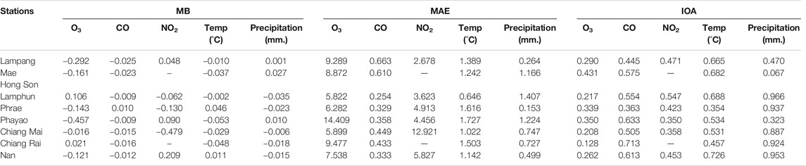
TABLE 2. Statistical analysis of ozone (O3), carbon monoxide (CO), nitrogen dioxide (NO2), temperature, and precipitation between the weather research and forecasting (WRF) model and ground-based measurements.
The output from domain two was used to illustrate the difference between WRF-CHEM simulations, including biomass burning emissions and WRF-CHEM simulations, excluding biomass burning emissions for monthly O3, CO, and NO2 concentrations in March 2014 (Figure 2). Biomass burning contributed between approximately 3–7% to background O3 (Figure 2A), where increases in the average monthly O3 concentration of approximately 3–4 ppmv were mostly observed in Northern Thailand (Figure 2D). Furthermore, biomass burning emissions substantially contributed to both CO and NO2 levels—approximately 60–90% (Figures 2B,C)—which increased the average monthly CO and NO2 concentrations by approximately 400 to 500 ppmv and 9 to 11 ppmv, respectively (Figures 2E,F). The majority of significant biomass burning—contributing to more than 90% of surface NO2—occurred in Northern Thailand (Figure 2F).
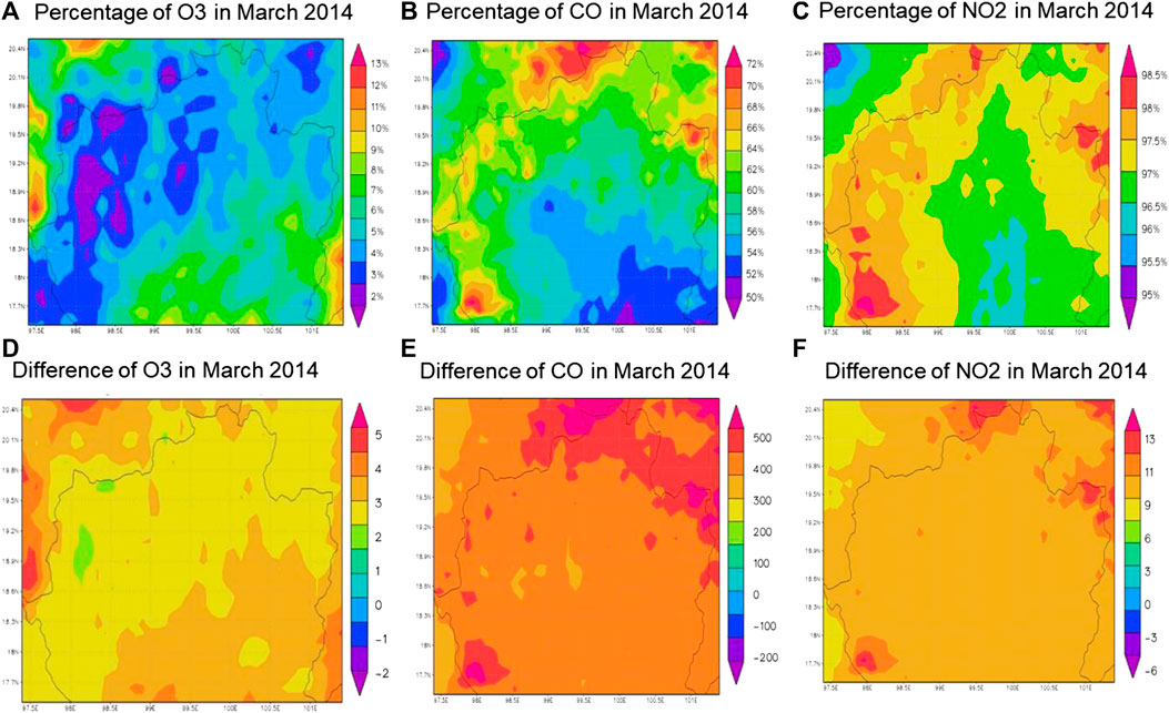
FIGURE 2. Percentage (upper panel) and absolute (bottom panel) differences in O3(A and D), CO (B and E), and NO2(C and F) concentrations between the two WRF-Chem simulations with and without biomass burning emissions.
According to the model simulation, biomass burning emissions have a small effect on the increase in O3 concentration, but a significant one on the increase in CO and NO2 concentrations in Northern Thailand. These results are similar to those of the previous study; for example, Galanter et al., 2000 found that biomass burning is a major source of NOx and CO in the tropical region, which contributes >50% of atmospheric CO and NOx. In addition, Granier et al., 2000 argued that biomass burning emissions make a significant contribution to the tropospheric O3 budget, particularly in the tropical region. Because biomass burning emissions directly add to NO2 and CO levels, the resulting impact on O3 is buffered by the nonlinear response of ozone chemistry and transport (Galanter al., 2000); processes controlling surface O3 production are likely due to another factor in its chemistry. As discussed in the study by Amnuaylojaroen et al., 2019, the net O3 production in upper Southeast Asia is NOx-limited, which is insensitive to both constant NOx and VOC decreases—the production of BIGENE (note that BIGENE represents lumped alkenes, Emmons et al., 2010) and CO peroxy radicals mainly dominates the reaction rate for O3 production. In addition, biomass burning emissions slightly increase the BIGENE and CO reaction rates. However, this research does not consider the impact of the transport of biomass burning plumes that also play an important role in increasing the O3 mixing ratios. As discussed by Kondo et al., 2004, the increase in the mixing ratios of O3 and its precursors in the western Pacific due to biomass burning in Southeast Asia was estimated using the tracers. Additionally, Brocchi et al., 2018 found that the intercontinental transport of biomass burning from Siberia and Canada qualitatively reproduced CO and O3 concentration variations in the Mediterranean Basin.
During the peak period of biomass burning, we applied a regional model of atmospheric chemistry to study the effect of biomass burning on O3, CO, and NO2 concentrations in Northern Thailand. The model can be used to analyze, with acceptable precision, the contributions of biomass burning to surface O3, CO, and NO2 levels. By comparing the model results with ground-based measurements in Thailand, we found that the model was generally consistent with precipitation, the temperature at 2 m, and O3, CO, and NOx levels. However, in most areas of Northern Thailand, the model generally underestimated the magnitude of all chemical species. A comparison of WRF-CHEM simulations with and without burning biomass emissions showed an increase in O3, CO, and NOx levels due to biomass burning. Biomass combustion, however, contributed directly to over 60% of CO and NO2 levels and indirectly to the concentration of O3 in Northern Thailand. Compared to CO and O3, biomass burning had the greatest impact on the NO2 distribution, contributing to over 90% of total NO2 background levels, while biomass burning slightly contributed to surface O3 levels, by approximately 7%.
The original contributions presented in the study are included in the article/Supplementary Material; further inquiries can be directed to the corresponding author.
TA: conceived and designed the experiments; performed the experiments; analyzed and interpreted the data; contributed reagents, materials, analysis tools, or data; and wrote the article. SK: contributed reagents, materials, analysis tools, or data.
This research was funded by the University of Phayao, Thailand. FF64-UoE015.
The authors declare that the research was conducted in the absence of any commercial or financial relationships that could be construed as a potential conflict of interest.
We also acknowledge the use of the WRF-Chem preprocessor tool {mozbc, fire_emiss, bio_emiss, anthro_emiss} provided by the Atmospheric Chemistry Observations and Modeling (ACOM) lab of the NCAR. Finally, we also acknowledge the Pollution Control Department for providing the ground-based measurement data in northern Thailand.
Amnuaylojaroen, T., Barth, M. C., Emmons, L. K., Carmichael, G. R., Kreasuwun, J., Prasitwattanaseree, S., et al. (2014). Effect of different emission inventories on modeled ozone and carbon monoxide in Southeast Asia. Atmos. Chem. Phys. 14, 12983–13012. doi:10.5194/acp-14-12983-2014
Amnuaylojaroen, T., Barth, M. C., Pfister, G. G., and Bruyere, C. C. (2018). “Simulation of emissions, air quality, and climate contribution in Southeast Asia for March and december,” in Land-atmospheric research applications in South and Southeast Asia, springer remote sensing/photogrammetry. Editors K. Vadrevu, T. Ohara, and C. Justice (Cham, Switzerland: Springer), 233–254. doi:10.1007/978-3-319-67474-2_12
Amnuaylojaroen, T., Inkom, J., Janta, R., and Surapipith, V. (2020). Long range transport of Southeast asian PM2.5 pollution to northern Thailand during high biomass burning episodes. Sustainability 12 (23), 10049. doi:10.3390/su122310049
Amnuaylojaroen, T., Macatangay, R. C., and Khodmanee, S. (2019). Modeling the effect of VOCs from biomass burning emissions on ozone pollution in upper Southeast Asia. Heliyon 5 (10), e02611. doi:10.1016/j.heliyon.2019.e02661
Brocchi, V., Krysztofiak, G., Catoire, V., Guth, J., Marécal, V., Zbinden, R., et al. (2018). Intercontinental transport of biomass burning pollutants over the Mediterranean Basin during the summer 2014 ChArMEx-GLAM airborne campaign. Atmos. Chem. Phys. 18, 6887–6906. doi:10.5194/acp-18-6887-2018
Chang, D., and Song, Y. (2010). Estimates of biomass burning emissions in tropical Asia based on satellite-derived data. Atmos. Chem. Phys. 10, 2335–2351. doi:10.5194/acp-10-2335-2010
Chen, F., and Dudhia, J. (2001). Coupling an advanced land surface-hydrology model with the penn state-NCAR MM5 modeling system. Part I: model implementation and sensitivity. Mon. Wea. Rev. 129, 569–585. doi:10.1175/1520-0493(2001)129<0569:caalsh>2.0.co;2
Dyer, A. J., and Hicks, B. B. (1970). Flux-gradient relationships in the constant flux layer. Q J R. Met. Soc. 96, 715–721. doi:10.1002/qj.49709641012
Emmons, L. K., Walters, S., Hess, P. G., Lamarque, J.-F., Pfister, G. G., Fillmore, D., et al. (2010). Description and evaluation of the model for ozone and related chemical tracers, version 4 (MOZART-4). Geosci. Model. Dev. 3, 43–67. doi:10.5194/gmd-3-43-2010
Forkel, R., Werhahn, J., Hansen, A. B., Mckeen, S., Peckham, S., Grell, G., et al. (2012). Effect of aerosol-radiation feedback on regional air quality—a case study with WRF/Chem. Atmos. Environ. 53, 202–211. doi:10.1016/j.atmosenv.2011.10.009
Galanter, M., Levy, H., and Carmichael, G. R. (2000). Impacts of biomass burning on tropospheric CO, NOx, and O3. J. Geophys. Res. 105 (D5), 6633–6653. doi:10.1029/1999jd901113
Granier, C., Müller, J. F., and Brasseur, G. (2000). “The impact of biomass burning on the global budget of ozone and ozone precursors,” in Biomass burning and its inter-relationships with the climate system. Dordrecht, Netherlands: Springer, 69–85.
Grell, G. A., Peckham, S. E., Schmitz, R., McKeen, S. A., Frost, G., Skamarock, W. C., et al. (2005). Fully coupled “online” chemistry within the WRF model. Atmos. Environ. 39, 6957–6975. doi:10.1016/j.atmosenv.2005.04.027
Guenther, A., Karl, T., Harley, P., Wiedinmyer, C., Palmer, P. I., and Geron, C. (2006). Estimates of global terrestrial isoprene emissions using MEGAN (model of emissions of Gases and aerosols from nature). Atmos. Chem. Phys. 6, 3181–3210. doi:10.5194/acp-6-3181-2006
Janjic, Z. I. (2002). Nonsingular implementation of the mellor–yamada level 2.5 scheme in the NCEP meso model, national oceanic and atmospheric administration science center, camp springs, MD. NCEP Off. Note, No. 437, 61.
Janssens-Maenhout, G., Crippa, M., Guizzardi, D., Dentener, F., Muntean, M., Pouliot, G., et al. (2015). HTAP_v2.2: a mosaic of regional and global emission grid maps for 2008 and 2010 to study hemispheric transport of air pollution. Atmos. Chem. Phys. 15, 11411–11432. doi:10.5194/acp-15-11411-2015
Kain, J. S. (2004). The Kain-Fritsch convective parameterization: an update. J. Appl. Meteorol. 43, 170–181. doi:10.1175/1520-0450(2004)043<0170:tkcpau>2.0.co;2
Kondo, Y. (2004). Impacts of biomass burning in Southeast Asia on ozone and reactive nitrogen over the western Pacific in spring. J. Geophys. Res. 109. doi:10.1029/2003jd004203
Neu, J. L., and Prather, M. J. (2012). Toward a more physical representation of precipitation scavenging in global chemistry models: cloud overlap and ice physics and their impact on tropospheric ozone. Atmos. Chem. Phys. 12, 3289–3310. doi:10.5194/acp-12-3289-2012
Parrington, M., Palmer, P. I., Henze, D. K., Tarasick, D. W., Hyer, E. J., Owen, R. C., et al. (2012). The influence of boreal biomass burning emissions on the distribution of tropospheric ozone over North America and the North Atlantic during 2010. Atmos. Chem. Phys. 12 (4), 2077–2098. doi:10.5194/acp-12-2077-2012
Paulson, C. A. (1970). The mathematical representation of wind speed and temperature profiles in the unstable atmospheric surface layer. J. Appl. Meteorol. 9, 857–861. doi:10.1175/1520-0450(1970)009<0857:tmrows>2.0.co;2
Pfister, G. G., Emmons, L. K., Hess, P. G., Honrath, R., Lamarque, J.-F., Val Martin, M., et al. (2006). Ozone production from the 2004 North American boreal fires. J. Geophys. Res. 111, D24S07. doi:10.1029/2006JD007695
Seinfeld, H. J., and Pandis, S. N. (1998). Atmospheric chemistry and physics from air pollution to climate change. Hoboken, NJ: John Wiley and Sons.
Sharma, A., Ojha, N., Pozzer, A., Mar, K. A., Beig, G., Lelieveld, J., et al. (2017). WRF-Chem simulated surface ozone over south Asia during the pre-monsoon: effects of emission inventories and chemical mechanisms. Atmos. Chem. Phys. 17 (23), 14393–14413. doi:10.5194/acp-17-14393-2017
Sonkaew, T., and Macatangay, R. (2015). Determining relationships and mechanisms between tropospheric ozone column concentrations and tropical biomass burning in Thailand and its surrounding regions. Environ. Res. Lett. 10 (6), 065009. doi:10.1088/1748-9326/10/6/065009
Thompson, G., Rasmussen, R. M., and Manning, K. (2004). Explicit forecasts of winter precipitation using an improved bulk microphysics scheme. Part I: description and sensitivity analysis. Mon. Wea. Rev. 132, 519–542. doi:10.1175/1520-0493(2004)132<0519:efowpu>2.0.co;2
Tie, X., Madronich, S., Walters, S., Zhang, R., Rasch, P., and Collins, W. (2003). Effect of clouds on photolysis and oxidants in the troposphere. J. Geophys. Res. 108, 4642. doi:10.1029/2003JD003659
Webb, E. K. (1970). Profile relationships: the log-linear range, and extension to strong stability. Q J R. Met. Soc. 96, 67–90. doi:10.1002/qj.49709640708
Wesely, M. L. (1989). Parameterization of surface resistances to gaseous dry deposition in regional-scale numerical models. Atmos. Environ. 23, 1293–1304. doi:10.1016/0004-6981(89)90153-4
Wiedinmyer, C., Akagi, S. K., Yokelson, R. J., Emmons, L. K., Al-Saadi, J. A., Orlando, J. J., et al. (2011). The Fire Inventory from NCAR (FINN): a high resolution global model to estimate the emissions from open burning. Geosci. Model. Dev. 4, 625–641. doi:10.5194/gmd-4-625-2011
Xing, L., Li, G., and Han, Y. (2019). The impact of biomass burning in peninsular Southeast Asia on PM2.5 and ozone formation over southern China in spring. AGUFM. 2019, A31K–A2847.
Keywords: biomass burning, ozone, carbon monoxide, nitrogen dioxide, Southeast Asia
Citation: Khodmanee S and Amnuaylojaroen T (2021) Impact of Biomass Burning on Ozone, Carbon Monoxide, and Nitrogen Dioxide in Northern Thailand. Front. Environ. Sci. 9:641877. doi: 10.3389/fenvs.2021.641877
Received: 15 December 2020; Accepted: 21 January 2021;
Published: 08 April 2021.
Edited by:
Manousos-Ioannis Manousakas, Paul Scherrer Institut (PSI), SwitzerlandReviewed by:
Mohd Talib Latif, National University of Malaysia, MalaysiaCopyright © 2021 Khodmanee and Amnuaylojaroen. This is an open-access article distributed under the terms of the Creative Commons Attribution License (CC BY). The use, distribution or reproduction in other forums is permitted, provided the original author(s) and the copyright owner(s) are credited and that the original publication in this journal is cited, in accordance with accepted academic practice. No use, distribution or reproduction is permitted which does not comply with these terms.
*Correspondence: Teerachai Amnuaylojaroen, dGVlcmFjaGFpNEBnbWFpbC5jb20=
Disclaimer: All claims expressed in this article are solely those of the authors and do not necessarily represent those of their affiliated organizations, or those of the publisher, the editors and the reviewers. Any product that may be evaluated in this article or claim that may be made by its manufacturer is not guaranteed or endorsed by the publisher.
Research integrity at Frontiers
Learn more about the work of our research integrity team to safeguard the quality of each article we publish.