Determining Building Natural Ventilation Potential via IoT-Based Air Quality Sensors

Natural ventilation (NV) represents the most energy-efficient way to operate buildings and, in an attempt to reduce the built environment's global carbon footprint, represents a resource, the usage of which has to be maximized. This study demonstrated how a combination of an IoT environmental sensing network implemented locally outdoors and indoors can help to determine the NV potential and actual utilization throughout the year with the consideration of outdoor climate variance, air pollution levels, and window open/closed status. An NV potential index was developed by analyzing indoor and outdoor PM_2.5, and outdoor air temperature and air speed throughout the year at different spatial (from room scale to building level and local weather stations) and temporal (instantaneous, season, and annual) scales. The index was applied on a case building located in Berkeley, California, during the period of August 2018 to the end of 2019. Compared to the potential NV availability, the actual window opening time in typical rooms was less than 35%. These results point out that the actual window usage behavior was the key limiting factor in NV potential utilization. Even during periods when climate- and pollution-wise outdoor conditions allowed use of the NV, many occupants kept their windows closed. Keeping windows open or closed was significantly affected by outdoor climate condition and air pollution levels, especially during the wild-fire period.

Introduction

People spend nearly 90% of their daily lives indoors and rely on mechanical heating, ventilation, and air-conditioning (HVAC) systems to maintain indoor environments comfortable. The building sector accounts for 40% of total energy use and around one-third of CO₂ emission in major economies such as Europe (Commission, 2010), the United States (EIA, 2021), and China (Xiong et al., 2015). A large proportion of this energy was consumed by HVAC systems, which is particularly true in cold and tropical climate zones where the outdoor climate intensifies the HVAC usage. In response to the high energy consumption of mechanical HVAC systems, there has been an increase in research on natural ventilation (NV), and alternative indoor environment conditioning strategies for residential (Oropeza-Perez and Østergaard, 2014) and commercial buildings (da Graça et al., 2004).

Natural Ventilation

NV refers to the process of supplying air to and removing air from an indoor space without using mechanical systems. Taking advantage of pressure differences arising from natural forces, for example, wind-driven force and buoyancy-driven force, the external air flows into an indoor space, while the internal air flows out (Asfour, 2015). With a proper design, NV can replace cooling systems in the milder months of the year, reducing ventilation- and cooling-related energy demand (Dutton et al., 2013). The NV strategy can also be integrated with the mechanical HVAC system, forming a mixed-mode strategy that allows alternatives between the HVAC and NV throughout the day or the year depending on weather conditions (Luo et al., 2015). The advantages of applying the NV strategy in buildings include but are not limited to 1) reducing operation costs, 2) increasing occupants’ thermal comfort, and 3) improving air quality due to more fresh air.

While many studies emphasize the advantages of NV, the actual NV use can be affected by many external factors such as the outdoor climate and pollutant levels (Zhou et al., 2015; Costanzo et al., 2019). The results of the study by Martins and Carrilho da Graça (2017) showed that using NV in moments when the outside weather is favorable can result in HVAC energy savings of 25–80%. However, limiting NV use to moments with outdoor particle levels below 12 μg/m³ decreases this energy-saving potential to 20–60%. In the majority of the cities analyzed in the study by Martins and Carrilho da Graça (2017), the use of NV led to an increase in indoor exposure to PM_2.5 of outdoor origin of 400–500%. Additionally, building occupants’ habits and altitudes in interacting with building openings like the windows will also affect the NV performance by a large margin. Therefore, understanding how these factors would limit the NV usage and how to consider these factors in real-building NV operation are of great value.

On the one hand, many studies have investigated the correlations between window status and the outdoor climate conditions. Raja et al. (Raja et al., 2001) studied the relationship of windows, doors, blinds, fans, etc. with indoor and outdoor temperatures in 15 naturally ventilated office buildings in Oxford and Aberdeen, in the UK, during a summer period. It is found that proportion of open windows increases with an increase in indoor and outdoor temperature. Only few windows are open when the outdoor temperature is below 15°C, whereas most windows are open when the temperature exceeds about 25°C. Nicol and Humphrey (2001) surveyed the window usage in naturally ventilated buildings in the UK, Sweden, France, Portugal, Greece, and Pakistan. They found that occupants started to open windows at a temperature above 10°C, and as the temperature rises, there is an increased probability that a window will be open. Based on the observations in the literature, the percentage of open windows, opening hours, and the frequency of opening or closing windows depend on seasons, outdoor temperature, indoor temperature, time of the day, and the presence of the occupants. For a well-designed building with low internal gains, user-controlled windows may be opened for outdoor temperatures for as low as 10°C (Raja et al., 2001). The typical maximum outdoor temperature for NV use in an office is 28°C (de Dear and Brager, 2002); above this temperature, the indoor environment tends to become uncomfortably warm.

On the other hand, few studies have considered outdoor particle levels as limiting factors of NV use. When the building operates in the NV mode, windows will be opened to promote the large outdoor airflows that are required for ventilated cooling so that indoor exposure to outdoor particulate matter (PM) can be significant, with I/O ratios that are close to one (Martins and Carrilho da Graça, 2017). To avoid this problem, a building connected to an outdoor PM_2.5 sensor network must close the NV openings and revert to conventional HVAC during periods of high PM_2.5. This requirement reduces the number of hours when NV can be used and requires HVAC energy consumption during these periods. It is likely that the magnitude of this impact will depend on the local weather condition and particle source patterns, as particles suspended in the outdoor air are in an unstable state and their concentration can be changed by meteorological conditions, such as precipitation and wind sweeping. In the majority of urban environments, outdoor air is a source of pollutants that have a detrimental impact on indoor air quality (IAQ). There is strong evidence of adverse health effects from exposure to airborne particles that are small enough to be inhaled (diameter below 10 µm (Fenger, 2009; Talbott et al., 2015)). Limiting airborne particle exposure has long been a priority of the World Health Organization (WHO), leading to continuously updated guidelines for maximum short-term and annual mean exposures to airborne particles (WHO Regional Office for Europe, 2013). Continued exposure to PM_2.5 in amounts that are just above the natural background concentration of 3–5 μg/m³ can cause adverse health effects (Nicol and Humphrey, 2001). The combination of a mostly anthropogenic origin and an increased exposure risk makes PM_2.5 the preferred indicator for assessing health impacts from outdoor particles.

The Emergence of IoT Sensing Technology

Internet of Things (IoT) environmental sensing platforms for the measurement of various environmental parameters are deployed on the urban and building scale. Low-cost sensing platforms provide higher measurement granularity than the government-owned and operated air quality station on an urban scale (Morawska et al., 2018). On a building scale, a number of different environmental sensing platforms are deployed to enable visibility of indoor conditions to building managers and potentially occupants (Parkinson et al., 2019). These two fields of science and engineering are currently kept entirely separate, with a single publication showing the potential of integrating indoor and outdoor data for effective building operations during wildfire (Pantelic et al., 2019). There is a clear gap in understanding of how to use available information to better operate buildings or to understand key aspects of how buildings work, especially naturally ventilated buildings that are dependent on outdoor conditions, indoor conditions, and the behavior of occupants.

Objectives of This Study

This study aimed to demonstrate how a combination of an IoT environmental sensing network implemented locally outdoors and indoors can help to determine NV potential and actual utilization in the building throughout the year. NV potential is evaluated by considering outdoor climate variance and air pollution levels, and the actual NV use was evaluated using environmental data and occupant behavior with respect to the use of windows. In doing this, we analyzed indoor and outdoor PM_2.5, indoor CO₂, and outdoor air temperature throughout the year at different spatial (from room scale to building level and local weather stations) and temporal scales (instantaneous and long-term) to demonstrate the application of NV assessment tools. We used an NV case building located in Berkeley (California) during the period of August 2018 to the end of 2019. By reliance on an NV potential index considering outdoor PM_2.5, temperature, and wind speed, the study sought to quantify the NV availability throughout the year.

Materials and Methods

Experimental Design

The IoT sensing network was deployed in Wurster Hall, a 9-floor mixed-mode operated building in Berkeley, CA. During the spring, summer, and autumn, the building is operated in the natural ventilation mode, while in winter there is mechanical heating. When the building operates in the NV mode, it relies on operable windows for ventilation and cooling. The building has a high level of infiltration, as shown by typical CO₂ levels below 550 ppm during normal operation. The building has multiple function rooms, such as a classroom, conference room, private, and open offices, with approximately 300 full-time occupants.

The IoT sensing network was deployed on July 19, 2018, and the study ended in December 2019. During this time period, the town of Berkeley was affected by the Chico Camp wildfire from November 18, 2018 to November 25, 2018. This offered a great opportunity to investigate how high outdoor particulate pollutants would affect the NV use and how building occupants would respond to these episodes. When doing the test, the building level of outdoor temperature and PM_2.5 concentration, room level of indoor CO₂ and PM_2.5 concentrations, and window status were monitored. The indoor sensors were installed in 15 rooms (the room number and room functions are listed in Table 1), including classrooms, meeting rooms, and office rooms. Figure 1 shows the locations of installed sensors on the third floor. The window closure sensors were installed at the bottom or on the side of the frame of openable windows. The CO₂ and PM_2.5 sensors were installed on the walls ∼1.2 m from the floor.

TABLE 1

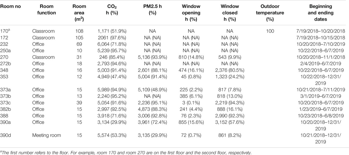
TABLE 1. Available data amount for different variables.

FIGURE 1

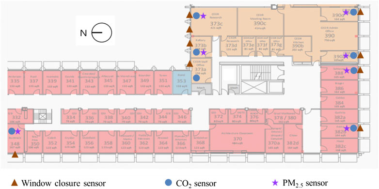
FIGURE 1. The locations of the indoor sensors installed on the third floor. There are other indoor sensors on the first and the second floors (see Table 1 for more information). The 9-floor case building is located in Berkeley, California, the United States.

The study also contained surveys of building occupants about their motivations or reasons for open windows. Detailed survey questions can be found in the Appendix. Questions could be classified into several categories of which there are three main aspects related to thermal comfort, air quality, and psychological motivations.

Experimental Apparatus

The study utilized two types of indoor PM_2.5 sensors (Clarity Inc., and Senseware) and outdoor PM_2.5 sensor (Clarity Inc.). The outdoor sensors were installed at the top of Wurster Hall, a 9-floor building. Indoor sensors were placed in different spaces in Wurster Hall (see Figure 1 as examples). Both Clarity and Senseware PM_2.5 nodes count the particle number using the principle of light scattering. The accuracy of all the sensors was the same—within ± 10 μg/m³ in the range of 0–100 μg/m³ and ±10% in the range of 100–1,000 μg/m³. Data were collected at 15 min intervals for Clarity nodes and 1 min intervals for Senseware nodes. Clarity and Senseware PM_2.5 nodes are factory-calibrated with Arizona Test Dust (ATD). To accurately measure PM_2.5 concentrations, the Clarity nodes apply colocation of nodes and post-processing correction factors based on referencing government air quality stations. We colocated all sensors and adjusted readings. Indoor CO₂ levels were measured by Senseware CO₂ sensors with an accuracy of ±50 ppm from 400 ppm to 2000 ppm. The CO₂ sensors were paired with PM_2.5 measurements.

Window status was monitored with Senseware contact sensors (Model COZIR-LP) placed on the windows. The detection was binary (i.e., open/closed) and did not provide information on the opening area or window angle. The on/off signals from the sensors enable us to know generally if the window was open or closed, but not to which extent the window was open. All the windows in the buildings were awning type, opening outward for up to 45°. Friction hinges on the windows were able to maintain the angle after they were open. The contact sensors sensed status information through Senseware IoT platform every 5 min.

Weather conditions including outdoor temperature and wind speed were collected from the Weather Underground webpage from the Oakland-9925 International Boulevard, which is 16 km from Wurster Hall. Outdoor PM_2.5 concentrations were collected from California Air Quality Board webpage from the Oakland-9925 International Boulevard (station 1), Berkeley Aquatic Part (station 2), and Oakland-Laney College stations (station 3), which are 10, 16, and 9 km away from Wurster Hall, respectively. PM_2.5 and CO₂ concentrations were also measured at the edge of the roof of Wurster Hall.

Data Analysis

Missing Data and Quality Control

All the data collected were averaged by hour, and then, the number of hours in each room was counted. The sum of the total hours for each room equals the length of effective time of each room. Therefore, the interval between recording data can be ignored (data are recorded in different intervals by two nodes of sensors). The starting and ending dates of each room are different, and in some rooms, data were recorded only partially. This means that the period with valid data is often less than the whole monitoring period. The total duration of the data is 12,744 h. The median percentage of valid data for CO₂, PM_2.5, and window closure is 31, 35, and 69%, respectively. The amount of data recorded when the window is closed is significantly higher than that of data recorded when the window is open, and their medians are 55.6 and 12.9%, respectively. Data on outdoor temperature are available throughout the study period.

The percentage of valid data varied between rooms. For example, the room with the largest amount of valid data of CO₂ is room 172, while the room with the smallest amount of CO₂ is room 390a. The percentage of valid data of PM_2.5 in each room is similar to that of valid data of CO₂. For room 170, room 172, room 232, and room 373a, the PM_2.5 and window closure data were not recorded. With these data, we developed and evaluated tools to quantify and assess the building’s NV potential throughout the year.

Evaluation Method

Indoor PM_2.5concentration threshold. The World Health Organization (WHO) guidelines for PM_2.5 of 25 μg/m³ for 24 h mean exposure were chosen to evaluate building operation. WHO guidelines have the strictest concentration limit and the best health outcome for the exposed occupants. Alternative guidelines such as those of the Environmental Protection Agency (EPA) may be used in other local regions of the world. When doing the comparison, the median hourly indoor PM_2.5 concentration (i.e., median value from all indoor sensors) was compared to WHO 24 h mean exposure guideline using the Exceedance index (E-index), as shown in Eq. 1. The E-index is a unitless value that is informed by how much hourly PM_2.5 concentration exceeds the recommended level. Using this index, percentage of hours that indoor PM_2.5 concentration exceeds specified levels during the air pollution episode can be calculated so that it can evaluate occupant exposure to extreme air pollution events across buildings or on a space-by-space basis within the same building.

$E=\frac{C_{measuredP{M}_{2.5}}}{25\mu g/m^3}.(1)$

In addition to indoor PM_2.5 exposure evaluation, it is also important to know how outdoor pollution levels would affect indoor pollutions. The I/O ratios, shown in Eq. 2, were applied to quantify building resilience to penetration and infiltration of outdoor PM_2.5.

$I/O=\frac{C_{in}\left(t\right)}{C_{out}\left(t\right)}.(2)$

The I/O ratio was calculated for each indoor sensor location using hourly mean indoor and outdoor PM_2.5 concentration (Eq 2, where C_in(t) and C_out(t) are the hourly means). To calculate the whole building instantaneous I/O ratio, the median hourly mean PM_2.5 from the indoor sensors was compared to the hourly mean outdoor PM_2.5 concentrations. The median values were used instead of the mean values because they were robust to outlier instances.

Indoor CO₂ levels were compared with the 700 ppm thresholds for sedentary activities plus the typical outdoor value that is 400 ppm for Berkeley, CA.

When doing the analysis, working hours were from 8:00 am to 18:00 pm, while other hours were nonworking hours. Weekdays include Monday, Tuesday, Wednesday, Thursday, and Friday, while Saturday and Sunday were weekends. The time periods from 2018-8-15 to 2018-8-28 and from 2018-11-08 to 2018-11-25 were marked as “wildfire,” and other periods were noted as “non-wildfire.”

NV Potential Index

The NV potential was defined as a measure to check if the outdoor weather and air quality condition were favorable for NV. It can be derived from outdoor meteorological data and air pollution level. Detailed methodologies regarding NV availability calculation can be seen in previous studies (Yin et al., 2010; Chen et al., 2017).

Regarding the outdoor temperature, two common methods were employed to determine whether it is favorable for NV. The first approach is to set fixed upper and lower limits throughout the year. As shown in Eq. 3, 12.8°C and 26°C were set as the lower limit and the upper limit, respectively, which means that NV is assumed to be available when outdoor temperature is between 12.8°C and 26°C (Herkel et al., 2008; ASHRAE Standard 55-2013 Thermal Environmental Conditions for Human Occupancy (ANSI Approved), 2013). Another approach is to take advantage of the adaptive comfort model proposed by de Dear and Brager (de Dear and Brager, 2002), which allows the upper limit (T_up) to vary by month. Eq. 4 shows the calculation of the upper temperature limit, where T_out is the monthly average outdoor temperature determined from weather data. $\Delta {\text{T}}_{80\text{\%}}$ is the 80% acceptability comfort zone band, which is equal to 7°C, while the 90% acceptability comfort zone band should be 5°C. Favorable temperature thresholds are when the outdoor temperature is below the upper limit (T_up) but greater than lower limit (T_low) of 12.8°C.

$12.8\mathit{°}C\le T_{out}\le 26\mathit{°}C,(3)$

$T_{up}=0.31T_{out}+17.8+\frac{1}{2}\Delta T_{80\%}.(4)$

The maximum outdoor wind speed ($u_{out,max}$) was derived by Eq. 5 that was developed by Phaff et al. (1980), whereas the maximum allowable indoor air velocity $u_{in,max}$ is 0.8 m/s (ASHRAE Standard 55-2013 Thermal Environmental Conditions for Human Occupancy (ANSI Approved), 2013). $\Delta T_{max}$ is the hourly maximum temperature difference between the outdoor temperature and indoor temperature during NV hours. Here, $\Delta T_{max}$ was approximated as the difference between the upper temperature limit (T_up) and the lower temperature limit (T_low). C1 is the wind speed coefficient, C2 is the buoyancy coefficient, and C3 is the turbulence coefficient. Their values are C₁ = 0.001, C₂ = 0.0035 (ms⁻² K⁻¹), and C₃ = 0.01 (m²·s⁻²) (Phaff et al., 1980).

$u_{in,max}=\sqrt{C_1{u}_{out,\max }^2+C_{2}h\Delta T_{\max }+C_3}.(5)$

As for the outdoor particle pollution level, PM_2.5 concentration was selected to reflect the outdoor air quality. It is assumed that when the outdoor PM_2.5 is below or equal to 25 μg/m³, that is, the limit set by both the WHO and EPA, the outdoor air quality is favorable for NV.

Statistical Tools Used

The IoT sensing and occupant survey data were analyzed using R version 3.6.1 software (The R Foundation, 2021). Statistical analysis was performed on the measured sensor data to compare between sensor locations (i.e., among different rooms and different regional weather stations) and to compare survey responses between typical pollutant conditions (i.e., wildfire and non-wildfire periods). The data under consideration were not normally distributed, so the nonparametric tests were adopted. To assess statistical significance between the measured PM_2.5 concentrations or outdoor temperatures at different locations, a two-sided Wilcoxon rank-sum test, also known as the Mann–Whitney test, was used.

Results

Indoor/Outdoor PM_2.5, CO₂, and Temperature

Figure 2 shows the overall distribution of hourly average indoor and outdoor PM_2.5, indoor CO₂, and outdoor temperature during the period from July 19, 2018 to the end of 2019. During this period, the median outdoor PM_2.5 concentration was 3.5°μg/m³, slightly higher than the 1.4 μg/m³ of indoor PM_2.5. A majority of the PM_2.5 concentration values, 97.3% for outdoor and 95.5% for indoor, were lower than the recommended value of 25 μg/m³. With a median value of 437.2°ppm, the measured indoor CO₂ concentration was low, 94.0% of the time was lower than 500°ppm and 72.3% of the time was lower than 450°ppm. The outdoor temperature ranged from 11.5°C (lower quartile) to 17.4°C (upper quartile), with a median value of 14.0°C. But there were also few extreme weather conditions with outdoor temperatures lower than 10°C or higher than 30°C.

FIGURE 2

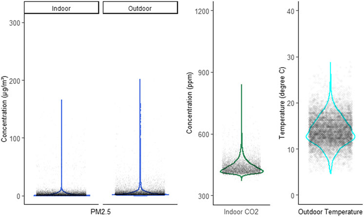
FIGURE 2. Hourly averaged indoor and outdoor PM_2.5, CO₂, and temperature.

To see how these parameters varied with time, Figure 3 presents them in the time series view. Most of the time, both indoor and outdoor PM_2.5 maintained at a level lower than 25 μg/m³. But there were some short periods, for example, August 15 to August 28 and November 8 to November 25 in 2018, and the PM_2.5 concentrations climbed up to as high as over 200 μg/m³. This sudden change in the pollutant level was caused by wildfire, which will be discussed in the later analysis. Different from the PM_2.5, the CO₂ concentration fluctuated over the study period, while the temperature was mainly affected by the season.

FIGURE 3

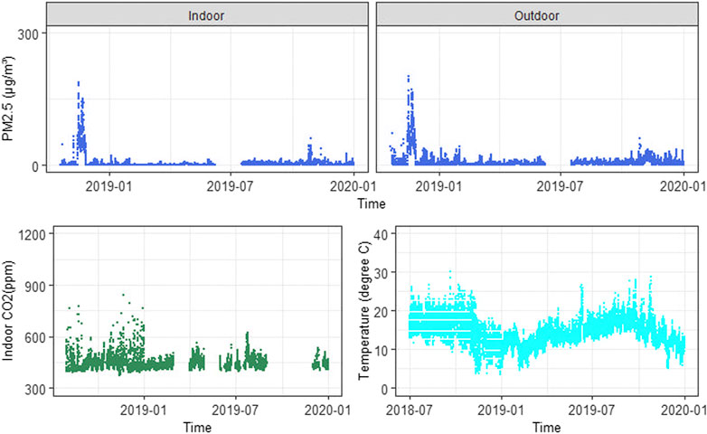
FIGURE 3. Time variance of indoor and outdoor PM_2.5, CO₂, and temperature.

Figure 4 shows the E index and I/O ratio of the PM_2.5 and CO₂ concentrations, respectively, for each room. When there was no wildfire, the indoor PM_2.5 concentrations were usually lower than 25 μg/m³ so that the E indexes were smaller than 1, and only 1.9% of E indexes were larger than 1. When there was a wildfire, the indoor PM_2.5 increased significantly, resulting in higher E indexes, and 93% of those are larger than 1. The observation can be validated by the I/O ratio which compares the indoor and outdoor PM_2.5 concentrations. For non-wildfire periods, the room level I/O ratios were usually below 0.5, with only 0.6% of spikes higher than 0.5. During the wildfire period, the I/O ratios climbed to 0.5–1 range. Different from PM_2.5, the indoor CO₂ concentration in different rooms was not significantly affected by extreme events like the wildfire.

FIGURE 4

FIGURE 4. Evaluation of indoor PM_2.5 and CO₂ concentration in different rooms.

Use of Windows

To investigate how the building occupants interacted with the windows, Figure 5 shows the use of windows at three levels. First, the building-level chart compares the night-time and working-time window usage during the wildfire period and that in the non-fire period. 21% of windows were open during the non-fire period, while all of the windows were closed if there was a wildfire. The window usage were similar in nighttime and working time. 24.3% windows were open during working hours, close to the 21.5% of night hours. Second, different room functions may have different window usage rates. The classroom with 63.1% of window open time used the windows more frequently than the meeting room and office room. Third, the window usages for each room varied significantly during the non-wildfire period. Some rooms opened the windows for over 50% of the time, while some others kept the window closed all the time. This observation suggests that usage pattern of the windows depends on the occupants’ behavior and also on the number of occupants in the room. Some occupants opened and closed the window actively, some did not.

FIGURE 5

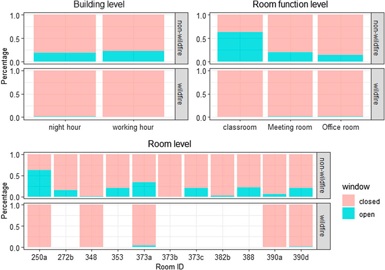
FIGURE 5. Window usage at different levels.

Figure 6 shows window usage during different outdoor conditions. The visible outdoor pollutants like the PM_2.5 significantly affect the window usage. Occupants tended to close windows when the outdoor pollutant level was “heavy” (PM_2.5 > 100 μg/m³) and open windows more when the outdoor pollutant level was “low” (PM_2.5 < 25 μg/m³). At the same time, the outdoor temperature can also affect the window usage. As the outdoor temperature increased from “cold” (<10°C) to “hot” (>26°C), there was an increasing percentage of opening windows.

FIGURE 6

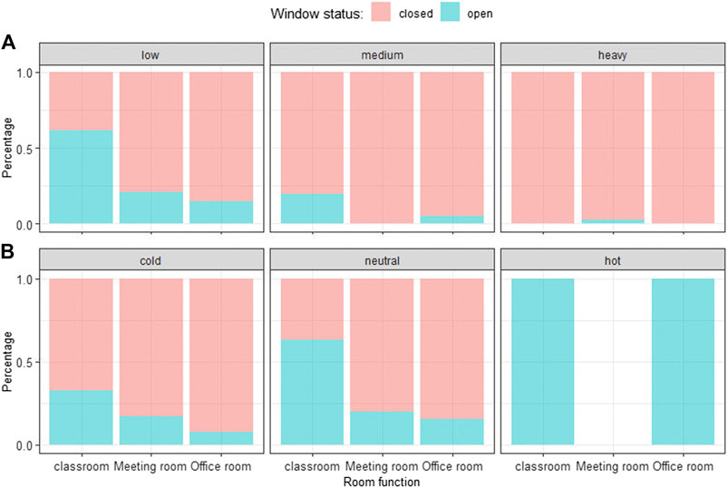
FIGURE 6. Window usage at different a) outdoor PM levels and b) outdoor air temperatures. The “low,” “medium,” and “heavy” PM2.5 levels are <25 μg/m³, 25–100 μg/m³, and >100 μg/m³, respectively. The “cold,” “neutral,” and “hot” outdoor air temperatures are <10°C, 10–26°C, and >26°C.

The survey depicted in Figure 7, asked occupants about their motivations and reasons for opening windows and shows that the primary reason was to improve their thermal comfort and indoor air quality. A significant body of knowledge already exists on the use of NV for thermal comfort and indoor air quality. These reasons are intuitive, and often adopt the perspective of occupants. People open windows if they want to feel cooler or they feel that air is stuffy and needs to be refreshed. Psychological reasons like feeling connected to the outdoors ranked third in this survey. This is a very important finding that points out the third most important group of drivers that cause people to use windows. These groups of reasons are responsible for the significant amount of time windows are actually used when compared to the total amount of hours windows are open.

FIGURE 7

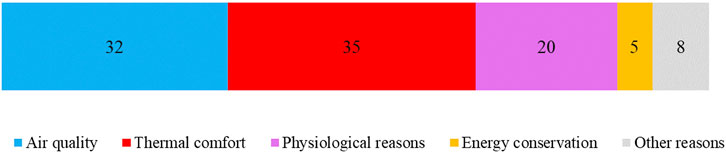
FIGURE 7. Analysis of the reasons why occupants open windows.

The results depicted in Figure 7 also show that energy conservation or energy savings ranked as fourth in this survey with 5% responses. This suggests that energy saving does not play a very important role in the occupant’s decision-making process when it comes to keeping windows open or closed. Details of the survey can be found in the Appendix.

Effects of Window Status on Indoor Air Quality

Figure 8 shows the effects of window status on indoor PM_2.5 and CO₂ concentrations. When outdoor air was polluted, the median of I/O and E-index were much higher. Although the I/O ratio is higher due to equilibrium between indoor and outdoor conditions, E-index is important to show if those levels have impact on occupant’s health. Desired building operation would be to have the I/O ratio ∼1, indicating that windows are open and outdoor air is entering indoor environment but keeping E-index < 1 suggesting that air is clean. During the wildfire period, although the windows were kept closed, the median I/O (about 0.48) and median E-index (about 1.1) were much higher than those of non-wildfire periods with open and closed windows. The median I/O ratio and E-index were both close to 0.1 during the non-wildfire period. CO₂ concentration varied with the occupancy of the rooms but did not change significantly with the window status. During the non-wildfire period, CO₂ was 424 and 428°ppm when windows were closed and open, while it grew slightly to 453°ppm when there were wildfires outside the building. During the wildfires, although the windows were closed, only partial occupancy was in the building. To this end, the CO₂ concentrations were similar to those during the open-window periods.

FIGURE 8

FIGURE 8. Window status and indoor PM_2.5 and CO₂ concentrations.

Figure 9 shows the hourly deviation between the room-level PM_2.5 and CO₂ and the building-level median values. Both during the wildfire period and the non-fire period, the PM_2.5 and CO₂ deviations were around 0, and they all have very small quartile numbers, indicating that the difference between the median of each room and the median of the whole building was very small. Given this, every room can be used as a partial study of the whole.

FIGURE 9

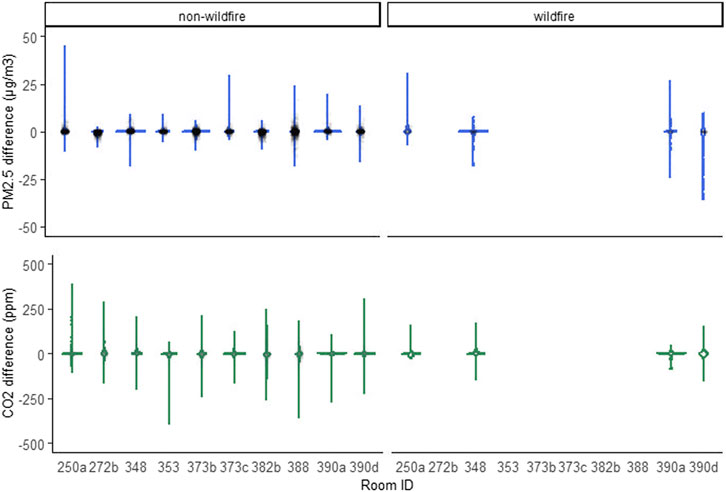
FIGURE 9. Hourly room PM_2.5 and CO₂ deviation from the building-level median.

Comparison Between Building-Scale and Urban-Scale Environmental Measurements Over a Year

Figure 10 shows the comparison of outdoor temperature, wind speed, and PM_2.5 concentration at different weather stations from January 2019 to January 2020. For outdoor temperature, the variation and the distribution are similar from three weather stations. For wind speed, the violin plot shows that the three weather stations had approximately the same temperature distribution with similar medians. The p values from Wilcoxon tests show no significant difference among weather stations. For outdoor PM_2.5 concentration, data from three weather stations are close to each other, and the outdoor PM_2.5 concentration measured at the top of Wurster Hall (the case building) was almost the same as those from the three weather stations, all in a very low level. Overall, it can be seen that outdoor temperature, wind speed, and PM_2.5 concentration from different weather stations show little difference.

FIGURE 10

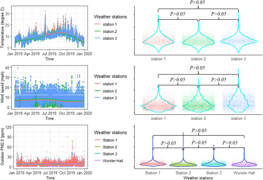
FIGURE 10. Comparison of outdoor temperature and PM_2.5 concentration at different weather stations. p values were calculated using the two-sided Wilcoxon rank-sum test. Wurster Hall is the case building.

Discussion

NV Evaluation

Figure 11 shows the NV potential index throughout the study period. The red color represents periods when outdoor PM_2.5 pollution was above 25 μg/m³, periods caused by episodic events like the wildfire. The blue and brown colors represent cold and hot outdoor conditions, respectively. The gray color marks periods when mean outdoor wind speed is higher than the upper limit calculated using Eq. 5. The green color depicts periods when outdoor conditions are favorable and NV potential is available. Results show that the high outdoor PM_2.5 concentrations mostly occurred during the hot and dry seasons, usually from August to November. The hot outdoor temperatures mainly occurred from August to October, while the cold outdoor conditions mostly happened from November to March of the next calendar year. Throughout the year of 2019, 5,075 h out of 8,287 h (with valid data), resulting in 61.2% of time, were favorable for the use on NV.

FIGURE 11

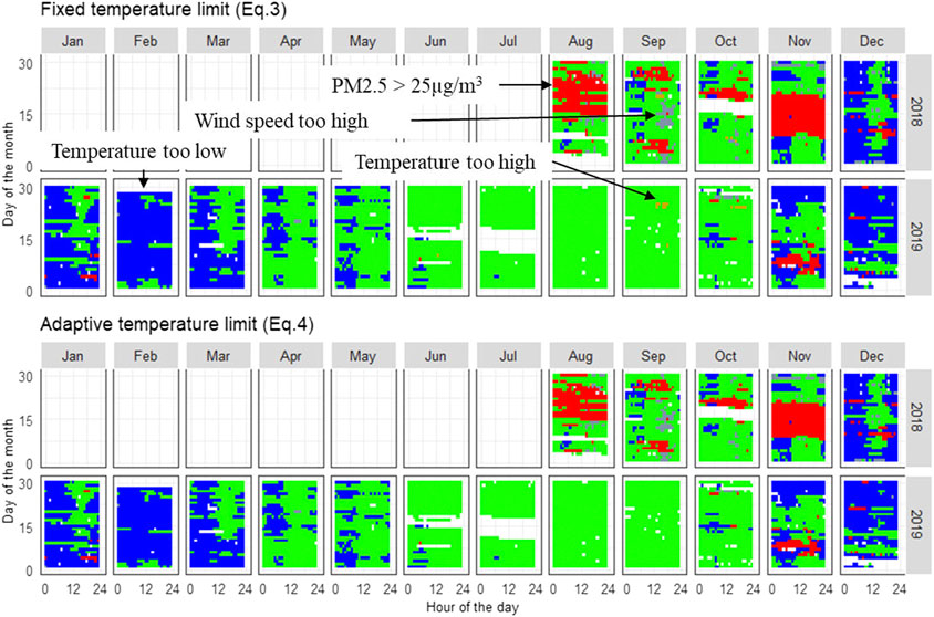
FIGURE 11. NV availability according to Eq. 3(upper row) and Eq. 4(bottom row). Red color represents that PM_2.5 concentration is higher than 25 μg/m³. Brown color represents that outdoor temperature is higher than the upper limit. Blue color represents that outdoor temperature is lower than the lower limit. Gray color represents that outdoor wind speed is too strong for NV. Green color represents that the outdoor climate condition and pollution level are favorable for the use on NV.

Table 2 compares the potential NV availability and the actual window opening hours in typical rooms. There is a huge gap between the actual NV usage and the potential availability. Even using the more conservative method (Eq. 3), the actual usage rate was less than 34.5%. This significant gap can be attributed to the occupant’s behavior. In an earlier study, Gao et al. (2014) showed that indoor conditions are better when manually opening windows is replaced with automatic window opening. A breakdown of the multiple motives for opening the windows is shown in Figure 7. Opening the windows or keeping them closed was always based on the occupant’s perception of conditions and without knowing if conditions outside are suitable for utilization of NV or if indoor conditions can be improved with the use of NV. Informing occupants that NV is available and should be used can potentially reduce the gap between actual NV use and available potential. A previous work that focused on CO₂ and classroom pointed out that visual signals were effective means of increasing NV use (Wargocki, 2015).

TABLE 2

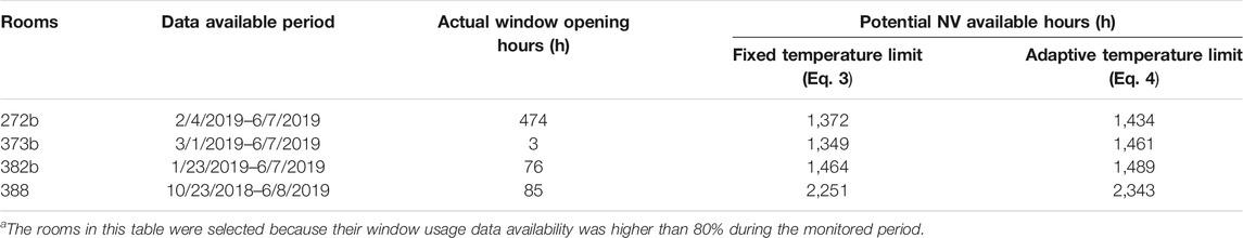
TABLE 2. Potential NV availability and actual window opening hours in typical rooms^a.

Figure 12 takes room 272 (a classroom) as an example to show the actual NV usage. It can be seen that occupants in that room frequently interacted (open/close) with the windows. From February to May, the windows were frequently opened to take advantage of the NV when the room was occupied. The indoor CO₂ and PM_2.5 were very low during the measured period. CO₂ was typically below 600 ppm, while the PM_2.5 was below 25 μg/m³.

FIGURE 12

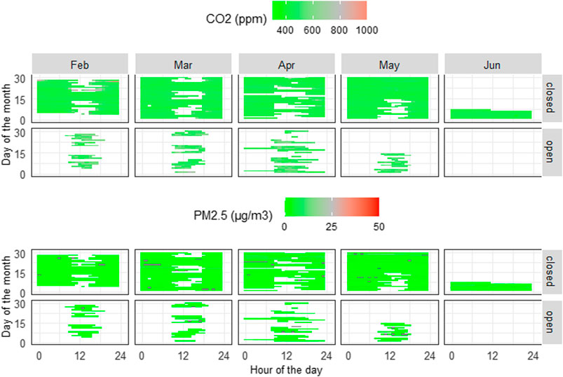
FIGURE 12. NV example: room 272.

Limitations of This Study

This study shows how to integrate indoor and outdoor information to better describe building operation. Previously, the study by Pantelic et al. (2019) demonstrated how IoT sensing can be used to describe building resilience to episodical pollution events. The current study builds on that knowledge and extends it to demonstrate how environmental and occupant behavioral data can be combined and quantify available natural potential and level of utilization of the potential. Results in this study indicate that IoT sensing information needs to be communicated with the building occupants to improve their use of NV. This is a new and largely unexplored field. When doing this, there are some limitations that could be noteworthy for future studies. First, the percentage of missing data in this study (Table 1) is relatively high for quantifying the window usage and indoor air quality throughout the year. Second, if the outdoor weather conditions, including outdoor temperature, relative humidity, wind speed, and direction can be monitored, they could provide useful information when comparing with nearby weather stations. The current study used information from the weather station 5 km away from the buildings and omitted the microclimate effects which may induce errors. Third, there are other important factors that can influence the NV availability. For example, humidity can affect the building occupant’s perception, changing their sense of a comfortable temperature range (Zhang et al., 2014). In addition to PM_2.5, nitrogen dioxide (NO₂) can be a major air pollution source that affects the NV usage, particularly in areas that are close to major roads (Zhang and Batterman, 2013).

Conclusion

Previous studies have shown that air temperature or air pollution level are limiting factors, reducing available NV potential compared to the theoretical level. This study employed a combination of an IoT environmental sensing network monitoring indoor and outdoor climate (temperature and wind speed), air pollution level (PM_2.5 and CO₂ concentrations), and window use behaviors (open and closed status) throughout the year. Indexes have been applied to evaluate the indoor air quality and NV usage potential of the buildings on different temporal and spatial scales and during episodic pollution events. The following findings are noteworthy:

1) With the help of an IoT sensor network, an NV availability tool with consideration of outdoor temperature, wind speed, and outdoor PM_2.5 concentrations was applied in the case building located in Berkeley, California. The tool can identify when the conditions are favorable for NV use and visualize the unfavorable factors via color variance.

2) By applying the NV potential index to the case building, 61.2% of time throughout the year of 2019 was determined to be favorable for NV usage. However, its actual NV usage was much less (<35%) than the potential availability. This suggests that human behavior is responsible for the gap and represents additional factors that should be considered when the NV strategy is planned and designed.

3) The actual window usage behavior (open/closed status) was significantly affected by outdoor climate condition and air pollution levels. Occupants tend to open windows when outdoor temperature is comfortable (neutral to warm) and air pollution is low.

Data Availability Statement

The raw data supporting the conclusions of this article will be made available by the authors, without undue reservation.

Ethics Statement

The studies involving human participants were reviewed and approved by UC Berkeley. The patients/participants provided their written informed consent to participate in this study.

Author Contributions

ML: data analysis, writing, and revising the manuscript; YH: data analysis and writing the manuscript; JP: conceptualizing the study, data collection, and reviewing the manuscript.

Conflict of Interest

The authors declare that the research was conducted in the absence of any commercial or financial relationships that could be construed as a potential conflict of interest.

Publisher’s Note

All claims expressed in this article are solely those of the authors and do not necessarily represent those of their affiliated organizations, or those of the publisher, the editors and the reviewers. Any product that may be evaluated in this article, or claim that may be made by its manufacturer, is not guaranteed or endorsed by the publisher.

Acknowledgments

This study was funded by CITRIS and Banatao Institute under 2018 CITRIS Seed Funding Program Award. We would also like to thank Sean Wihera from Clarity.io and Julien Stamatakis from Sensware Inc. for their valuable inputs on IoT sensing.

References

Asfour, O. (2015). Natural Ventilation in Buildings: An Overview. New York, NY: NOVA Publication, 1–25.

ASHRAE Standard 55-2013 Thermal Environmental Conditions for Human Occupancy (ANSI Approved) (2013). MADCAD.Com, (n.d.). Available at: http://www.madcad.com/store/subscription/ASHRAE-Standard-55-2013?landing=1 (Accessed September 12, 2017).

Google Scholar

Chen, Y., Tong, Z., and Malkawi, A. (2017). Investigating Natural Ventilation Potentials across the Globe: Regional and Climatic Variations. Building Environ. 122, 386–396. doi:10.1016/j.buildenv.2017.06.026

CrossRef Full Text | Google Scholar

Commission, E. (2010). Directive 2010/31/EU of the European Parliament and of the Council of 19 May 2010 on the Energy Performance of Buildings. Off. J. Eur. Union, 13–35. doi:10.2833/281509

Google Scholar

Costanzo, V., Yao, R., Xu, T., Xiong, J., Zhang, Q., and Li, B. (2019). Natural Ventilation Potential for Residential Buildings in a Densely Built-Up and Highly Polluted Environment. A Case Study. Renew. Energ. 138, 340–353. doi:10.1016/j.renene.2019.01.111

CrossRef Full Text | Google Scholar

da Graça, G. C., Linden, P., and Haves, P. (2004). Design and Testing of a Control Strategy for a Large, Naturally Ventilated Office Building. Building Serv. Eng. Res. Tech. 25, 223–239. doi:10.1191/0143624404bt107oa

CrossRef Full Text | Google Scholar

de Dear, R. J., and Brager, G. S. (2002). Thermal Comfort in Naturally Ventilated Buildings: Revisions to ASHRAE Standard 55. Energy and Buildings 34, 549–561. doi:10.1016/s0378-7788(02)00005-1

CrossRef Full Text | Google Scholar

Dutton, S. M., Banks, D., Brunswick, S. L., and Fisk, W. J. (2013). Health and Economic Implications of Natural Ventilation in California Offices. Building Environ. 67, 34–45. doi:10.1016/j.buildenv.2013.05.002

CrossRef Full Text | Google Scholar

EIA (2021). Annual Energy Outlook 2017. Available at: https://www.eia.gov/outlooks/aeo/ (Accessed September 12, 2017).

Google Scholar

Fenger, J. (2009). Air Pollution in the Last 50 Years - from Local to Global. Atmos. Environ. 43, 13–22. doi:10.1016/j.atmosenv.2008.09.061

CrossRef Full Text | Google Scholar

Gao, J., Wargocki, P., and Wang, Y. (2014). Ventilation System Type, Classroom Environmental Quality and Pupils' Perceptions and Symptoms. Building Environ. 75, 46–57. doi:10.1016/j.buildenv.2014.01.015

CrossRef Full Text | Google Scholar

Herkel, S., Knapp, U., and Pfafferott, J. (2008). Towards a Model of User Behaviour Regarding the Manual Control of Windows in Office Buildings. Building Environ. 43, 588–600. doi:10.1016/j.buildenv.2006.06.031

CrossRef Full Text | Google Scholar

Luo, M., Cao, B., Damiens, J., Lin, B., and Zhu, Y. (2015). Evaluating Thermal Comfort in Mixed-Mode Buildings: A Field Study in a Subtropical Climate. Building Environ. 88, 46–54. doi:10.1016/j.buildenv.2014.06.019

CrossRef Full Text | Google Scholar

Martins, N. R., and Carrilho da Graça, G. (2017). Impact of Outdoor PM2.5 on Natural Ventilation Usability in California's Nondomestic Buildings. Appl. Energ. 189, 711–724. doi:10.1016/j.apenergy.2016.12.103

CrossRef Full Text | Google Scholar

Morawska, L., Thai, P. K., Liu, X., Asumadu-Sakyi, A., Ayoko, G., Bartonova, A., et al. (2018). Applications of Low-Cost Sensing Technologies for Air Quality Monitoring and Exposure Assessment: How Far Have They Gone?. Environ. Int. 116, 286–299. doi:10.1016/j.envint.2018.04.018

PubMed Abstract | CrossRef Full Text | Google Scholar

Nicol, J. F., and Humphreys, M. A. (2001). A Stochastic Approach to Thermal Comfort-Occupant Behavior and Energy Use in Buildings/DISCUSSION - ProQuest, (n.d). Available at: https://search.proquest.com/docview/192502303?pq-origsite=gscholar&fromopenview=true (Accessed July 25, 2020).

Google Scholar

Oropeza-Perez, I., and Østergaard, P. A. (2014). Potential of Natural Ventilation in Temperate Countries - A Case Study of Denmark. Appl. Energ. 114, 520–530. doi:10.1016/j.apenergy.2013.10.008

CrossRef Full Text | Google Scholar

Pantelic, J., Dawe, M., and Licina, D. (2019). Use of IoT Sensing and Occupant Surveys for Determining the Resilience of Buildings to Forest Fire Generated PM2.5. PLOS ONE 14, e0223136. doi:10.1371/journal.pone.0223136

PubMed Abstract | CrossRef Full Text | Google Scholar

Parkinson, T., Parkinson, A., and de Dear, R. (2019). Continuous IEQ Monitoring System: Context and Development. Building Environ. 149, 15–25. doi:10.1016/j.buildenv.2018.12.010

CrossRef Full Text | Google Scholar

Phaff, J., de Gids, W., Ton, J., van der Ree, D., and Schijndel, L. (1980). The Ventilation of Buildings: Investigation of the Consequences of Opening One Window on the Internal Climate of a Room. Delft, Netherlands: TNO Institute for Environmental Hygiene and Health Technology (IMG-TNO).

The R Foundation (2021). R: The R Project for Statistical Computing. Available at: https://www.r-project.org/ (Accessed July 24, 2020).

Google Scholar

Raja, I. A., Nicol, J. F., McCartney, K. J., and Humphreys, M. A. (2001). Thermal Comfort: Use of Controls in Naturally Ventilated Buildings. Energy Buildings 33, 235–244. doi:10.1016/s0378-7788(00)00087-6

CrossRef Full Text | Google Scholar

Talbott, E. O., Arena, V. C., Rager, J. R., Clougherty, J. E., Michanowicz, D. R., Sharma, R. K., et al. (2015). Fine Particulate Matter and the Risk of Autism Spectrum Disorder. Environ. Res. 140, 414–420. doi:10.1016/j.envres.2015.04.021

PubMed Abstract | CrossRef Full Text | Google Scholar

Wargocki, P., and Da Silva, N. A. F. (2015). Use of Visual CO2 Feedback as a Retrofit Solution for Improving Classroom Air Quality. Indoor Air 25, 105–114. doi:10.1111/ina.12119

PubMed Abstract | CrossRef Full Text | Google Scholar

WHO Regional Office for Europe (2013). Review of Evidence on Health Aspects of Air Pollution – REVIHAAP Project: Technical Report. Copenhagen, Denmark: WHO Regional Office for Europe. Available at: http://www.ncbi.nlm.nih.gov/books/NBK361805/ (Accessed July 21, 2020).

Xiong, W., Wang, Y., Mathiesen, B. V., Lund, H., and Zhang, X. (2015). Heat Roadmap china: New Heat Strategy to Reduce Energy Consumption towards 2030. Energy 81, 274–285. doi:10.1016/j.energy.2014.12.039

CrossRef Full Text | Google Scholar

Yin, W., Zhang, G., Yang, W., and Wang, X. (2010). Natural Ventilation Potential Model Considering Solution Multiplicity, Window Opening Percentage, Air Velocity and Humidity in China. Building Environ. 45, 338–344. doi:10.1016/j.buildenv.2009.06.012

CrossRef Full Text | Google Scholar

Zhang, K., and Batterman, S. (2013). Air Pollution and Health Risks Due to Vehicle Traffic. Sci. Total Environ. 450-451, 307–316. doi:10.1016/j.scitotenv.2013.01.074

PubMed Abstract | CrossRef Full Text | Google Scholar

Zhang, K., Li, Y., Schwartz, J. D., and O׳Neill, M. S. (2014). What Weather Variables Are Important in Predicting Heat-Related Mortality? A New Application of Statistical Learning Methods. Environ. Res. 132, 350–359. doi:10.1016/j.envres.2014.04.004

PubMed Abstract | CrossRef Full Text | Google Scholar

Zhou, J., Chen, A., Cao, Q., Yang, B., Chang, V. W.-C., and Nazaroff, W. W. (2015). Particle Exposure during the 2013 Haze in Singapore: Importance of the Built environmentParticle Exposure during the 2013 Haze in Singapore: Importance of the Built Environment. Building Environ. 93, 14–23. doi:10.1016/j.buildenv.2015.04.029

CrossRef Full Text | Google Scholar

Glossary

ATD Arizona Test Dust

CO₂ Carbon dioxide

IAQ Indoor air quality

IoT Internet of Thing

HVAC Heating, ventilation, and air-conditioning

NO2 Nitrogen dioxide

NV Naturally ventilated buildings

WHO the World Health Organization

EPA Environmental Protection Agency

I/O Indoor/outdoor ratio

E index Exceedance index

PM_2.5 Particulate matter that have a diameter <2.5 µm

${\text{C}}_{{\text{measured PM}}_{2.5}}$ Measured PM_2.5 concentration (µg/m3)

Cin(t) Hourly mean indoor PM_2.5 concentration (µg/m3)

Cout(t) Hourly mean outdoor PM_2.5 concentration (µg/m3)

${\text{u}}_{\text{in},\text{max}}$ The maximum allowable indoor air speed (m/s)

${\text{u}}_{\text{out},\text{max}}$ The maximum allowable outdoor air speed (m/s)

${\text{C}}_1$ Wind speed coefficient

${\text{C}}_2$ Buoyancy coefficient (m·s−2·K−1)

${\text{C}}_3$ Turbulence coefficient (m²·s−2)

T_up Upper temperature limit (^oC)

T_low Lower temperature limit (^oC)

$\Delta {\text{T}}_{\text{max}}$ Maximum difference between indoor and outdoor temperatures (^oC)