 Erik Mitz1
 Peleg Kremer
 Justin D. Stewart
- 1Department of Political Science, Villanova University, Villanova, PA, United States
- 2Department of Geography and the Environment, Villanova University, Villanova, PA, United States
- 3Institute of Geography, Humboldt Universität zu Berlin, Berlin, Germany
Discerning the relationship between urban structure and function is crucial for sustainable city planning and requires examination of how components in urban systems are organized in three-dimensional space. The Structure of Urban Landscape (STURLA) classification accounts for the compositional complexity of urban landcover structures including the built and natural environment. Building on previous research, we develop a STURLA classification for Philadelphia, PA and study the relationship between urban structure and land surface temperature. We evaluate the results in Philadelphia as compared to previous case studies in Berlin, Germany and New York City, United States. In Philadelphia, STURLA classes hosted ST that were unique and significantly different as compared to all other classes. We find a similar distribution of STURLA class composition across the three cities, though NYC and Berlin showed strong correlation with each other but not with Philadelphia. Our research highlights the use of STURLA classification to capture a physical property of the urban landscape
Introduction
Urban spatial structure is important to understanding social and ecological interactions between the built and natural environment and provides a bridge to sustainable development (Zhou et al., 2017). Characteristics including vegetation and other landcover classes influence, and can be used to estimate ecological functions (van Oudenhoven et al., 2012; Bastian et al., 2014) and forecast changes(Dietze et al., 2018; Dietze, 2019) that are crucial under global change scenarios. Identifying patterns and processes of the structure-function relationship in the urban landscape in the context of environmental and ecological processes is challenging due to variable density and patchy spatial patterns (Pickett and Cadenasso, 2008).
While it is well established that urban areas host ecological communities subject to unique stressors (Jones and Harrison, 2004; Reese et al., 2016; Joyner et al., 2019) absent in natural systems (e.g., pollution, high population density), the influence of landscape heterogeneity on the environment is poorly described. Functional classification of urban structure is necessary for understanding the nature of social and ecological relationships in urban areas (Cadenasso et al., 2007; Zhou et al., 2014; McPhearson et al., 2016). Over the last decade, fine-scale landcover classification for urban areas have been developed (MacFaden et al., 2012; Pickard et al., 2015) that allows more nuanced analyses of urban landcover. While some functional classification approaches have been suggested (see for example Cadenasso et al., 2007), major challenges remain in integration of spatial structure and configuration that allows scalable and reproducible analysis of relationships between urban form and process.
A major barrier for understanding the relationship between urban structure and environmental function is the lack of independent measurement of the fine-scale spatial variability of the distribution of environmental and ecological variables. Particularly important is the vertical dimension (e.g., building height) and variation of the three-dimensional landscape that is rarely addressed (Alavipanah et al., 2017) in ecological studies. Where independent measurements exist, such as data from Environmental Protection Agency (EPA) air pollution monitoring stations or United States Geographical Survey (USGS) water monitoring sites, the spatial distribution is not sufficient to allow intra-urban analysis. We employ surface temperature (ST) as a proxy for a wide range of potential variables of interest across biotic and abiotic dimensions. ST is one example of a physical property of the urban environment that has been used in research addressing landcover (Zhou et al., 2011), urban heat islands (Rosenzweig et al., 2009; Zhao et al., 2011), and ecosystem services (Schwarz et al., 2011). Likewise, ST have been linked to patterns of taxonomic and functional biodiversity (Zogg et al., 1997; Scherrer and Körner, 2011). Heterogenous distributions of urban ST creates spatially distinct niches for organisms to live and or preform ecosystem functions such as soil respiration (Lloyd and Taylor, 1994). Variation in hydrology (Reyes et al., 2018), air quality (Sillman and Samson, 1995; Li et al., 2018), and social variables relevant for studies of environmental injustice (Huang and Cadenasso, 2016; Zhang et al., 2017) are also associated with changes in ST.
To account for the heterogenous vertical dimension of the built enviroment in urban lanscscape, we employ The STructure of URban Landscapes (STURLA) classification (Hamstead et al., 2016). STURLA is a supervised classification of the urban landscape into discrete countable 120 m2 units that incorporates the complexity of urban land cover structures, including the vertical dimensions of the built environment. STURLA represents urban structure underlined by the composition of eight landcover and building type classes: trees, grass\shrub, bare soil, water, low-rise buildings, mid-rise buildings, high rise buildings and other paved surfaces. While other urban classification methods such as Local Climate Zones (LCZs) (Stewart and Oke, 2012) capture patterns in surface temperature, they use pre-determined classes that may fall short of describing the highly heterogenous nature of the urban environment. The novelty in the STURLA approach is that it offers an automated composite functional classification of urban structure, including the vertical dimension, and thus can be applied to wide geographic regions systematically. STURLA has has been used to identified patterns of microbial biogeography in the atmosphere of Philadelphia (Stewart et al., 2021), and ST in NYC (Hamstead et al., 2016) and Berlin (Kremer et al., 2018).
The objectives of this short study are to identify if STURLA could explain the variation of urban structure in a new model city (Philadelphia), and quantify this variation using a physical property of the environment (ST). Results suggest STURLA identifies common urban structure units that encompass the majority of the variation in the urban landscape structure. Moreover, when correlated to surface temperature, these common urban structure classifications exhibit distinct temperature signatures for different urban structure units with temperature trends dramatically similar between Berlin and NYC. Here, we contribute to the developing literature on the urban structure-function relationship using STURLA in Philadelphia.
Materials and Methods
Study Area
Philadelphia PA, United States is the sixth largest city in the United States with a city population of 1.6 million inhabitants (U.S. Census Bureau, 2016) and hosts an average population density of 30,297 inhabitants per square kilometer. It is located at the confluence of the Delaware and Schuylkill Rivers on the eastern border of Pennsylvania with the Appalachian Mountains to the west and the Atlantic Ocean to the east. The city has a total area of about 370 km2 of which 350 km2 are land and the rest being water. Phildelphia is one of the poorest cities in the United States, with 26% of its population living in poverty (PEW, 2017). Philadelphia is also one of the most segregated cities in the United States, with African American and Asian populations concentrated in neighborhoods in West and North Philadelphia respectively (The Brookings Institution, 2003). The city’s population peaked in 1950 with over 2 million people, and was declining until 2010 when is started growing again. Recently, Philadelphia is experiencing strong, yet uneven economic resurgence reflected in job growth and rising housing prices (PEW, 2017).
Philadelphia’s urban structure emerged through the evolution of its original plan, laid out by William Penn in 1,643. It has a gridded layout with mostly low and mid-rise residential buildings. A long time “gentleman’s agreement” kept Penn’s statue on top of city hall as the highest building in the city, preventing high-rise development for decades until the 1980s. Thus, the most common residential structures in the city are rowhouses. Rowhouses commonly occupy a narrow street frontage and are attached to other homes on both sides (Simmons Schade et al., 2008). Aside from the built environment, green space in the city includes 19% tree cover and 24% grass-shrub cover that are distributed unevenly across the city with some neighborhoods densely vegetated and others with little to no green space (O’Neil-Dunne, 2011). Part of the city’s sustainability plan, Greenworks Philadelphia, includes a goal of tree canopy cover of 30% in all city neighborhoods by 2025 (City of Philadelphia, 2015a). However, until recently, the only publicly available data for a comprehensive analysis of the city’s green space has been the National Landuse-Landcover (NLCD) datasets that do not have the spatial resolution and functional categories required to identify small and fragmented patches of landscape elements within the city. In 2011, a fine scale dataset of Philadelphia landcover was released (City of Philadelphia, 2011) that is used here as the basis for the STURLA classification system. Empirical evidence from two cities, Berlin and New York City (NYC), were compared (Larondelle et al., 2014) and more detailed analysis of within class and neighborhood effects were performed in a Berlin case study (Kremer et al., 2018).
Pre-processing urban landscape structure data
To construct the urban structure dataset, we used a 2008 1.0-meter resolution land cover dataset (City of Philadelphia, 2011), the Property Assessment dataset from the Philadelphia Office of Property Assessment (City of Philadelphia, 2015b) indicating number of floors in buildings for each tax lot in the city in tabular format, and the Philadelphia Department of Water parcels dataset. We joined the property assessment tabular data to the parcels dataset using unique parcel IDs and created a 1.0-meter resolution raster dataset from the “Number of Floors” field in the Property Assessment dataset. Number of floors was classified into three categories: lowrise (1–3 stories), midrise (4–9 stories) and highrise (>9 stories) (Stewart and Oke, 2012; Larondelle et al., 2014). We then combined it with the land cover raster dataset, by replacing all building land cover pixels with a value representing building height category to create our basic urban structure dataset.
Constructing the STURLA Classification
We constructed a 120.0 m2 cellular grid aligned to the Landsat surface temperature dataset and derived STURLA classes as the presence of all land cover and building height types that fell within each grid cell. Following Hamstead et al. (2016) a zonal statistics tabulate area operation to compute the area of each land cover or building height category within each cell was conducted. Finally, we generated and assigned a STURLA class for each grid cell. For example, if a STURLA cell contains any number of pixels of trees, grass, paved, and low-rise buildings it is assigned the STURLA class “tgpl”.
Comparison of STURLA classification results from current and previous studies
Differences between cities in STURLA classes were tested statistically using permutational t-tests with Bonferroni correction (to limit the effect of multiple comparisons). The permutational t-test selected because we test data representing the population rather than a sample. The null hypothesis of the permutational t-test is that STURLA class composition does not differ between the cities. Permutational Pearson correlations were conducted to determine if the cities distribution of STURLA classes were similar between cities. These tests were conducted in R (3.6) using the package “RVAideMemoire” (Hervé, 2020).
Surface Temperature Processing
Surface temperature was obtained from Landsat seven thermal band 6(1). We obtained monthly composite data for the month of July 2010 from the Global Web-enables Landsat Data (WELD) website. We chose this month as a representative summer month based on data availability and quality. An average of scenes from one summer month were chosen to avoid any one-day outliers and to compensate for any missing data in Landsat seven scenes. Each monthly composite image is normally a composite of two Landsat scenes because LANDSAT returns to any single location every 16 days. Using a composite scene helps address the Landsat seven scan line corrector error. WELD data is terrain-corrected and radiometrically calibrated Landsat data (Roy et al., 2010). Top-of-the-Atmosphere reflectance was converted to surface temperature followed the methodology detailed in Kremer et al. (2018) in processing surface temperature.
Analysis of Class Surface Temperature
We computed the mean, min, max and standard deviation of surface temperature pixels that fell within each cell of the STURLA grid using zonal statistics (Table 1) and joined these results with the STURLA class variable. Averaging was necessary because Landsat seven thermal bands are resampled to 30 m for distribution (Roy et al., 2010) while the STURLA grid is 120 m. Thus, we averaged sixteen 30 m pixels that fell within each 120 m cell. Similar to Hamstead et al. (2016) and Larondelle et al. (2014) we focused the class temperature analysis on the most frequently occurring classes, which cumulatively comprise 90% of the city’s land area. As done with comparison of STURLA classes between cities, permutational t-tests with Bonferroni correction were employed to test significance. Likewise, the null hypothesis of the permutational t-test is that ST does not differ between the STURLA classes.
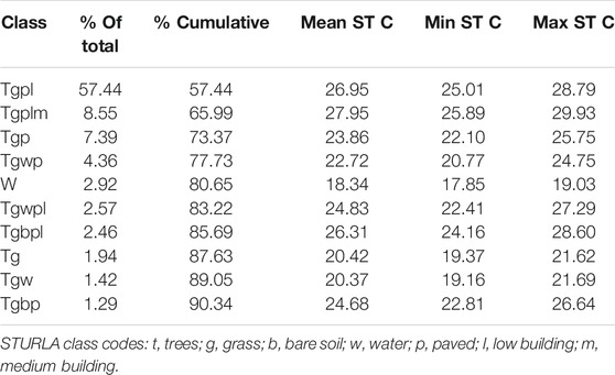
TABLE 1. 10 most common STURLA classes in Philadelphia and their ST statistics.
Results
Out of the 255 possible STURLA classes, 80 are found in Philadelphia. The most prevalent composite class in Philadelphia contains trees, grass, paved surfaces, and low-rise buildings (“tgpl”) (Table 1). The “tgpl” class accounts for about 57% of total city area and can be found in all parts of the city and was largely homogenous in spatial distribution (Figure 1A). The second largest class, “tgplm” at 8.5% of the area, which is similar to “tgpl” except it includes midrise buildings, is concentrated in the center of the city and along a few main corridors to the North and West. STURLA classes were able to identify the role of urban structure influencing ST (Figure 1B). Classes generally hosted ST that were unique (Figure 1B) and significantly different (Table 2) compared to all other classes with the exception of class “tgbp” with hosting similar ST values to “tgwp” and “tgwpl”.
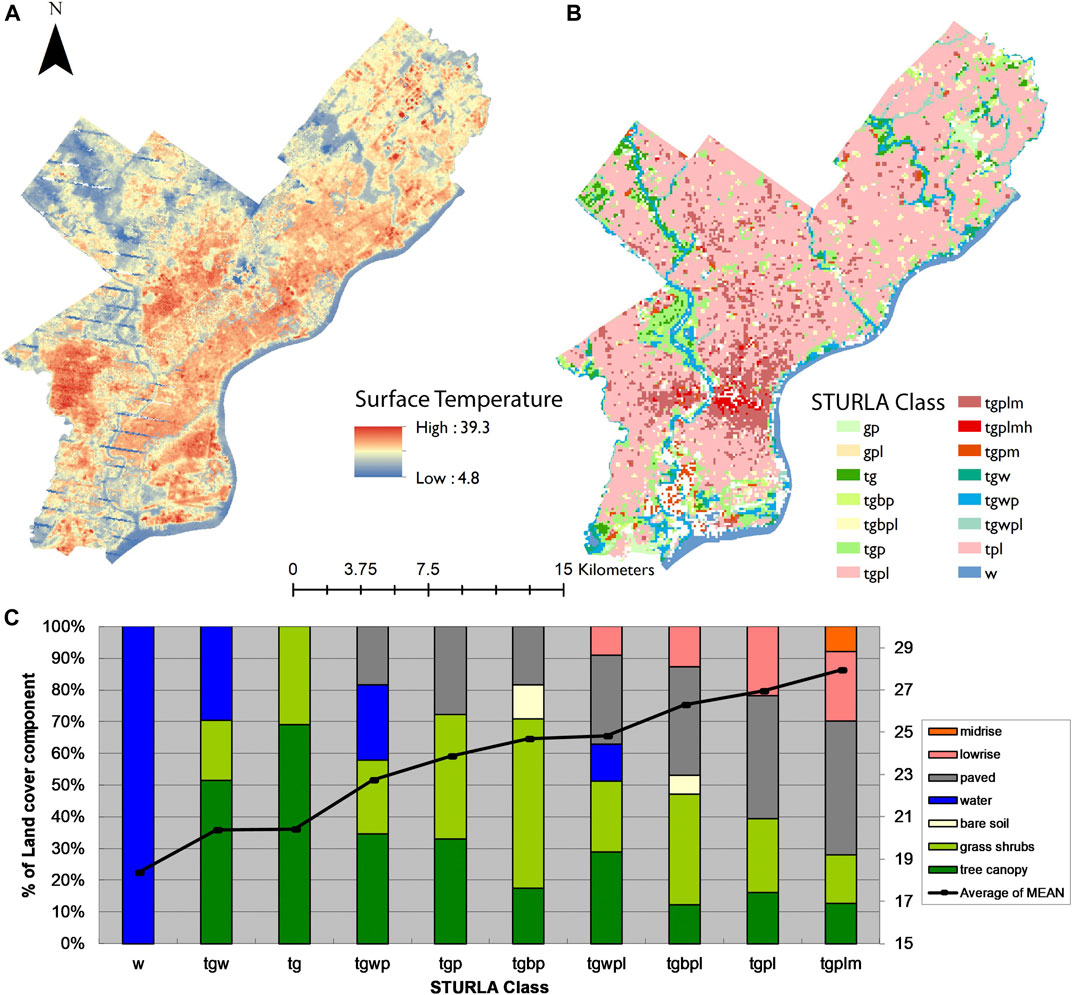
FIGURE 1. (A). Spatial distribution of STURLA classes (B). Spatial distribution of ST in Philadelphia. (C). STURLA classes, mean % landcover of individual components, and mean ST for Philadelphia. STURLA class codes: t-trees; g-grass; b-bare soil; w-water; p-paved; l-low building; m-medium buildings.
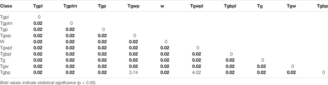
TABLE 2. p-values with Bonferroni correction from pairwise permutational t-tests (n = 999) of ST values for the top ten STURLA classes.
The prevalence and distribution of the STURLA classes in Philadelphia differs from what we found in previous studies of urban structure NYC and Berlin (Figure 2). In Berlin and NYC, ∼1/3 of the landscape can be explained by one highly composite STURLA class. Another difference between the results in Philadelphia and previous studies is the number of classes that cumulatively explain 90% of the area of the city. Ten classes covered 90% of the area of Philadelphia while the same number of classes only covered 79% of the area of New York City and 68% of the area in Berlin. Despite these differences, pairwise comparison of each city revealed that STURLA class proportions were not significantly different between the cities (all p > 0.05) Still, Berlin and NYC were highly correlated (r2 = 0.952, p < 0.05) while Philadelphia’s distribution of urban structure remained insignificantly correlated to the other cities (p > 0.05).
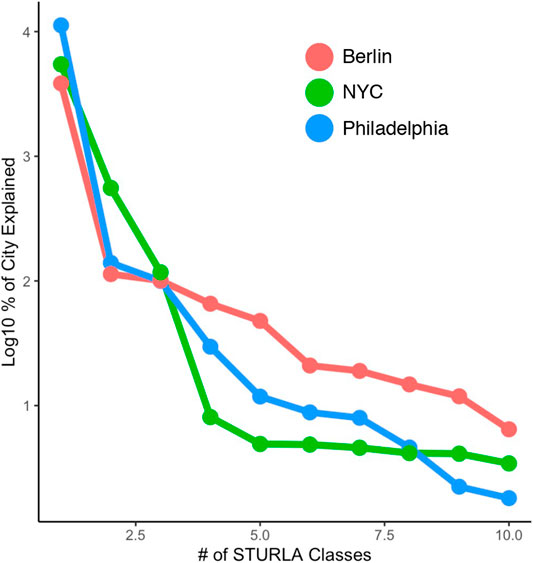
FIGURE 2. Ranked distribution plot of STURLA class frequency by log 10 class abundance for each city.
Discussion
STURLA captured urban structure and characterized the physical property of ST in Philadelphia as previously done in NYC (Hamstead et al., 2016) and Berlin (Larondelle et al., 2014; Kremer et al., 2018), despite variation in size, demography, and planning history. This suggests that urban areas may be subject to similar processes that result in between city-redundant spatial organizations (Votsis and Haavisto, 2019). STURLA offers a computationally inexpensive alternative to network analyses of urban structure (Zhong et al., 2014). In addition, STURLA may be suited for understanding urban biogeography, environmental justice, and city planning for a sustainable future. Additional city comparisons may also identify clusters of urban areas that would benefit from similar management practices.
Due to the compositional nature of a STURLA cell, the classification is subject to within class variation. Figure 3 provides an example of compositional variability in Philadelphia within the most common class in “tgpl”, using six grid cells taken from a larger city-wide random sample. The different grid cells and corresponding satellite imagery show the different types of buildings and proportion of each element of the class, trees, grass, paved surfaces, and lowrise buildings, can vary greatly from one another but still fall into the class. Most grid cells from the “tgpl” class show row houses or single-family detached houses since they fall within the size parameters of lowrise buildings (1–3 stories). Our results demonstrate that despite this variability, most classes host unique ST, suggesting that the STURLA classes are a meaningful representation of urban structure.
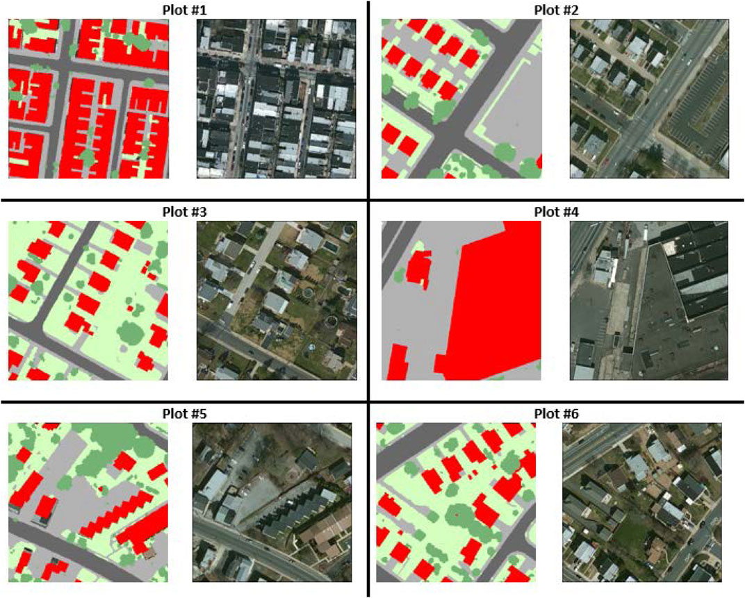
FIGURE 3. Example of the composition of STURLA grid cells of the most common STURLA class in Philadelphia “tgpl”. STURLA “tpgl” cells are shown next to corresponding areal imagery.
One limitation of the STURLA classification is the binary nature of the STURLA grid. If the STURLA grid size, location or orientation were shifted it may change the relative proportions of within class elements (e.g., trees decrease and other elements increase). Despite this limitation, STURLA classes are a discrete countable number and have a log-normal to Poisson distribution. Thus, the ranked order abundances of different STURLA classes should not vary in the most frequent classes. For example, since “tgpl” is common in Philadelphia, a reduction in a large number of “tgpl” classes in the city would be relatively less influential than additions/reductions of less common class.
Additional limitations of this study are due to data limitations of the ST dataset. Results might vary by the choice of ST temporal aggregation. Averaging a shorter or longer temporal span (e.g., one day or a season long average) could result in variation in the observed relationships. Additional research is needed to determine the sensitivity of the STURLA-ST relationship to variation in ST temporal aggregation.
Conclusion
In this paper we demonstrate the application of STURLA classification to quantify the relationship between urban structure and surface temperature in Philadelphia. We compare Philadelphia results with results from previous STURLA research in Berlin and NYC and show it can be applied to cities with different historical patterns of development in a reproducible manner. Furthermore, patterns in class abundance and composition can be used to determine the surface temperature signature of a composite landscape. Additional research is needed to compare cities of vastly different urban structure and identify patterns in the relationship between urban structure with social and ecological properties of the environment. Understanding general urban structure-environmental function relationships will help build tools for effective urban planning and management under global change scenarios.
Data Availability Statement
The raw data supporting the conclusions of this article will be made available by the authors, without undue reservation.
Author Contributions
Conceptualization, PK, NL, and EM; methodology, PK, NL, EM, and JS; formal analysis, EM and JS; data curation, PK, EM, NL, and JS; writing—original draft preparation, EM and PK; visualization, EM, NL, and JS; supervision, PK and NL. All authors have read and agreed to the published version of the manuscript.
Conflict of Interest
The authors declare that the research was conducted in the absence of any commercial or financial relationships that could be construed as a potential conflict of interest.
Acknowledgments
This work received funding from Villanova University’s Falvey Memorial Library Scholarship Open Access Reserve (SOAR) Fund.
References
Alavipanah, S., Haase, D., Lakes, T., and Qureshi, S. (2017). Integrating the third dimension into the concept of urban ecosystem services: a review. Ecol. Indic. 72, 374–398. doi:10.1016/j.ecolind.2016.08.010
Bastian, O., Grunewald, K., Syrbe, R.-U., Walz, U., and Wende, W. (2014). Landscape services: the concept and its practical relevance. Landscape Ecol. 29 (9), 1463–1479. doi:10.1007/s10980-014-0064-5
Cadenasso, M. L., Pickett, S. T. A., and Schwarz, K. (2007). Spatial heterogeneity in urban ecosystems: reconceptualizing land cover and a framework for classification. Front. Ecol. Environ. 5 (2), 80–88. doi:10.1890/1540-9295(2007)5
City of Philadelphia (2015a). Greenworks Philadelphia: 2015 progress report. Available at: https://www.phila.gov/media (Accessed May 2020).
City of Philadelphia (2015b). Property assessment data. Available at: https://property.phila.gov/ (Accessed May 2020).
City of Philadelphia (2011). Philadelphia land cover raster OpenDataPhilly. Available at: https://www.opendataphilly.org/ (Accessed May 2020).
Dietze, M. C., Fox, A., Beck-Johnson, L. M., Betancourt, J. L., Hooten, M. B., Jarnevich, C. S., et al. (2018). Iterative near-term ecological forecasting: needs, opportunities, and challenges. Proc. Natl. Acad. Sci. United States America. doi:10.1073/pnas.1710231115
Hamstead, Z. A., Kremer, P., Larondelle, N., McPhearson, T., and Haase, D. (2016). Classification of the heterogeneous structure of urban landscapes (STURLA) as an indicator of landscape function applied to surface temperature in New York City. Ecol. Indic. 70, 574–585. doi:10.1016/j.ecolind.2015.10.014
Hervé, M. (2020). Package ‘RVAideMemoire’. Available at: https://github.com/cran/RVAideMemoire (Accessed May 2020).
Huang, G., and Cadenasso, M. (2016). People, landscape, and urban heat island: dynamics among neighborhood social conditions, land cover and surface temperatures. Landscape Ecol. 31 (10), 1–9. doi:10.1007/s10980-016-0437-z
Jones, A. M., and Harrison, R. M. (2004). The effects of meteorological factors on atmospheric bioaerosol concentrations--a review. Sci. Total Environ. 326 (1), 151–180. doi:10.1016/j.scitotenv.2003.11.021
Joyner, J. L., Kerwin, J., Deeb, M., Lozefski, G., Prithiviraj, B., Paltseva, A., et al. (2019). Green infrastructure design influences communities of urban soil bacteria. Front. Microbiol. 10, 982. doi:10.3389/fmicb.2019.00982
Kremer, P., Larondelle, N., Zhang, Y., Pasles, E., and Haase, D. (2018). Within-class and neighborhood effects on the relationship between composite urban classes and surface temperature. Sustainability 10 (3), 645. doi:10.3390/su10030645
Larondelle, N., Hamstead, Z. A., Kremer, P., Haase, D., and McPhearson, T. (2014). Applying a novel urban structure classification to compare the relationships of urban structure and surface temperature in Berlin and New York City. Appl. Geogr. 53, 427–437. doi:10.1016/j.apgeog.2014.07.004
Li, H., Meier, F., Lee, X., Chakraborty, T., Liu, J., Schaap, M., et al. (2018). Interaction between urban heat island and urban pollution island during summer in Berlin. Sci. Total Environ. 636, 818–823. doi:10.1016/j.scitotenv.2018.04.254
Lloyd, J., and Taylor, J. A. (1994). On the temperature dependence of soil respiration. Funct. Ecol. doi:10.2307/2389824
MacFaden, S. W., O’Neil-Dunne, J. P. M., Royar, A. R., Lu, J. W. T., and Rundle, A. G. (2012). High-resolution tree canopy mapping for New York City using LIDAR and object-based image analysis. J. Appl. Remote Sens. 6 (1), 3567. doi:10.1117/1.JRS.6.063567
McPhearson, T., Pickett, S. T. A. A., Grimm, N. B., Niemelä, J., Alberti, M., Elmqvist, T., et al. (2016). Advancing urban ecology toward a science of cities. BioScience 66, 1–15. doi:10.1093/biosci/biw002
O’Neil-Dunne, J. (2011). A report on the city of Philadelphia’s existing and possible tree canopy. Available at: http://gis.w3.uvm.edu/utc/Reports/TreeCanopy_Report_Philadelphia.pdf (Accessed May 2020).
PEW (2017). Philadelphia 2017: The state of the city. Available at: https://www.pewtrusts.org/en/projects/philadelphia-research-and-policy-initiative/state-of-the-city (Accessed May 2020).
Pickard, B. R., Daniel, J., Mehaffey, M., Jackson, L. E., and Neale, A. (2015). EnviroAtlas: a new geospatial tool to foster ecosystem services science and resource management. Ecosystem Serv. 14, 45–55. doi:10.1016/j.ecoser.2015.04.005
Pickett, S. T. A., and Cadenasso, M. L. (2008). Linking ecological and built components of urban mosaics: an open cycle of ecological design. J. Ecol. 96, 8–12. doi:10.1111/j.1365-2745.2007.01310.x
Reese, A. T., Savage, A., Youngsteadt, E., McGuire, K. L., Koling, A., Watkins, O., et al. (2016). Urban stress is associated with variation in microbial species composition-but not richness-in Manhattan. ISME J. 10 (3), 751–760. doi:10.1038/ismej.2015.152
Reyes, B., Hogue, T., and Maxwell, R. (2018). Urban irrigation suppresses land surface temperature and changes the hydrologic regime in semi-arid regions Water 10 (1), 1563. doi:10.3390/w10111563
Rosenzweig, C., Solecki, W. D., Cox, J., Hodges, S., Parshall, L., Lynn, B., et al. (2009). Mitigating New York city’s heat island: integrating stakeholder perspectives and scientific evaluation. Bull. Am. Meteorol. Soc. 90 (9), 1297–1312. doi:10.1175/2009BAMS2308.1
Roy, D. P., Ju, J., Kline, K., Scaramuzza, P. L., Kovalskyy, V., Hansen, M., et al. (2010). Web-enabled landsat data (WELD): Landsat ETM+ composited mosaics of the conterminous United States. Remote Sens. Environ. 114 (1), 35–49. doi:10.1016/j.rse.2009.08.011
Scherrer, D., and Körner, C. (2011). Topographically controlled thermal-habitat differentiation buffers alpine plant diversity against climate warming. J. Biogeogr. 38, 406–416. doi:10.1111/j.1365-2699.2010.02407.x
Schwarz, N., Bauer, A., and Haase, D. (2011). Assessing climate impacts of planning policies—an estimation for the urban region of Leipzig (Germany). Environ. Impact Assess. Rev. 31 (2), 97–111. doi:10.1016/j.eiar.2010.02.002
Sillman, S., and Samson, P. J. (1995). Impact of temperature on oxidant photochemistry in urban polluted rural and remote environments. J. Geophys. Res. 100, 11497–11508. doi:10.1029/94jd02146
Simmons Schade, R., Architects, B., Spina, L. M., Farnham, J., Fine, A., Gallery, J. A., et al. (2008). Philadelphia rowhouse manual A practical guide for homeowners special thanks to steering committee.
Stewart, I. D., and Oke, T. R. (2012). Local climate Zones for urban temperature studies. Bull. Am. Meteorol. Soc. 93 (12), 1879–1900. doi:10.1175/BAMS-D-11-00019.1
Stewart, J. D., Kremer, P., Shakya, K. M., Conway, M., and Saad, A. (2021). Outdoor atmospheric microbial diversity is associated with urban landscape structure and differs from indoor-transit systems as revealed by mobile monitoring and three-dimensional spatial analysis. Front. Ecol. Evol. 9, 620461. doi:10.3389/fevo.2021.620461
The Brookings Institution (2003). Philadelphia in focus: a profile from census 2000. Washington, D.C.: The Brookings Institution.
van Oudenhoven, A. P. E., Petz, K., Alkemade, R., Hein, L., and de Groot, R. S. (2012). Framework for systematic indicator selection to assess effects of land management on ecosystem services. Ecol. Indic. 21, 110–122. doi:10.1016/j.ecolind.2012.01.012
Votsis, A., and Haavisto, R. (2019). Urban dna and sustainable cities: a multi-city comparison. Front. Environ. Sci. 7 (JAN), 4. doi:10.3389/fenvs.2019.00004
Zhang, X., Estoque, R. C., and Murayama, Y. (2017). An urban heat island study in Nanchang City, China based on land surface temperature and social-ecological variables. Sust. Cities Soc. 32, 557–568. doi:10.1016/j.scs.2017.05.005
Zhao, C., Fu, G., Liu, X., and Fu, F. (2011). Urban planning indicators, morphology and climate indicators: a case study for a north-south transect of Beijing, China. Building Environ. 46 (5), 1174–1183. doi:10.1016/j.buildenv.2010.12.009
Zhong, C., Arisona, S. M., Huang, X., Batty, M., and Schmitt, G. (2014). Detecting the dynamics of urban structure through spatial network analysis. Int. J. Geographical Inf. Sci. 28 (11). doi:10.1080/13658816.2014.914521
Zhou, W., Cadenasso, M., Schwarz, K., and Pickett, S. T. A. (2014). Quantifying spatial heterogeneity in urban landscapes: integrating visual interpretation and object-based classification. Remote Sensing 6 (4), 3369–3386. doi:10.3390/rs6043369
Zhou, W., Huang, G., and Cadenasso, M. L. (2011). Does spatial configuration matter? Understanding the effects of land cover pattern on land surface temperature in urban landscapes. Landscape Urban Plann. 102 (1), 54–63. doi:10.1016/j.landurbplan.2011.03.009
Zhou, W., Pickett, S. T. A., and Cadenasso, M. L. (2017). Shifting concepts of urban spatial heterogeneity and their implications for sustainability. Landscape Ecol. 32 (1), 15–30. doi:10.1007/s10980-016-0432-4
Keywords: urban landscape, urban surface temperature, STURLA, urban structure, city comparison
Citation: Mitz E, Kremer P, Larondelle N and Stewart JD (2021) Structure of Urban Landscape and Surface Temperature: A Case Study in Philadelphia, PA. Front. Environ. Sci. 9:592716. doi: 10.3389/fenvs.2021.592716
Received: 07 August 2020; Accepted: 26 January 2021;
Published: 10 March 2021.
Edited by:
Marian Stuiver, Wageningen University and Research, NetherlandsReviewed by:
Athanasios Votsis, Finnish Meteorological Institute, FinlandDamian Lowicki, Adam Mickiewicz University, Poland
Copyright © 2021 Mitz, Kremer, Larondelle and Stewart. This is an open-access article distributed under the terms of the Creative Commons Attribution License (CC BY). The use, distribution or reproduction in other forums is permitted, provided the original author(s) and the copyright owner(s) are credited and that the original publication in this journal is cited, in accordance with accepted academic practice. No use, distribution or reproduction is permitted which does not comply with these terms.
*Correspondence: Peleg Kremer, cGVsZWcua3JlbWVyQHZpbGxhbm92YS5lZHU=