
95% of researchers rate our articles as excellent or good
Learn more about the work of our research integrity team to safeguard the quality of each article we publish.
Find out more
ORIGINAL RESEARCH article
Front. Environ. Sci. , 17 February 2021
Sec. Environmental Informatics and Remote Sensing
Volume 8 - 2020 | https://doi.org/10.3389/fenvs.2020.587354
This article is part of the Research Topic Emerging Technologies and Techniques for Remote Sensing of Coastal and Inland Waters View all 14 articles
Satellite and aerial imagery have been used extensively for mapping the abundance and distribution of giant kelp (Macrocystis pyrifera) in southern California. There is now great potential for using unoccupied aerial vehicles (UAVs) to map kelp canopy at very high resolutions. However, tides and currents have been shown to affect the amount of floating kelp canopy on the water surface, and the impacts of these processes on remotely sensed kelp estimates in this region have not been fully quantified. UAVs were used to map fine-scale changes in canopy area due to tidal height and current speed at kelp forests off the coast of Palos Verdes, CA and Santa Barbara, CA. An automated method for detecting kelp canopy was developed that was 67% accurate using red-green-blue (RGB) UAV imagery and 93% accurate using multispectral UAV imagery across a range of weather, ocean, and illumination conditions. Increases in tidal height of 1 m reduced the amount of floating kelp canopy by 15% in Santa Barbara and by over 30% in Palos Verdes. The effect of current speed on visible kelp canopy was inconclusive, but there was a trend towards lower canopy area with increased current speed. Therefore, while tidal height and current speed can introduce significant variability to estimates of kelp abundance, the magnitude of this variability is site specific. Still, UAVs are a valuable tool for mapping of kelp canopy and can provide greater spatial resolution and temporal coverage than is possible from many satellite sensors. This data can provide insight into the patterns and drivers of high frequency fluctuations in kelp abundance.
Giant kelp (Macrocystis pyrifera) serves as the structural and nutritional foundation for globally distributed and highly productive nearshore ecosystems (Dugan et al., 2003; Graham et al., 2007; Miller et al., 2018). Giant kelp forests offer great societal and economic value through the support of fisheries, recreation, and a wide range of products including cosmetics, food, fertilizer, and biofuels (Gentry et al., 2017, Gentry et al., 2019). Accordingly, monitoring the abundance and distribution of this valuable resource is particularly important in the face of global climate change, as marine ecosystems are especially susceptible to the effects of climatic disturbances (Harley et al., 2006).
Fixed to subtidal, rocky reefs with a holdfast, giant kelp fronds extend vertically towards the sea surface to form dense, floating canopies, which are visible from above. Satellite imagery has shown great potential for monitoring kelp populations, as floating kelp canopies are visible with multispectral spaceborne sensors (Cavanaugh et al., 2011; Bell et al., 2015a, Bell et al., 2020; Mora-Soto et al., 2020). Repeated global measurements provide a comprehensive view of changes in kelp canopy area through time, enabling the roles of seasonal (e.g., wave disturbance and nutrient availability) to decadal scale (e.g., the El Niño-Southern Oscillation (ENSO) and the North Pacific Gyre Oscillation (NPGO)) drivers to be evaluated across a wide range of spatial scales. Satellites with moderate spatial resolution (10–30 m) can be used to accurately estimate the area and biomass of continuous kelp canopies on the order of hundreds of sq. meters in size (Cavanaugh et al., 2011), yet are unable to detect sparse stands of kelp that cover less than 15% of a pixel (i.e., 135 m2 for a 900 m2 Landsat pixel; Hamilton et al., 2020). Additionally, shallow kelp forests can be difficult to differentiate from land, especially when pixels contain a mixture of land, water, and kelp (Schroeder et al., 2019a; Bell et al., 2020; Hamilton et al., 2020). These issues limit the suitability of moderate resolution satellite imagery for monitoring giant kelp habitat in regions where kelp beds are small, sparse and/or found close to the shoreline (e.g., British Columbia; Nijland et al., 2019).
Tidal height and surface currents introduce additional complexity into aerial estimates of kelp canopy area (Britton-Simmons et al., 2008). The amount of kelp exposed on the water surface periodically fluctuates with incoming and outgoing tides. Portions of the canopy submerge and reemerge as tidal height increases and decreases, and at high tide, deeply submerged individuals become undetectable with aerial and satellite-based sensors. Similarly, strong currents can temporarily immerse floating canopies, changing the shape and coverage of the forest when viewed from above.
In southern California, satellite and aerial imagery have been used extensively for monitoring the drivers of giant kelp biomass dynamics, kelp physiological condition, and synchrony and metapopulation dynamics (Jensen et al., 1980; Deysher 1993; Stekoll et al., 2006; Cavanaugh et al., 2011; Cavanaugh et al., 2013; Cavanaugh et al., 2014; Cavanaugh et al.,2019; Bell et al., 2015a; Bell et al., 2015b; Bell et al., 2020; Castorani et al., 2015; Castorani et al., 2017). Despite this widespread use, it is unclear how tidal height and surface currents impact apparent bed size in this region. Britton-Simmons et al. (2008) demonstrated a significant impact of tides and currents on bull kelp (Nereocystis luetkeana) canopy using oblique-angle, shore-based photography, however these impacts have not been quantified for giant kelp, which has a different morphology from bull kelp. In addition, there are limitations with estimating area from oblique-angle imagery, and the sensitivity of this imagery to tides and currents may be different than that of nadir imagery.
Unoccupied aerial vehicles (UAVs) present a low-cost, versatile solution to the challenges and limitations associated with using satellite imagery to study small or sparse kelp beds. Offering spatial resolutions on the order of centimeters, UAVs not only provide the fine resolution necessary to monitor environmental processes on fine spatial scales, but they also present the flexibility in timing of image capture (Whitehead and Hugenholtz 2014; Whitehead et al., 2014). Additionally, sensor systems with varying spectral capabilities have been developed for UAV platforms, ranging from digital color cameras, containing red, green, and blue channels (RGB) to hyperspectral (Whitehead and Hugenholtz 2014). While emergent giant kelp canopy prominently reflects in the near infrared (NIR), seawater has a high absorption (Jensen et al., 1980; Schroeder et al., 2019a), and so NIR imagery is useful for detecting surface canopy (Cavanaugh et al., 2010) but has limited ability to detect subsurface kelp.
UAV imagery has been successfully implemented in the detection and mapping of both floating and submerged seaweed communities, yet sun glint, crashing waves, shadows, and spectral noise have made automated classification schemes problematic, necessitating manual image classifications (Kellaris et al., 2019; Taddia and Russo 2019; Thomsen et al., 2019). Here, we present a novel automated canopy detection algorithm that can be applied consistently to UAV imagery collected across varying conditions. We then quantify the influence of tides and currents on estimates of floating giant kelp canopy area in southern California using these methods. Using this automated detection method, we introduce field collection methods used to create a time series of kelp canopy area from multispectral UAV imagery. This dataset allows for the local scale assessment of giant kelp canopy area at 10 cm resolution every two weeks for one year while controlling for tides. The time series provides insight to patterns and drivers of high-frequency variability in giant kelp abundance in southern California.
The study area included two kelp forests located on the southern California coast: Arroyo Quemado (34°28.127′N, 120° 07.285′W) west of Santa Barbara, and Honeymoon Cove (33°45.906′N, 118° 25.392′W) at Palos Verdes (Figure 1). Both kelp forests experience tidal fluctuations ranging from∼−0.55 m to 2.2 m.
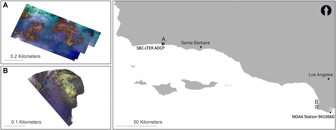
FIGURE 1. Santa Barbara, California study site: Arroyo Quemado (A) with associated SBC-LTER ADCP and Palos Verdes, California study site: Honeymoon Cove (B) with associated NOAA station 9410660.
Flights were conducted throughout the tidal range (hereafter referred to as tidal surveys) on January 2, 2018 at Arroyo Quemado (−0.52 m–2.15 m) and on July 9, 2018 (0.64 m–1.96 m) and July 18, 2018 (0.25 m–1.56 m) at Honeymoon Cove to capture the tidal responses of kelp beds with different structural properties (Supplementary Table S1). The Arroyo Quemado kelp forest is located offshore of an open coast, and one discrete stand was sampled within the forest∼400 m from the shoreline. The Honeymoon Cove kelp forest extends throughout a sheltered cove, with thicker stands of kelp fringing the coastline and sparser stands of kelp covering the rest of the cove. Flights were only conducted within the cove, but the kelp forest continuously extended past the section that was surveyed. The flight duration for each site was approximately 20–30 min. For each tidal survey, hourly flights were performed across the tidal amplitude (approximately 6 h). Wind speeds were less than 8 km/h during all tidal survey flights.
A separate series of UAV flights were conducted at Arroyo Quemado in order to isolate the effects of currents. These consisted of one flight per day at the same tidal stage (bottom of low tide) across a 5 day span (June 26, 2019 to June 30, 2019) with varying wind and current speeds (Supplementary Table S1).
A MicaSense RedEdge sensor mounted on a DJI Matrice 100 quadcopter was used to survey the kelp bed at Honeymoon Cove. The RedEdge simultaneously captures data in five spectral channels, the blue (475 nm center, 20 nm bandwidth), green (560 nm center, 20 nm bandwidth), red (668 nm center, 10 nm bandwidth), red-edge (717 nm center, 10 nm bandwidth), and NIR (840 nm center, 40 nm bandwidth). Sun angle and illumination conditions varied temporally across each survey, and while the RedEdge was equipped with a downwelling light sensor (DLS), DLS data were omitted in image processing as sensor measurements during flight vary with the pitch and roll of the UAV (Hakala et al., 2018). To calibrate reflectance for each flight, a spectral calibration panel with known reflectance was imaged before and after each flight. The along-track overlap between consecutive images was set to 80%, and the side-track overlap between consecutive flight lines was set to a minimum of 75%. Sun glint distorted the reflectance of pixels in the middle and edges of images taken when the sun was at or close to zenith. To increase pixel coverage unaffected by sun glint, the side-track overlap was increased to 85% during these flights. Due to UAV and sensor availability between collaborators, a MicaSense Altum sensor mounted on a DJI Matrice 200 quadcopter was used to survey the kelp bed at Arroyo Quemado. The Altum simultaneously captures data in five channels similar to the RedEdge, the blue (475 nm center, 32 nm bandwidth), green (560 nm center, 27 nm bandwidth), red (668 nm center, 14 nm bandwidth), red-edge (717 nm center, 13 nm bandwidth), and NIR (840 nm center, 57 nm bandwidth). All other settings remained consistent to those used with the RedEdge sensor.
A moored CTD and Acoustic Doppler Current Profiler (ADCP) from the Santa Barbara Coastal Long Term Ecological Research (SBC LTER) program (http://sbc.lternet.edu) were located within the Arroyo Quemado kelp forest, allowing for simultaneous in situ depth and current measurement comparisons with each Arroyo Quemado flight. These data included north velocity, east velocity, and water depth, which were provided in 20 min intervals. Velocity data were collected at 16 different heights in the water column, from 2.5 m to 17.5 m from the bottom. Measurements from 12.5 m readings were used for this study, as measurements taken above 12.5 m from the bottom often yielded no data values at low tide. Both depth and current measurements were linearly interpolated to one min intervals to match both the tidal height and current speed at the midpoint (from UAV launch to landing) of the time each kelp forest was imaged. NOAA/NOS/CO-OPS one min tidal measurements (https://tidesandcurrents.noaa.gov/1mindata.html) were used from Station 9410660 for simultaneous in situ depth measurement comparisons with each Honeymoon Cove flight.
Before analyzing the UAV images, raw pixel values were converted from digital numbers (DN) to reflectance using the recommended MicaSense processing steps (https://github.com/micasense/imageprocessing). A dark pixel correction was applied to reduce sensor noise, an imager specific radiometric calibration function was calculated to account for radiometric inaccuracies, vignette effects were removed from image corners, and each pixel was divided by image gain, exposure time, and a sensor-specific calibration coefficient (all imager and sensor specific calibrations were provided by MicaSense). For each band, the pixels within the inner 75% of reflectance panel images captured before and after each flight were extracted and averaged to account for any illumination changes from launch to landing. The provided Lambertian panel for the RedEdge and Altum have a known reflectance for each band, which were used to convert DN to reflectance.
Pixels altered by sun glint and crashing waves introduce distortion into individual images, as these pixels are inconsistent across space and time, making image mosaicking difficult. To reduce distortion, these pixels were masked from each band of pre-mosaicked reflectance images using gray-level co-occurrence matrices (GLCM), which have been successful in a variety of remote sensing-based classifications (Changhui et al., 2013; Huang et al., 2014; Zheng et al., 2018). GLCMs yield textural features from images by calculating the spatial distribution of the gray-level variations of individual band values (Haralick et al., 1973). The function graycomatrix in MATLAB (2018) creates a GLCM by describing pixel spatial dependency, or the frequency at which a pixel with value i occurs adjacent to a pixel with value j (MATLAB, 2018).
In the blue portion of the visible spectrum, dense kelp has a relatively low reflectance, while water has a relatively high reflectance (Supplementary Figure S1; Schroeder et al., 2019b). As a result, graycomatrix was applied to the blue band of each image to help isolate glint pixels and to reduce the potential for misclassification between glint and kelp. The brightest pixel grouping within each matrix was used to identify glint and wave pixels within all images containing 100% water. If masks were applied to images with land, this process may accidentally mask land and coastal pixels as well. A 5-pixel buffer was placed around any pixels classified as glint, and the resulting masks were exported for each individual UAV image (Figure 2).
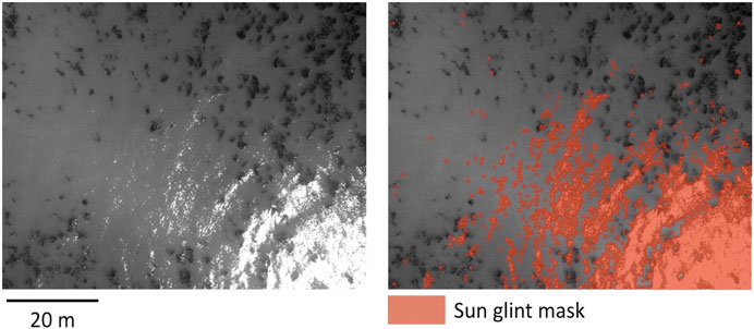
FIGURE 2. Unprocessed, grayscale UAV image (left) and corresponding sun glint mask (right). All reflectance pixels found within the sun glint mask were removed during photogrammetric processing to improve mosaicking success.
Reflectance images were mosaicked into orthomosaics using the structure from motion photogrammetric software Agisoft Metashape Pro (formerly Agisoft Photoscan Pro; Agisoft Photoscan Pro version 1.4.5 through Metashape Pro version 1.6.2 were used for processing; Agisoft, St. Petersburg, Russia). Metashape Pro allows users to directly import binary masks that are associated with raw UAV image files (i.e., Metashape will correspond images with their respective masks if the files share the same file name), and the software will exclude masked areas when finding tie points for photogrammetric stitching. As a result, only the pixels unaffected by glint will be incorporated into the final orthomosaic (Figure 3). To account for error in measurements of the UAV’s onboard GPS, each orthomosaic GeoTiff was manually georeferenced. An arbitrary UAV image from Honeymoon Cove and Arroyo Quemado were selected as the base image, and ten coordinates located along the shoreline of each site were located. All subsequent images were georeferenced to these ten points to ensure that our images were referenced to one another through time. Once images were georeferenced, they were resampled to 10 cm × 10 cm, and all land and coastal pixels within 10 m of the low-tide line were removed.
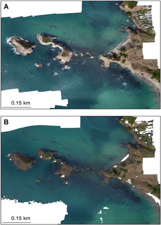
FIGURE 3. Example of a UAV-based orthomosaic export from Agisoft Metashape Pro without the glint correction applied (A) and with the glint correction applied (B). Land areas that were erroneously removed with the glint correction are apparent–masks containing coastline can be excluded to reduce this effect.
Twenty vegetation indices were compared to determine which was best at separating kelp from water in UAV imagery. These included both previously published indices as well as simple additive and multiplicative band combinations. Ten indices were restricted to RGB wavelengths, and ten indices included either the red-edge or NIR band (Table 1). To compare the performance of various vegetation indices in detecting kelp canopy, kelp and water pixels were manually identified and digitized using ESRI ArcMap 10.7 software across 10 dates from the Honeymoon Cove time series with varying sun angles, wind speeds, wave conditions, water clarity, and kelp health to cover a wide range of conditions experienced in the field. For this manual classification and all further discussion in this paper, submerged fronds were classified as “water”. The number of identified kelp and water pixels varied from image to image, and to keep samples consistent, 500 pixels were randomly selected from each class within each image for a total of 5,000 pixels per class. Two parametric separability measures, the transformed divergence (TD) separability measure and the Jeffries-Matusita distance (JM), were used to assess the ability of each index to differentiate kelp from water. JM and TD are both statistical mechanisms for testing the ability to distinguish two classes. TD (Eq. 2) relies on the divergence (D) equation (Eq. 1), while JM (Eq. 4) relies on the Bhattacharyya distance (BD) equation (Eq. 3). Each is bound between 0 and 2, with 0 being no separability between classes and 2 being complete class separability as:
where C1 and C2 are the covariance matrices of class 1 and class 2,
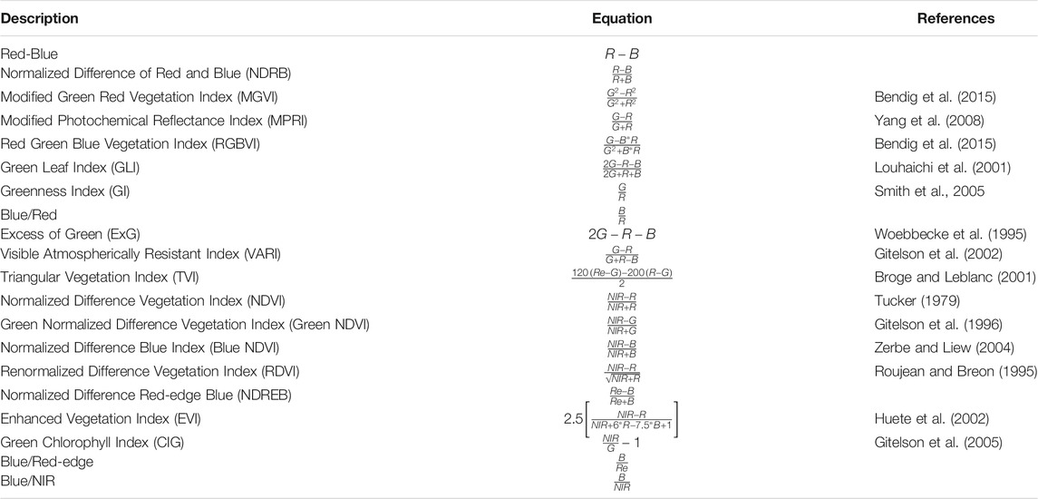
TABLE 1. Blue (B), green (G), red (R), red-edge (Re), and near infrared (NIR) band combinations for each of the vegetation indices tested for the separability analysis of kelp and water pixels.
Because JM and TD are only indicative of separability in cases of normality, the Shapiro-Wilk Normality test was used to determine whether the kelp and water pixel samples were normally distributed after each index was applied. The Shapiro-Wilk Normality test is most reliable with small sample sizes, and accordingly, ten iterations of the Shapiro-Wilk Normality test were computed, each extracting 100 random samples from the 500 kelp samples and 500 water samples from each image acquisition and spectral index (Huang et al., 2016).
In order to identify kelp using a vegetation index, a threshold was identified, and pixels above this threshold were considered kelp canopy. Ideally, a single threshold would have been used for all images, but differing sensors, illumination conditions, and kelp condition necessitated a more dynamic approach. For each image, histograms were calculated from vegetation index values (Figure 4). For images containing both kelp and water, histograms displayed a bimodal signature, with one peak characterizing kelp pixels and the other characterizing water. The locations of the “kelp” peak and the “water” peak were identified using the function findpeaks in MATLAB (2018). The value of the vegetation index at the midpoint between these two peaks was calculated, and this vegetation index value was used as the unique, image-based classification threshold (Figure 4). If only one peak was identified (i.e., the image was dominated by either kelp or water pixels), the function gradient was applied in MATLAB (2018) to identify potential shoulders within the histogram. In these images, the vegetation index value at the midpoint between the shoulder and the peak was used as the unique, image-based classification threshold (Supplementary Figure S2).
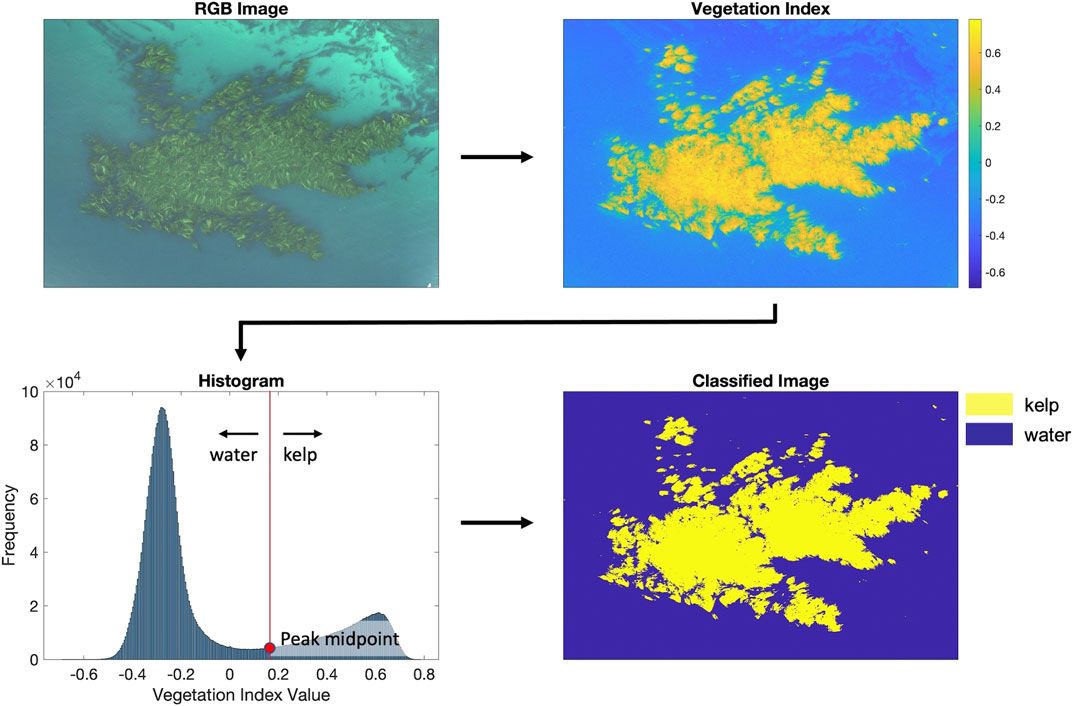
FIGURE 4. Methodology used in the detection of the presence or absence of kelp in each pixel. For each image, we applied the vegetation index (Red-Blue and NDREB) and calculated histograms to find unique thresholds for image classifications.
Using the separability measures, the best performing RGB-based index (Red-Blue, see results) and the best performing red-edge or NIR-based index (Normalized Difference Red-edge Blue (NDREB), see Results) were identified. An accuracy assessment was performed to compare the automated classifications from these two indices. Using the same 10 images used within the TD and JD separability analysis, 50 random points within each image were sampled for a total of 500 random points (211 kelp points, 289 water points). The points were manually determined to be either a kelp or water pixel, the number of pixels each index accurately classified was calculated.
NDREB yielded the highest accuracy, and the NDREB histogram-based automated classification was applied to each image in Honeymoon Cove tidal surveys, Arroyo Quemado tidal surveys, Arroyo Quemado current surveys, and Honeymoon Cove time series (Supplementary Figures S3–S6). The number of kelp pixels in each classified image was multiplied by the area of each pixel (10 cm × 10 cm) to calculate kelp canopy area for each image. For the tidal analysis, the identified kelp canopy area from Arroyo Quemado was compared to ADCP tidal measurements from the SBC LTER project, and the identified kelp area from Honeymoon Cove was compared to NOAA/NOS/CO-OPS 1 min tidal measurements. The station-measured tidal height at the midpoint of each flight was used for comparison. For the current analysis, the identified kelp area from Arroyo Quemado was compared to ADCP current measurements from the SBC LTER project taken within the kelp forest at 12.5 m (from the bottom). The ADCP-measured current speed at the midpoint of each flight was used for comparison.
Biweekly imagery at Honeymoon Cove was collected from June 2018 to August 2019 for a total of 25 images. All flights were conducted at mid-tide (∼1 m) to reduce the impact of tides on surface canopy measurements. Flights were not restricted due to time of day or cloud coverage, however, flights were canceled if wind speeds exceeded 16 km/h or if there was any precipitation.
For qualitative comparisons between seasonal variations in kelp canopy area and environmental variables, SST measurements were collected from the NOAA National Data Buoy Center Station 9410660 and the measurements were aggregated to daily means. Additionally, maximum wave height data were collected from the Coastal Data Information Program’s (CDIP) nowcast alongshore wave-propagation model (O’Reilly et al., 2016). The model uses various parameters from sites located at 100 m intervals along the backbeach to calculate hourly estimates of maximum wave height at a depth of 10 m along the California coastline. Five sites that incorporated calculations from the backbeach within Honeymoon Cove (sites L0389–L0394) were selected and averaged by date and time. The daily maximum wave height was calculated for analysis.
Tidal height and current speed can be strongly correlated, and as a result, several statistical analyses were performed to detect and separate the effects of tides and currents on variations in kelp canopy area (Britton-Simmons et al., 2008). For each tidal survey (both Honeymoon Cove surveys and the Arroyo Quemado survey), a simple linear regression was applied to determine whether tidal height (independent variable) was significantly correlated with kelp canopy area (dependent variable). To test for potential differences between the Honeymoon Cove tidal surveys due to current speed, a one-way analysis of covariance (ANCOVA) was used to determine whether the Honeymoon Cove simple linear regression slopes from the two tidal survey dates were equal. To test for potential differences in the relationship between tidal height and kelp canopy area at Honeymoon Cove and Arroyo Quemado, an ANCOVA was used to determine if the simple linear regression slopes between the two sites were significantly different from each other.
For the Arroyo Quemado tidal and current surveys, multiple linear regression was used to determine whether tidal height and current speed (independent variables) were significantly correlated with kelp area (dependent variable; Britton-Simmons et al., 2008). Additionally, partial correlation coefficients were calculated to partition the variance in canopy area explained by tidal height or current speed (Britton-Simmons et al., 2008). Partial correlation coefficients measure the correlation between two variables while holding a specified covariate constant (i.e., correlation between tidal height and kelp canopy area while holding current speed constant, and the correlation between current speed and kelp canopy area while holding tidal height constant; Sokal and Rohlf, 1981). These additional analyses were performed to help distinguish the effect of tides and currents on kelp canopy area during the tidal and current surveys. Current data were only available at the Arroyo Quemado kelp forest (current data were not available during the Honeymoon Cove tidal surveys), and as a result, the multiple linear regression analysis and partial correlation coefficients were only calculated at this site.
The twenty vegetation indices yielded variable performances in the parametric separability analysis of kelp and water pixel samples (Figure 5). p-values from the Shapiro-Wilk Normality test, which indicate whether the data come from a normally distributed population, varied within and between the ten iterations performed on each vegetation index. All of the data were not considered to be normally distributed (with p-values ranging from <0.001 to 0.35 for kelp and from <0.001 to 0.46 for water), which may introduce bias into the JM and TD tests. However, these results were only used to help inform the optimal vegetation index for analysis. For the RGB-based vegetation indices, Red-Blue exhibited the highest cumulative JM and TD values (1.29 and 1.47, respectively), while Blue/Red exhibited the next highest cumulative values (1.29 and 1.42, respectively; Figure 6). None of the RGB-based vegetation indices yielded completely separable results. For vegetation indices that included either the red-edge or NIR band, each index exceeded separability scores of 1.5 or greater for both JM and TD. NDREB exhibited the highest cumulative JM and TD values (1.99 and 1.99, respectively), while Blue/Red-edge exhibited the next highest cumulative values (1.96 and 1.99, respectively; Figure 7).
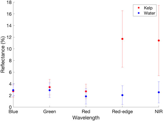
FIGURE 5. Mean and standard deviation for the manually classified and digitized kelp and water pixels for from the blue, green, red, red-edge, and NIR bands. These values were used as inputs to the vegetation indices used in the parametric separability analysis.
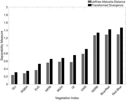
FIGURE 6. JM and TD values for the 10 RGB vegetation indices, with 0 being no separability between classes and 2 being complete separability.
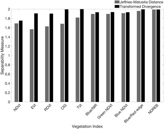
FIGURE 7. JM and TD values for the 10 red-edge or NIR-based vegetation indices, with 0 being no separability between classes and 2 being complete separability.
The Red-Blue and NDREB performances in separating kelp and water pixel samples led to further analysis of these vegetation indices for use in the histogram-based automated classification. Red-Blue exhibited an overall accuracy of 67% in identification of the randomly selected 500 pixels, with an accuracy of 76.3% for kelp and 60.2% for water. The index NDREB exhibited an overall accuracy of 93%, with an accuracy of 88.6% for kelp and 96.2% for water. Red-Blue consistently classified submerged fronds as floating canopy, as exemplified by the lower classification accuracy for water. Additionally, Red-Blue often classified visible substrate (i.e., on a day with high water clarity) as floating kelp canopy.
Both indices were sensitive to water surface features (ripples and waves), remnant glint artifacts, shadows (i.e., from steeply sloped shoreline), often mis-classifying these features as kelp. Darkly shaded kelp fronds and remnant glint on kelp fronds were often mis-classified as water. Overall, NDREB was more robust and was able to accurately classify kelp and water pixels across a wide variety of environmental conditions and was used to distinguish kelp from water in all further analyses.
A simple linear regression showed tidal height was significantly correlated with kelp canopy area in both Honeymoon Cove tidal surveys (F (1,5) = 213.19, p < 0.001 and F (1,4) = 10.39, p = 0.03, respectively) and in the Arroyo Quemado tidal survey (F (1,5) = 134.69, p < 0.001; Figure 8). Tides had a large impact on the amount of kelp canopy exposed in southern California aerial imagery, as a 1 m increase in tidal height resulted in a 30.26% and 32.30% decrease in kelp canopy area during the first and second Honeymoon Cove tidal surveys, respectively, and a 15.67% decrease in kelp canopy area at the Arroyo Quemado kelp forest (Figure 8).
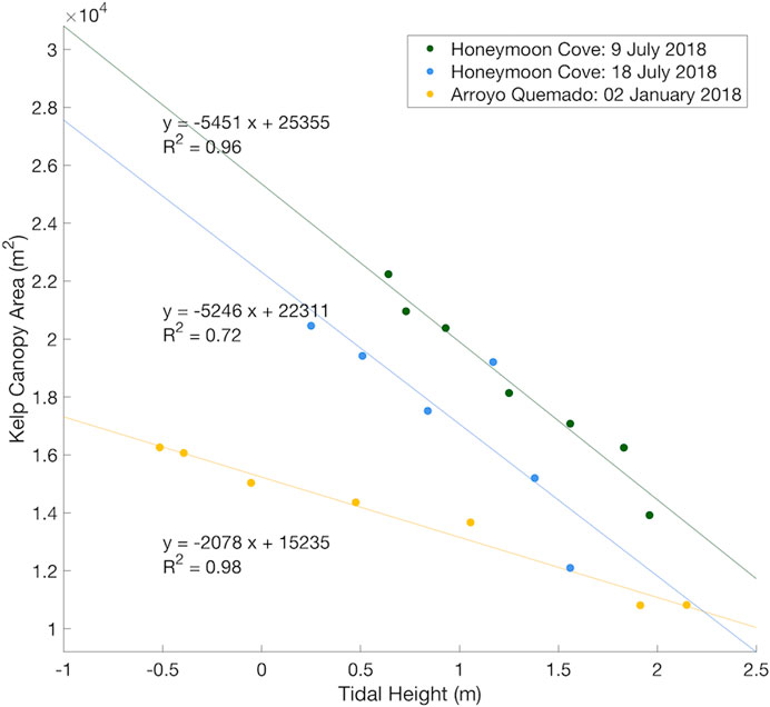
FIGURE 8. Regression analysis between kelp canopy area and tidal height for each tidal survey completed at Honeymoon Cove (n = 7, n = 6) and Arroyo Quemado (n = 7).
The reduction in canopy area with increasing tidal height was similar between the two Honeymoon Cove tidal surveys, as the slopes of the Honeymoon Cove regression lines (one for each tidal survey date) were not significantly different (F (1,9) = 0.02, p = 0.90). The reduction in canopy area with increasing tidal height was greater in both Honeymoon Cove surveys than it was at Arroyo Quemado (F (1,10) = 60.18, p < 0.001 and F (1,9) = 6.83, p = 0.02, respectively).
During the Arroyo Quemado tidal survey, current speeds generally increased as tidal heights reached their minimum (Figure 9). During this survey, tidal height was significantly correlated with current speed (F (1,5) = 23.6, p = 0.005). However, the relationship between tidal height and current speed was variable at the Santa Barbara site, and over the course of the two weeks following the tidal height survey, tides and currents were not correlated (R2 = 0.0009). The multiple regression analysis from the Arroyo Quemado tidal survey showed a significant negative relationship between tidal height and kelp area (p = 0.01; Table 2). The relationship between current speed and kelp area was positive but insignificant (p = 0.65; Table 2). The partial correlation analysis showed that when the effects of current speed were controlled, tidal height explained 86.90% of the observed variation in and kelp canopy area. By contrast, contribution of current velocity explained only 5.7% of the observed variation in canopy area, and this result was not significant (p = 0.65; Table 2).
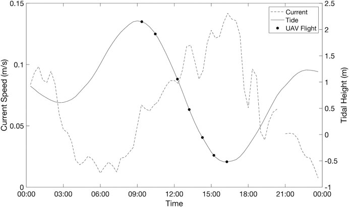
FIGURE 9. Temporal variations in tidal height and current speed during each flight of the single-day Arroyo Quemado tidal survey.

TABLE 2. Multiple regression and partial correlation analysis results from the Arroyo Quemado tidal survey.
Current speeds ranged from 0.02 to 0.13 m/s across the five dates, which was representative of average conditions in the Arroyo Quemado kelp forest during 2019 as a whole (Figure 10; annual average of 0.085 ± 0.066 m/s). Current speed exhibited a negative linear relationship with kelp canopy area, with canopy area declining by 31.99% for a 0.1 m/s increase in current velocity (F (1,5) = 6.05, p = 0.09; Figure 11). While this relationship was not highly significant, the magnitude of the current effect was relatively large.
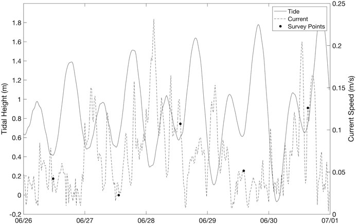
FIGURE 10. Temporal variations in tidal height and current speed during each flight of the multi-day Arroyo Quemado current surveys.
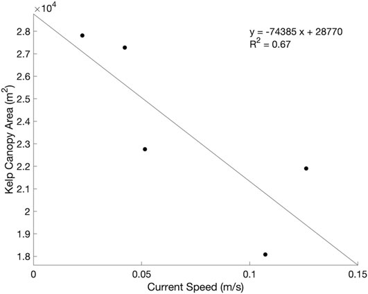
FIGURE 11. Regression analysis between kelp canopy area and current speed during the Arroyo Quemado current surveys.
During these five dates, there was no consistent relationship between tidal height and current speed (Figure 10) and the two were not significantly correlated (F (1,5) = 1.92, p = 0.23). The multiple regression analysis from the Arroyo Quemado current survey showed neither a significant effect of current speed on kelp area, nor a significant effect of tidal height (F (2,5) = 2.01, p = 0.33). The partial correlation analysis showed that variability in current speed accounted for a large amount of variability in kelp area during the current survey, this relationship was not statistically significant (p = 0.26), likely due to the limited number of data points (n = 5).
The mean kelp canopy area in Honeymoon Cove from June 2018 to August 2019 was 6,763.2 m2, but there was a high amount of variability about this mean. With a standard deviation of 7,104.6 m2, the coefficient of variation across the 25 surveys was 105%. Changes in kelp canopy area occurred over a seasonal cycle with kelp area maximums in mid-summer and minimums in winter (Figure 12). There was also pronounced seasonal variability, as patch level declines and increases in kelp canopy each progressed for about four months (from late summer to fall and from spring to early summer, respectively) before reaching maximum or minimum values (Figure 12). These gradual changes coincided with SST patterns, with kelp area declining to 3.14% of the overall time series mean area in mid-September after mean SST increased during the summer months (20.34 ± 1.20°C). Kelp canopy recovered to 104.48% of the mean kelp canopy area in June after mean SST decreases in the winter (15.64 ± 0.61°C; Figure 12) persisted through May. Rapid changes also occurred within seasonal time spans, as evidenced by kelp recovery from late October to late November (212.15 m2–8,990.92 m2) once the mean SST began to cool during the fall months (19.24 ± 0.36°C), followed by a rapid decline in kelp area to 169.87 m2 that corresponded to large wave events that began in late November (maximum wave height of 2.87 m). Kelp canopy area persisted below 10% of the mean kelp canopy area until April, when wave events began to subside and SST remained low (Figure 12).
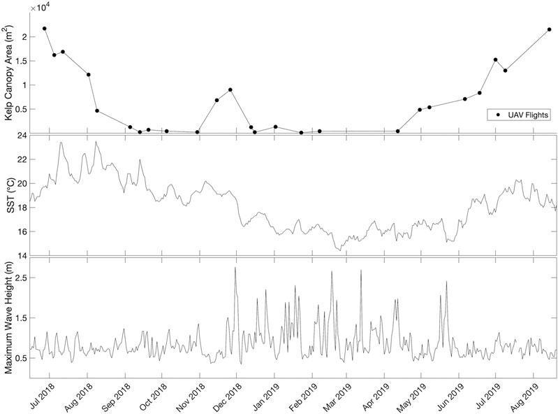
FIGURE 12. Honeymoon Cove UAV-derived time series of kelp canopy area from June 2018 to August 2019.
Our results demonstrate strong potential for using UAVs for repeat monitoring of floating kelp canopy on local scales. Flights were conducted for our area of interest using one battery set (20–30 min flights), allowing for relatively quick data collection. Additionally, mostly automated processing workflows (reflectance corrections, photogrammetry workflow, and classifications) allowed for dataset manageability, as processing took about 5 h from start to finish (about 4.5 h were automated). This time would decrease with more computing power and/or GPU processing.
Our automated method for detecting kelp canopy can be applied to both multispectral and RGB UAV imagery and is accurate across a range of weather, ocean, and illumination conditions. This robustness is important as there are a number of challenges associated with UAV-based remote sensing in coastal zones (Hodgson et al., 2013; Bevan et al., 2016; Schaub et al., 2018). Weather conditions, including precipitation and high wind, are common limiting factors in UAV deployment. Sun can also be a limiting factor for marine applications, as glint features on the water surface are challenging for photogrammetric software packages to manage. During stitching, the software may use glint artifacts as tie points to stitch two non-neighboring images in error, or it may be unable to find tie points altogether due to the lack of viable pixels. Additionally, any remaining glint in orthomosaics can introduce spectral noise and bias classification efforts. Sun glint can be reduced or avoided by collecting data on overcast days or by flying when the sun is at lower angles in the sky, but this is not always possible as flights may need to be conducted at a certain tidal stage. By introducing sun glint masks into our image processing workflow, photogrammetry alignment success increased in almost every flight and the presence of sun glint greatly decreased in final orthomosaics.
Another challenge of using UAV imagery for analysis in marine ecosystems includes changing illumination conditions within flights (i.e., on a partly cloudy day when the sun continuously emerges and disappears behind clouds) and between flights (i.e., flying on an overcast day and flying on a sunny day). Despite spectral corrections with reflectance panels, these variations impact output reflectance values and cause spectral inconsistencies. As a result, using supervised classification schemes to distinguish kelp from water is difficult, as the training data often do not adequately cover the spectral ranges observed through each flight (Taddia and Russo 2019). Additionally, while vegetation indices help to distinguish kelp from water, the threshold for separation strongly depends on image-specific spectral values, in turn necessitating image-specific thresholds (Taddia and Russo 2019). Our dynamic thresholding procedure removed the subjectivity and visual bias involved with manual threshold selection and produced a classification that was highly accurate in classifying both kelp and water.
Our highest accuracies were achieved using multispectral imagery, and a number of other studies have demonstrated the utility of multispectral imagery in detecting kelp canopy (Jensen et al., 1980; Cavanaugh et al., 2010). While many traditional floating algae indices depend on the NIR band (Tucker 1979; Hu 2009; Cavanaugh et al., 2010; Xing and Hu 2016), the NDREB index, our highest preforming index, takes advantage of the high red-edge and low blue reflectance of kelp, as compared to the higher blue and lower red-edge reflectance of water, resulting in a stronger separation potential than traditional NDVI. Giant kelp is a brown alga, and spectrally differs from both green vegetation and green algae, as it lacks the chlorophyll b pigment. There is high reflectance between the absorption peaks of chlorophyll a and chlorophyll c (the orange-edge; Bell et al., 2015b; Schroeder et al., 2019b). Combined with the high reflectance of seawater in the blue portion of the visible spectrum, there is a larger difference between the blue and red-edge/NIR than there is between the red and red-edge/NIR.
Additionally, accuracies of >60% could be achieved using RGB imagery using a simple subtraction between the red and the blue band. This indicates potential for kelp mapping using accessible low-cost UAV platforms that come with digital cameras. However, users should be aware that RGB imagery is more sensitive to the misclassification of submerged kelp fronds and visible substrate (i.e., on a day with high water clarity).
Floating kelp canopy appears similar to submerged canopy in the visible range of the spectrum, yet the magnitude of NIR reflectance is much greater for floating canopy than for submerged canopy (Schroeder et al., 2019a, Schroeder et al., 2019b). As a result, RGB-based indices may have a hard time distinguishing between floating and submerged canopy when submerged canopy is visible. However, this could be a benefit for certain applications, as it indicates potential for mapping of submerged fronds using RGB imagery. While we lose submerged canopy data in the NIR, the variability in water clarity, environmental conditions, and the amount of floating canopy result in an inconsistent ability to detect submerged canopy–even when the NIR is excluded during detection efforts. Using the NIR reduces the error associated with this variability and allows us to isolate floating canopy.
While both indices misclassified surface features (ripples and waves), remnant glint artifacts, and shadows (i.e., from steeply sloped shoreline) as kelp, Red-Blue was much more prone to these errors. The difference in magnitude between kelp pixels and water pixels in the red-edge and the blue band is much larger than the difference in magnitude between kelp pixels and water pixels in the red and blue band (Figure 5). As a result, using the histogram approach, problematic features are more easily distinguishable from kelp with red-edge or NIR-based indices, as the signature of kelp is very strong in these histograms despite the added noise. With RGB-based indices, the kelp signal in Red-Blue is often small and can be masked by the noise.
The amount of kelp canopy mapped on the water surface at both Honeymoon Cove and Arroyo Quemado declined significantly with tidal height, suggesting that tides can bias aerial-derived metrics of kelp canopy. The effect of tide was not consistent between the two sites and was almost twice as strong at Honeymoon Cove, which may be the result of differing bed structures between the two sites. The Arroyo Quemado kelp forest is comprised of large discrete, offshore stands, while the Honeymoon Cove kelp forest is comprised of both large, dense kelp stands as well as small, sparse stands. At Arroyo Quemado, the depth linearly slopes downward from the shoreline (from about −1.5 m to −16.5 m), but the extensive rocky reef along the gradient allows for a continuous, dense canopy. Increases in tidal height submerged the edges of the canopy but did not submerge any central canopy features. At Honeymoon Cove, the depth slopes downward from the outer edges of the cove to the center (from about 0 m to −8 m). There is extensive and continuous rocky reef along the shallow edges of the cove, but the reef in the center is much more fragmented. As a result, dense aggregates of kelp grow along edges, and these behave similarly to the beds at Arroyo Quemado as tidal height increases. However, the patchy, fragmented aggregates in the center of the cove often only consist of a few individuals, and these become fully submerged as the tide increases (Figure 1). Kelp forest demographics might also influence the impacts of tides by controlling the fraction of canopy vs. subsurface fronds.
A region’s tidal range will clearly influence the degree to which UAV estimates of canopy area are affected by tides. Southern California has a generally low tidal range (∼2 m) compared to some other global regions (i.e., Southeast Alaska, ∼9 m). Yet, even this small range impacted kelp canopy coverage by over 15% at Arroyo Quemado and over 30% at Honeymoon Cove. This result disagrees with previous work that estimated the weak tidal fluctuations in Santa Barbara had no effect on kelp canopy coverage estimates from Landsat satellite imagery (Cavanaugh et al., 2010, 2011). However, the higher resolution of the UAV imagery and experimental design aimed at isolating the effects of tides likely enabled us to more clearly detect the tidal effect. Bell et al. (2020) also used Landsat imagery for kelp canopy detection and found inconsistencies in kelp biomass estimates between Landsat TM and ETM + sensors, which was attributed to the 8 day repeat difference between the satellites imaging at different points in the tidal cycle. Aggregating Landsat biomass estimates (30 m resolution) to a seasonal scale (3 months) was sufficient for correcting for tidal effects (Bell et al., 2020).
Tidal height explained 87% of the variation in kelp canopy area during the Arroyo Quemado tidal survey, which is consistent with findings from other regions with similar tidal signals, such as San Juan Island, WA (Britton-Simmons et al., 2008). Kelp beds adjacent to San Juan Island experience tidal ranges of 2–3 m and are mainly comprised of bull kelp (Nereocystis luetkeana). Britton-Simmons et al. (2008) found that tidal height explained between 67% and 95% of observed variability in kelp area across six different sites near San Juan Island, which included differing kelp densities, bathymetry, coastline shapes, and current strength. While both giant kelp and bull kelp form floating canopies, they exhibit unique morphological features. Each giant kelp blade is attached to a pneumatocyst that buoys it to the surface (Graham et al., 2007), while bull kelp blades for one individual grow from a single, large (15 cm diameter) pneumatocyst (Amsler and Neushul, 1989; Schroeder et al., 2019a). As a result, giant kelp canopies consist of stipes, pneumatocysts, and blades, while bull kelp canopies mainly consist of stipes and pneumatocysts; bull kelp fronds often remain submerged (Schroeder et al., 2019a). While these morphological differences responded similarly to tidal fluctuations in southern California and San Juan Island, they may exhibit different effects in regions with more extreme tidal fluctuations. Additionally, currents and tides are often related, and these factors have the ability to interact and impact the amount of canopy visible to the sensor. Currents and tides were significantly correlated during the Arroyo Quemado tidal survey, and while multiple regression and partial correlation coefficients show that variations in kelp canopy were likely due to tidal fluctuations, it remains difficult to concretely separate the effect of either tides or currents on floating canopy area.
Canopy area was not significantly correlated (at the p = 0.05 level) with current speed during the tidal surveys or in the surveys conducted across multiple days at similar tidal stages. However, the relationship may have been significant if more samples were included in the study. While the p-value for this relationship was above 0.05 (p = 0.09), the effect size was large, as a 0.1 m/s increase in current speed reduced the amount of floating canopy by over 31%. More data is needed to determine whether there is in fact a relationship between these relatively low current speeds and visible canopy area. In their study of bull kelp along San Juan Island, Britton-Simmons et al. (2008) found that for a bed where current speeds never exceeded 0.4 m/s, there was no significant relationship between current speed and the amount of visible kelp on the water surface (Britton-Simmons et al., 2008). In contrast, the effects of current speed on the canopy areas of the other five kelp beds from Britton-Simmons et al., 2008 were found to be highly significant, but current speeds ranged much higher at these sites (>1 m/s). While low current speeds may impact giant kelp and bull kelp similarly, the relationship may change as current speed increases. Bull kelp blades begin to stream laterally with moderate amounts of current, resulting in larger floating canopies. As a result, the relationship between the percentage of bull kelp bed visible and current speed is often non-linear and difficult to quantify, as it varies with geographic shading, coastline shape, and bathymetry (Britton-Simmons et al., 2008). The spatial variation in current dynamics around kelp beds is extremely dynamic, and necessitates site-specific corrections–especially in places with high current ranges (Britton-Simmons et al., 2008).
Our UAV time series dataset represents a high-resolution assessment of high-frequency variability in kelp canopy area. Previous studies have demonstrated the effectiveness of deriving time series of kelp canopy biomass or area from aerial and satellite imagery, but many of these analyze data on quarterly or annual time scales, which limits the potential for characterizing seasonal dynamics (Jensen et al., 1980; Deysher 1993; Berry et al., 2005; Stekoll et al., 2007; Cavanaugh et al., 2010; Cavanaugh et al., 2011; Cavanaugh et al., 2019; Bell et al., 2015b; Bell et al., 2020; Pfister et al., 2018; Rogers-Bsennett and Catton 2019; Schroeder et al., 2019a). This UAV dataset provides a novel view into the feasibility for collecting long-term datasets at high spatial and temporal resolution, and the potential for understanding the rapid, sub-seasonal variations in canopy dynamics.
The Honeymoon Cove time series displayed a high degree of intra-annual variability in giant kelp abundance. Previous studies in southern and central California have found that kelp canopies and standing crop in wave exposed locations typically exhibit a seasonal cycle with maximums in the late summer to early fall and minimums in late winter to early spring (Graham et al., 1997; Reed et al., 2008; Cavanaugh et al., 2011). This pattern has been attributed to wave disturbance in the winter followed by recovery during the spring and summer. However, nutrient availability can be low in southern California during summer months, which can lead to reduced growth rates and canopy dieback (Clendenning and Sargent, 1971; Zimmerman and Kremer, 1986). Our time series of canopy showed evidence of both of these processes superimposed on one another. Increased temperature and decreased nutrients in the late summer were associated with gradual declines in kelp coverage. However, water temperatures decreased in the fall before the onset of major wave disturbance, and this was associated with a short-lived increase in kelp cover (Figure 12). This increase may have been linked to increased nutrient levels, however, a number of other factors may have been involved, including increased light availability and an increase in unoccupied substrate following the late fall kelp decline. The first large wave event of the winter yielded immediate kelp declines, and abundance remained low until wave events began to subside in the spring. As temperature and nutrient conditions became more favorable, kelp abundance continued to increase until reaching a peak in late summer.
One of the benefits of UAV-based monitoring is the flexibility in timing of data collection. For example, repeated UAV surveys provide one way for characterizing variability in the phenology of giant kelp abundance across sites and years. The timing of kelp growth and dieback is likely to be important as it might influence cycles of reproduction and growth of species that depend on kelp for food, e.g., sea urchins. UAV surveys can also be used to document the effect of discrete disturbances such as large wave events or marine heatwaves. Logistically, UAVs allow the operator to mitigate the impacts of environmental conditions such as clouds, tides, and wind on data quality. Cloud cover limits satellite acquisitions while UAVs can be flown below clouds or surveys can be planned for clear days. Here we have shown the potential impacts of tides on canopy area estimates and the difficulty of applying a universal correction factor across different sites. UAV surveys can be planned around tidal cycles to reduce the need to correct for tides.
The spatial and temporal capabilities of UAV imagery make these platforms useful for local mapping of giant kelp canopies at high spatial resolution, but the potential effects of tides and current should be considered when planning UAV surveys. Collecting repeated measurements of kelp canopy area at a relatively small spatial scale (e.g., less than a few m2) is challenging, as diving efforts require extensive data collection, and estimates from most satellite platforms do not provide suitable resolutions (Britton-Simmons et al., 2008; Reed et al., 2008, Reed et al., 2009; Schroeder et al., 2019a). UAVs provide the ability to collect data over larger areas than would be possible with other in situ methods and provide much higher resolution than most satellite datasets. In addition, they are typically much more cost effective than occupied aerial surveys. Therefore, UAVs can be used to map kelp in small, sparse beds close to the coast, to create high spatial resolution time series, and to examine the impacts of discrete events such as large wave events. This high spatial resolution comes at the expense of the broad spatial coverage of satellites, and neither method can fully replace the other. Ultimately, the choice of which method to use is highly dependent on the ecological questions being asked.
The raw data supporting the conclusions of this article will be made available by the authors, without undue reservation. A conservation institution has used the glint masking methods developed in this study to produce an open-access tool for glint removal of aerial imagery (https://doi.org/10.21966/3cpa-2e10).
KaC, KyC, and TB conceived the study. KaC, KyC, TB, and EH performed UAV flight planning and conducted UAV flights. KaC and EGH processed the data. KaC led algorithm development. KaC and KyC led the analysis and wrote the manuscript. All authors contributed to results interpretation and manuscript draft revisions.
Funding was provided by the U.S. Department of Energy ARPA-E (grant number DE-AR0000922), the U.S. National Science Foundation which provided funding for the SBC LTER (grant number OCE 1831937), and the Nature Conservancy (grant number 02042019-5719).
The authors declare that the research was conducted in the absence of any commercial or financial relationships that could be construed as a potential conflict of interest.
The Supplementary Material for this article can be found online at: https://www.frontiersin.org/articles/10.3389/fenvs.2020.587354/full#supplementary-material.
The content of this manuscript has been published as part of the thesis of KaC. We would like to thank the field and laboratory technicians who helped in the collection and processing of the UAV data.
Amsler, C. D., and Neushul, M. (1989). Diel periodicity of spore release from the kelp Nereocystis luetkeana. J. Exp. Mar. Biol. Ecol. 134, 117–127.
Bell, T. W., Allen, J. G., Cavanaugh, K. C., and Siegel, D. A. (2020). Three decades of variability in California’s giant kelp forests from the Landsat satellites. Remote Sens. Environ. 238, 110811. doi:10.1016/j.rse.2018.06.039
Bell, T. W., Cavanaugh, K. C., Reed, D. C., and Siegel, D. A. (2015a). Geographical variability in the controls of giant kelp biomass dynamics. J. Biogeogr. 42, 2010–2021. doi:10.1111/jbi.12550
Bell, T. W., Cavanaugh, K. C., and Siegel, D. A. (2015b). Remote monitoring of giant kelp biomass and physiological condition : an evaluation of the potential for the Hyperspectral Infrared Imager (HyspIRI) mission. Remote Sens. Environ. 167, 218–228. doi:10.1016/j.rse.2015.05.003
Bendig, J., Yu, K., Aasen, H., Bolten, A., Bennertz, S., Broscheit, J., et al. (2015). Combining UAV-based plant height from crop surface models, visible, and near infrared vegetation indices for biomass monitoring in barley. Int. J. Appl. Earth Obs. Geoinf. 39, 79–87. doi:10.1016/j.jag.2015.02.012
Berry, H. D., Mumford, T. F., and Dowty, P. (2005). Using historical data to estimate changes in floating kelp (nereocystis luetkeana and macrocystis integrifolia) in puget sound (Available at:http://depts.washington.edu/uwconf/2005psgb/2005proceedings/papers/F7_BERRY.pdf%0Apapers3://publication/uuid/A9C39740-8651-46F0-A52A-D1E89664AF5C.
Bevan, E., Wibbels, T., and Najera, B. M. Z. (2016). Using unmanned aerial vehicle (UAV) technology for locating, identifying, and monitoring courtship and mating behavior in the green turtle (Chelonia mydas) Techniques. Tech. 27 Herpetol. Rev. 47, 27–32.
Britton-Simmons, K., Eckman, J. E., and Duggins, D. O. (2008). Effect of tidal currents and tidal stage on estimates of bed size in the kelp Nereocystis luetkeana. Mar. Ecol. Prog. Ser. 355, 95–105. doi:10.3354/meps07209
Broge, N. H., and Leblanc, E. (2001). Comparing prediction power and stability of broadband and hyperspectral vegetation indices for estimation of green leaf area index and canopy chlorophyll density. Remote Sens. Environ. 76, 156–172. doi:10.1016/S0034-4257(00)00197-8
Castorani, M. C., Reed, D. C., Alberto, F., Bell, T. W., Simons, R. D., Cavanaugh, K. C., et al. (2015). Connectivity structures local population dynamics: a long-term empirical test in a large metapopulation system. Ecology. 96, 3141–3152. doi:10.1890/15-0283.1
Castorani, M. C., Reed, D. C., Raimondi, P. T., Alberto, F., Bell, T. W., Cavanaugh, K. C., et al. (2017). Fluctuations in population fecundity drive variation in demographic connectivity and metapopulation dynamics. Proc. Biol. Sci. 284. doi:10.1098/rspb.2016.2086
Cavanaugh, K. C., Kendall, B. E., Siegel, D. A., Reed, D. C., Alberto, F., and Assis, J. (2013). Synchrony in dynamics of giant kelp forests is driven by both local recruitment and regional environmental controls. Ecology. 94, 499–509. doi:10.1890/12-0268.1
Cavanaugh, K. C., Siegel, D. A., Raimondi, P. T., and Alberto, F. (2014). Patch definition in metapopulation analysis: a graph theory approach to solve the mega-patch problem. Ecology. 95, 316–328. doi:10.1890/13-0221.1
Cavanaugh, K. C., Reed, D. C., Bell, T. W., Castorani, M. C. N., Beas-luna, R., and Barrett, N. S. (2019). Spatial variability in the resistance and resilience of giant kelp in southern and baja California to a multiyear heatwave. Front. Mar. Sci. 6, 1–14. doi:10.3389/fmars.2019.00413
Cavanaugh, K. C., Siegel, D. A., Kinlan, B. P., and Reed, D. C. (2010). Scaling giant kelp field measurements to regional scales using satellite observations. Mar. Ecol. Prog. Ser. 403, 13–27. doi:10.3354/meps08467
Cavanaugh, K. C., Siegel, D. A., Reed, D. C., and Dennison, P. E. (2011). Environmental controls of giant-kelp biomass in the Santa Barbara channel, California. Mar. Ecol. Prog. Ser. 429, 1–17. doi:10.3354/meps09141
Changhui, Y., Yuan, Y., Minjing, M., and Menglu, Z. (2013). “Cloud detection method based on feature extraction in remote sensing images Int. Arch. Photogramm. Remote Sens. Spat. Inf. Sci. XL-2/W1,” in , 8th International Symposium on Spatial Data Quality, Hong Kong, China, May 30–June 1, 2013, 173–177.
Clendenning, K. A., and Sargent, M. C. (1971). Photosynthesis and general development in Macrocystis. Nova Hedwigia 32, 169–190.
Deysher, L. E. (1993). Evaluation of remote sensing techniques for monitoring giant kelp populations. Hydrobiologia. 260–261, 307–312. doi:10.1007/BF00049033
Dugan, J. E., Hubbard, D. M., Mccrary, M. D., and Pierson, M. O. (2003). The response of macrofauna communities and shorebirds to macrophyte wrack subsidies on exposed sandy beaches of southern California. Estuar. Coast. Shelf Sci. 58, 25–40. doi:10.1016/S0272-7714(03)00045-3
Gentry, R. R., Froehlich, H. E., Grimm, D., Kareiva, P., Parke, M., Rust, M., et al. (2017). Mapping the global potential for marine aquaculture. Nat. Ecol. Evol. 1, 1317–1324. doi:10.1038/s41559-017-0257-9
Gentry, R. R., Alleway, H. K., Bishop, M. J., Gillies, C. L., Waters, T., and Jones, R. (2019). Exploring the potential for marine aquaculture to contribute to ecosystem services. Rev. Aquacult., 499–512. doi:10.1111/raq.12328
Gitelson, A. A., Kaufman, Y. J., and Merzlyak, M. N. (1996). Use of a green channel in remote sensing of global vegetation from EOS- MODIS. Remote Sens. Environ. 58, 289–298. doi:10.1016/S0034-4257(96)00072-7
Gitelson, A. A., Kaufman, Y. J., Stark, R., and Rundquist, D. (2002). Novel algorithms for remote estimation of vegetation fraction, Remote Sens. Environ. 80 76–87. doi:10.1016/S0034-4257(01)00289-9
Gitelson, A. A., Viña, A., Ciganda, V., Rundquist, D. C., and Arkebauer, T. J. (2005). Remote estimation of canopy chlorophyll content in crops. Geophys. Res. Lett. 32, 1–4. doi:10.1029/2005GL022688
Graham, M. H., Harrold, C., Lisin, S., Light, K., Watanabe, J. M., and Foster, M. S. (1997). Population dynamics ofgiant kelp Macrocystis pyrifera along awave exposure gradient. Marine Ecol. Prog. Ser. 148, 269–279. doi:10.3354/meps148269
Graham, M. H., Vásquez, J. A., and Buschmann, A. H. (2007). Global ecology of the giant kelp Macrocystis : from ecotypes to ecosystems. Oceanogr. Mar. Biol. 45, 39–88. doi:10.1201/9781420050943.ch2
Hakala, T., Markelin, L., Id, E. H., Scott, B., Theocharous, T., Id, O. N., et al. (2018). Direct reflectance measurements from Drones : sensor absolute radiometric calibration and system tests for forest reflectance characterization. Sensors (Basel). 18 (5), 14–17. doi:10.3390/s18051417
Hamilton, S. L., Bell, T. W., Watson, J. R., Grorud-Colvert, K. A., and Menge, B. A. (2020). Remote sensing: generation of long-term kelp bed data sets for evaluation of impacts of climatic variation. Ecology., 1–13. doi:10.1002/ecy.3031
Haralick, R. M., Shanmugam, K., and Dinstein, I. (1973). Textural features for image classification. IEEE Trans. Syst. Man Cybern. SMC. 3, 610–621. doi:10.1109/TSMC.1973.4309314
Harley, C. D., Hughes, A. R., Hultgren, K. M., Miner, B. G., Sorte, C. J., Thornber, C. S., et al. (2006). The impacts of climate change in coastal marine systems. Ecol. Lett. 9, 228–241. doi:10.1111/j.1461-0248.2005.00871.x
Hodgson, A., Kelly, N., and Peel, D. (2013). Unmanned aerial vehicles (UAVs) for surveying Marine Fauna: a dugong case study. PLoS One. 8, e79556–15. doi:10.1371/journal.pone.0079556
Hu, C. (2009). A novel ocean color index to detect floating algae in the global oceans. Remote Sens. Environ. 113, 2118–2129. doi:10.1016/j.rse.2009.05.012
Huang, H., Roy, D. P., Boschetti, L., Zhang, H. K., Yan, L., Kumar, S. S., et al. (2016). Separability analysis of Sentinel-2A Multi-Spectral Instrument (MSI) data for burned area discrimination. Rem. Sens. 8 (10). doi:10.3390/rs8100873
Huang, X., Liu, X., and Zhang, L. (2014). A multichannel gray level Co-occurrence matrix for multi/hyperspectral image texture representation. Rem. Sens. 6 (9). 8424–8445. doi:10.3390/rs6098424
Huete, A., Didan, K., Miura, T., Rodriguez, E. P., Gao, X., and Ferreira, L. G. (2002). Overview of the radiometric and biophysical performance of the MODIS vegetation indices. Rem. Sens. 83, 195–213. doi:10.1080/0965156x.2013.836857
Jensen, J. R., Estes, J. E., and Tinney, L. (1980). Remote sensing techniques for kelp surveys. Photogramm. Eng. Rem. Sens. 46, 743–755.
Kellaris, A., Badia, I. M., Gil, A., Neto, A., and Amaral, R. (2019). Using low.–cost drones to monitor heterogeneous submerged seaweed habitats : a case study in the Azores. New Jercy, NJ: Wiley. doi:10.1002/aqc.3189
Louhaichi, M., Borman, M. M., and Johnson, D. E. (2001). Spatially located platform and aerial photography for documentation of grazing impacts on wheat. Geocarto Int. 16, 65–70. doi:10.1080/10106040108542184
Miller, R. J., Lafferty, K. D., Lamy, T., Kui, L., Rassweiler, A., Reed, D. C., et al. (2018). Giant kelp, Macrocystis pyrifera, increases faunal diversity through physical engineering. Proc. Biol. Sci. 285 (1874), 20172571 doi:10.1098/rspb.2017.2571
Mora-Soto, A., Palacios, M., Macaya, E. C., Gómez, I., Huovinen, P., Pérez-Matus, A., et al. (2020). A high-resolution global map of giant kelp (macrocystis pyrifera) forests and intertidal green. 1–20 12 (4), 2-20. doi:10.3390/rs12040694
Nijland, W., Reshitnyk, L., and Rubidge, E. (2019). Satellite remote sensing of canopy-forming kelp on a complex coastline: a novel procedure using the Landsat image archive. Remote Sens. Environ. 220, 41–50. doi:10.1016/j.rse.2018.10.032
O’Reilly, W. C., Olfe, C. B., Thomas, J., Seymour, R. J., and Guza, R. T. (2016). The California coastal wave monitoring and prediction system. Coast. Eng. 116, 118–132. doi:10.1016/j.coastaleng.2016.06.005
Pfister, C. A., Berry, H. D., and Mumford, T. (2018). The dynamics of kelp forests in the northeast pacific ocean and the relationship with environmental drivers. J. Ecol. 106, 1520–1533. doi:10.1111/1365-2745.12908
Reed, D., Rassweiler, A., and Arkema, K. (2009). Density derived estimates of standing crop and net primary production in the giant kelp. Mar. Biol. 156, 2077–2083. doi:10.1007/s00227-009-1238-6
Reed, D. C., Rassweiler, A., and Arkema, K. K. (2008). Biomass rather than growth rate determines variation in net primary production by giant kelp. Ecology. 89, 2493–2505. doi:10.1890/07-1106.1
Rogers-Bennett, L., and Catton, C. A. (2019). Marine heat wave and multiple stressors tip bull kelp forest to sea urchin barrens. Sci. Repor. 9 (1). doi:10.1038/s41598-019-51114-y
Roujean, J. L., and Breon, F. M. (1995). Estimating PAR absorbed by vegetation from bidirectional reflectance measurements. Remote Sens. Environ. 51, 375–384. doi:10.1016/0034-4257(94)00114-3
Schaub, J., Hunt, B. P. V., Pakhomov, E. A., Holmes, K., Lu, Y., and Quayle, L. (2018). Using unmanned aerial vehicles (UAVs) to measure jellyfish aggregations. Mar. Ecol. Prog. Ser. 591, 29–36. doi:10.3354/meps12414
Schroeder, S. B., Boyer, L., Juanes, F., and Costa, M. (2019a). Spatial and temporal persistence of nearshore kelp beds on the west coast of British Columbia, Canada using satellite remote sensing. Remote Sens. Ecol. Conserv. 6, 327–343. doi:10.1002/rse2.142
Schroeder, S. B., Dupont, C., Boyer, L., Juanes, F., and Costa, M. (2019b). Passive remote sensing technology for mapping bull kelp (Nereocystis luetkeana ): a review of techniques and regional case study. Glob. Ecol. Conserv. 19, e00683. doi:10.1016/j.gecco.2019.e00683
Stekoll, M. S., Deysher, L. E., and Hess, M. (2006). A remote sensing approach to estimating harvestable kelp biomass. J. Appl. Phycol. 18, 323–334. doi:10.1007/s10811-006-9029-7
Stekoll, M. S., Deysher, L. E., and Hess, M. (2007). Eighteenth international seaweed symposium. Eighteenth Int. Seaweed Symp. doi:10.1007/978-1-4020-5670-3
Taddia, Y., and Russo, P. (2019). Multispectral UAV monitoring of submerged seaweed in shallow water.
Thomsen, M. S., Mondardini, L., Alestra, T., Gerrity, S., Tait, L., South, P. M., et al. (2019). Local extinction of bull kelp (durvillaea spp). Due to a Marine Heatwave. 6, 1–10. doi:10.3389/fmars.2019.00084
Tucker, C. J. (1979). Red and photographic infrared linear combinations for monitoring vegetation. Remote Sens. Environ. 8, 127–150. doi:10.1016/0034-4257(79)90013-0
Whitehead, K., Hugenholtz, C. H., Myshak, S., Brown, O., LeClair, A., Tamminga, A., et al. (2014). Remote sensing of the environment with small unmanned aircraft systems (UASs), part 2: scientific and commercial applications. J. Unmanned Veh. Syst. 02, 86–102. doi:10.1139/juvs-2014-0006
Whitehead, K., and Hugenholtz, C. H. (2014). Remote sensing of the environment with small unmanned aircraft systems (UASs), part 1: a review of progress and challenges. J. Unmanned Veh. Syst. 02, 69–85. doi:10.1139/juvs-2014-0006
Woebbecke, D. M., Meyer, G. E., Von Bargen, K., and Mortensen, D. A. (1995). Shape features for identifying young weeds using image analysis. Trans. Am. Soc. Agric. Eng. 38, 271–281. doi:10.13031/2013.27839
Xing, Q., and Hu, C. (2016). Mapping macroalgal blooms in the Yellow Sea and East China Sea using HJ-1 and Landsat data: application of a virtual baseline reflectance height technique. Remote Sens. Environ. 178, 113–126. doi:10.1016/j.rse.2016.02.065
Yang, Z., Willis, P., and Mueller, R. (2008). Impact of band-ratio enhanced awifs image to crop classification accuracy. Colorado, CO: Pecora Corporation.
Zerbe, L. M., and Liew, S. C. (2004). Reevaluating the traditional maximum NDVI compositing methodology: the normalized difference blue index. Int. Geosci. Remote Sens. Symp. 4, 2401–2404. doi:10.1109/igarss.2004.1369774
Zheng, G., Li, X., Member, S., Zhou, L., Yang, J., Ren, L., et al. (2018). Development of a gray-level Co-occurrence matrix-based texture orientation estimation method and its application in sea surface wind direction retrieval from SAR imagery. IEEE Trans. Geosci. Rem. Sens. 56, 5244–5260. doi:10.1109/TGRS.2018.2812778
Keywords: drones, kelp classification, kelp mapping, spatial variability, tidal height, current speed, ecological succession
Citation: Cavanaugh KC, Cavanaugh KC, Bell TW and Hockridge EG (2021) An Automated Method for Mapping Giant Kelp Canopy Dynamics from UAV. Front. Environ. Sci. 8:587354. doi: 10.3389/fenvs.2020.587354
Received: 25 July 2020; Accepted: 24 December 2020;
Published: 17 February 2021.
Edited by:
Sherry L. Palacios, California State University, Monterey Bay, United StatesReviewed by:
Maycira Costa, University of Victoria, CanadaCopyright © 2021 Cavanaugh, Cavanaugh, Bell and Hockridge. This is an open-access article distributed under the terms of the Creative Commons Attribution License (CC BY). The use, distribution or reproduction in other forums is permitted, provided the original author(s) and the copyright owner(s) are credited and that the original publication in this journal is cited, in accordance with accepted academic practice. No use, distribution or reproduction is permitted which does not comply with these terms.
*Correspondence: Katherine C. Cavanaugh, a2NjYXZhbmF1Z2hAZy51Y2xhLmVkdQ==
Disclaimer: All claims expressed in this article are solely those of the authors and do not necessarily represent those of their affiliated organizations, or those of the publisher, the editors and the reviewers. Any product that may be evaluated in this article or claim that may be made by its manufacturer is not guaranteed or endorsed by the publisher.
Research integrity at Frontiers

Learn more about the work of our research integrity team to safeguard the quality of each article we publish.