Assessing the Potential to Increase Landscape Complexity in Canadian Prairie Croplands: A Multi-Scale Analysis of Land Use Pattern

Increasing natural vegetation in agricultural landscapes can create habitat for beneficial organisms such as pollinators and the natural enemies of crop pests. Adding perennial vegetation can also support biodiversity conservation and climate change mitigation objectives. However, implementing such changes to agricultural land use across large geographic areas will require a strategic approach. This study examined the amount and distribution of uncultivated areas in Canadian prairie croplands, focusing on Alberta's agricultural zone (226,543 km²). The aim was to identify locations in this region that have potential for increasing non-crop land cover within fields. This assessment was based on a multi-scale model of landscape complexity that described the distribution of land cover as a function of the distance from field centers. It is based on the assumption that the land cover in the field neighborhood is an informative index of how much non-crop area might realistically be maintained or restored in the field itself; i.e., because neighboring lands will reflect the local environmental conditions that support the growth and establishment of non-crop vegetation as well as the likelihood that crop growers will remove areas from production. The model identified variation across the region in land cover distribution, with regions at latitudes between 52°N and 55°N demonstrating the greatest contrasts in the amount of non-crop land between the field and the field neighborhood scale. These findings suggest that there remains capacity for land use decision-makers to optimize the distribution of non-crop land covers in ways the reduce the differences between these scales (i.e., to increase non-crop covers within fields to better represent the neighborhood proportions). Modeling also revealed scale-dependent patterns, such as field margins without crops (400–500 m from field centers) broadly distributed across the region, and evidence that gradients in moisture and temperature have interacted with land use decisions to shape the proximity of non-crop area to fields.

Introduction

Increasing agricultural production to meet a growing global demand will require expansion and intensification of croplands (Godfray et al., 2010; Laurance et al., 2014; Egli et al., 2018), but this presents challenges for mitigating climate change and conserving biodiversity (Kleijn et al., 2009; Bustamante et al., 2014; Dalu et al., 2017; Karp et al., 2018). Ecological intensification of agriculture may offer a compromise by leveraging ecosystem services provided by organisms that boost yields while also minimizing impacts on natural systems (Bommarco et al., 2013).

One proposal is to promote non-crop vegetation within or near fields, which would reduce the simplification of agricultural landscapes caused by clearing and field expansion (Landis, 2017). Heterogeneity in non-crop land covers (hereafter landscape complexity), creates a greater number of off-field habitats providing opportunities for “spillover” into the crop (Birkhofer et al., 2018). The beneficial organisms that use these habitats may provide regulating services such as pest control and pollination to the surrounding crop. For example, complex agricultural landscapes have been associated with higher abundance and diversity of birds (Boesing et al., 2017), bats (Ancillotto et al., 2017), flower-visiting insects (Duarte et al., 2018) and the natural enemies of crop pests (Chaplin-Kramer et al., 2011), among other organisms.

There are further arguments for increasing landscape complexity. Restoring or augmenting semi-natural and other non-crop vegetation is an opportunity for carbon storage when trees, shrubs, and other perennial plants are permitted to grow (Smith, 2014; Lamb et al., 2016; Hungate et al., 2017; Williams et al., 2018). It may also support several other regulating ecosystem services through an increase in plant diversity (Asbjornsen et al., 2014), and conserve habitat for organisms that may not have direct benefits to agriculture (Phalan et al., 2011; Tscharntke et al., 2012).

However, meaningfully achieving these “win-win-wins” for agriculture, biodiversity and climate change mitigation will require that land use initiatives be implemented at broad geographic extents. Determining which parts of an agricultural region may be more or less amenable to improving landscape complexity can be used to target early efforts to those areas where there is greatest chance of success. For example, it may be easier to convince growers and land-owners to take land out of production in areas where there is already evidence of higher landscape complexity, but it is not uniformly distributed across all fields. In effect, the landscape context provides a measure of what improvements may be feasibly implemented.

This study examine landscape complexity in the Canadian Prairies. The region ranks among the world's largest contiguous agroecosystems, and has a cultivated footprint of more than 0.5 million km² (Agriculture and Agri-Food Canada, 2015). The focus is cropland in Alberta, which is distributed across most of the environmental and land use variability of these temperate grasslands (Ecological Stratification Working Group, 1995).

The primary aim is to identify which parts of this region have the highest potential for improving landscape complexity. That is, to identify where introducing additional non-crop land cover into fields and their surroundings may face the fewest challenges to implementation. For example, land conversion decisions may face resistance because natural vegetation is slow or costly to establish in certain regions, or because the land is highly-productive and value is placed on maximizing the area in production.

Finding such areas is done by building a spatial model of the distribution of non-crop land cover and how it varies with proximity to field centers. In this multi-scale approach, distributions of land cover at broad scales provide a target for the introduction of land cover within fields. Secondary aims of this study are to identify patterns in the distribution of these land covers, and how these may be associated with the broad environmental gradients that structure both vegetation and productivity.

Data and Methods

Study Area

The geographic focus is Alberta's agricultural zone, one of the most intensively cropped regions in the world (Foley et al., 2005), and an area that represents 30% of Canada's cropland and 20% of its annual farm income (Statistics Canada, 2016; Alberta Agriculture and Forestry, 2017). The dominant land cover is cropland, primarily in a 3-years cereal grain, oilseed, and pulse rotation. Forage lands are a secondary land cover vegetated in both introduced and native perennial grasses that are used for pasture and hay. Other semi-natural areas not in crop production are found both within and adjacent to fields, and they vary in frequency, size and type spatially along environmental gradients. These include patches of perennial grasses, shrubs, and deciduous trees. Planted tree shelterbelts, grass and forb road margins and wetlands of different classes, often surrounded in perennial vegetation, are also common throughout most of the study area (Doherty et al., 2018).

Land Cover

To characterize the variation in land cover across the region, a composite raster map was produced at 30 m resolution by combining data from several published sources in the order listed (Table 1). The product included a variety of land cover classes which were then simplified thematically to crop and non-crop areas. Non-crop areas also included paved and other human-modified areas such as roads, buildings, farm yards and in-field oil and gas well pads as these areas are likely to be surrounded in perennial vegetation and therefore contribute to landscape complexity (Forman, 2009). The binary thematic resolution of the land cover map was necessary given that better resolved and accurate products do not exist for this large extent. While this restricts inference about the types of vegetation that may contribute to landscape complexity, it is a simplification that may improve interpretation by reframing land cover as a land use decision (i.e., for crop production or otherwise).

TABLE 1

Table 1. Data layers used to produce a binary (crop/non-crop) land cover map for Alberta, Canada at 30 m spatial resolution.

Measuring Landscape Complexity

Landscape complexity was measured from the land cover map using randomly-selected field centers as sampling locations following an algorithmic approach implemented in R. Probable fields were identified using a nineteenth-century land survey which consistently divided the province of Alberta into 259 ha (1 mile by 1 mile) sections (Larmour, 2005). As a consequence of the gridding of the region, fields typically are nested within a section, with the quarter section (square subdivisions; 805 m by 805 m) describing the boundaries of most fields. The field centers (Figure 1) were randomly selected from all quarter section centroids with the conditions: (1) that the quarter must contain at least 50% crop cover (to ensure it at least partly represents a crop field); and (2) that the centers be no closer than 2.5 km apart (to improve statistical independence). These conditions were implemented using an algorithm that iteratively tested a randomly-permuted list of field centers for inclusion until no more could be added.

FIGURE 1

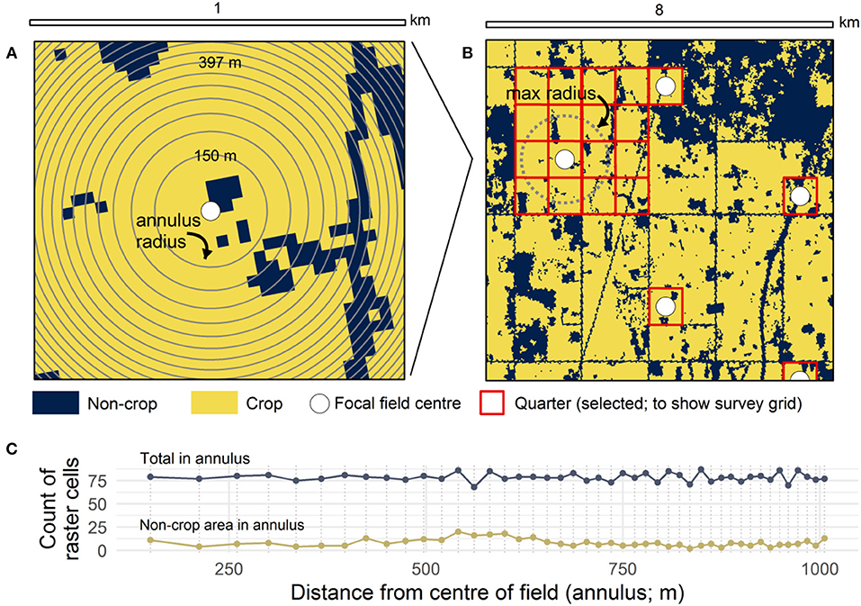
Figure 1. Illustration of the multi-scale method for measuring the proximity of non-crop land covers to field centers. (A) Forty-five annuli of decreasing radii, but approximately equal area, are measured from each field center; (B) Field centers are positioned at the center of quarter sections, the spatial unit that describes most fields in the region, and spaced a minimum of 2.5 km apart; (C) Counts of non-crop area raster cells and the total number of cells in each annulus in A used to find proportional cover. Non-crop raster cells are counted in the smallest annulus in which they fall.

Measuring landscape complexity requires assessing the variation in landscape structure. Metrics that have been used to describe landscape complexity are typically measured at a certain radius from a focal location, for example, by calculating the area of focal land covers, the proportional composition of crop, or the mean habitat patch size (e.g., Boesing et al., 2017). Because the distance from a field at which a non-crop land cover may have an effect is typically not known, this study uses an alternative approach that creates a multivariate index (or a “curve”) integrating the amount of land cover over multiple distances. This landscape complexity curve is determined by finding the proportion of non-crop area in 45 annuli of increasing radii (150–1,006 m) each of which is pre-determined to cover approximately the same total area to minimize sampling bias associated with smaller annuli (Figures 1A,C). Pixels from the rasterized land cover map were recorded in the annulus with the smallest radius in which they fell.

Landscape complexity, as defined here, is therefore a multi-scale metric for the proximity of non-crop land covers to the crop and more generally as an index of the variation in non-crop area both within and in the vicinity of a probable crop field. Annuli with the smallest radii describe conditions within the field itself (150–400 m; “within-field scale”), intermediate radii describe the field margins (400–500 m; “field-margin scale”) and larger radii which sample from multiple neighboring fields and semi-natural areas capture broader landscape variation (500–1,006 m; “neighborhood scale”). The neighborhood scale is intended to capture the local land cover conditions, and is applied in this study as an achievable upper target for restoring or augmenting non-crop land cover within the field itself. Because this scale samples neighboring fields it also measures how much of the landscape is in crop production.

Potential Environmental Drivers of Landscape Complexity

The study region encompasses several environmental gradients that influence both the dominant type of vegetation and primary productivity (e.g., temperature, moisture, latitude, and elevation; Ecological Stratification Working Group, 1995). These gradients also have the potential to affect the frequency of clearing and the rate of natural regrowth of vegetation, and may therefore interact with the behavior of land use decision-makers to shape the observed landscape complexity. Five covariates were chosen to test the importance of these environmental drivers (Figure 2). Mean annual temperature, total annual precipitation and plant available water in 120 cm of soil (April through August) were calculated as 9-years means (2009–2017) from an interpolated data product at the resolution of a survey township (36 sections; 93 km²; Alberta Agriculture and Forestry, 2018). Also included were agricultural limitations for crop production, a classification chiefly based on the workability of the soil by mechanized agricultural equipment (Agriculture and Agri-Food Canada, 2012), and ecoregions, a well-established categorical assessment of contiguous areas with consistent climate characteristics, similar vegetation, soil types, and elevation (Ecological Stratification Working Group, 1995).

FIGURE 2

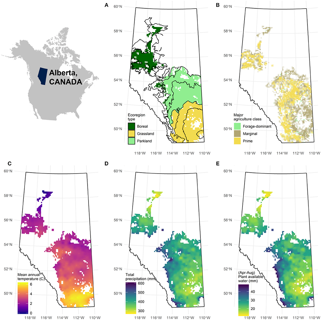
Figure 2. Environmental gradients in Alberta, Canada used as covariates when modeling landscape complexity. A colored pixel on the map represents a survey township containing agricultural land (N = 2,430). (A) Agricultural land intersects with 12 ecoregions (polygons) which can be broadly grouped according to their dominant non-crop vegetation; (B) Prime and marginal agricultural lands as determined by the limitations associated with cultivation; (C) Mean annual temperature (9 years means; 2009–2017); (D) Total precipitation (9 years means; 2009–2017); (E) Plant available water in the top 120 cm of soil found as a daily mean between April and August (9 years means; 2009–2017).

Modeling Landscape Complexity at Multiple Scales

Landscape complexity curves were modeled using a type of functional data analysis (FDA) known as function-on-scalar regression (Kokoszka and Reimherr, 2017; Wood, 2017). These models have functions (i.e., the landscape complexity curve) rather than the typical scalar values as response variables. A continuous function Y(x), was estimated from discrete data (e.g., Figure 1C, light line) using the proportion of non-crop area at each annulus radius, x. The model had the general form,

$\begin{array}{l}Y(x)=\mu (x)+{\alpha }_{p(i)}+{\alpha }_{p(i)}(x)+{\beta }_q(q,x)\\ +{\beta }_{r_1{r}_2}(r_1,r_2,x)+\dots +ϵ(x)\end{array}$

where μ(x) is the intercept function (i.e., the mean landscape complexity curve), α_p(i) and α_p(i)(x) represent the constant effect and functional effect, respectively, of level i of categorical variable p, β_q(q, x) reflects the functional effect of continuous variable q, β_r1r2(r₁, r₂, x) is the functional spatial effect given northing, r₁, and easting, r₂, and ϵ(x) is the residual function.

The model was fit using mgcv, a generalized additive modeling (GAM) package for R (Wood, 2017) using restricted maximum likelihood, by first setting up models with the refund package for R (Goldsmith et al., 2019) which provides optimized settings for FDA. The model assumed a Binomial data-generating process. Categorical constant effects were estimated parametrically, while categorical and continuous functional effects were estimated non-parametrically, with μ(x) and α_p(i)(x) functions entered as splines, and β_q(q, x) or β_r1r2(r₁, r₂, x) functions modeled as two- or three-dimensional tensor products, respectively. Spatial coordinates were projected and included in the model to account for spatial autocorrelation and to model geographic patterns not represented in other covariates. The maximum number of knots that could be used for estimating spline functional terms was set at 11 as a balance between overfitting and modeling abrupt changes in non-crop area over annulus distance. All covariates were scaled and centered.

Interpretation of the model involved examining the coefficient functions α_p(i)(x) and β_q(q, x) or generating predictions by excluding certain terms and systematically selecting input values to examine scenarios of interest. For example, predictions controlling for environmental covariates were generated by setting the relevant categorical functional or continuous functional terms to the zero function and entering categorical parametric coefficients as constants at the level with the most observations. Mapping was done by including the spatial term, β_r1r2(r₁, r₂, x), but not other environmental covariates, and generating predictions for the centroids of survey townships. The potential for increasing landscape complexity was assessed by finding the difference in the mean non-crop area prediction between neighborhood and within-field scales for the centroid of each survey township.

Results

The data set represented 14,527 randomly-selected quarter sections with a mean crop area of 79%, and a mean distance from nearest neighbor of 2,891 m. These quarter sections occupied 2,430 survey townships with a mean of 6 quarter sections in each (min = 1, max = 14), collectively sampling from an agricultural study region of 226,543 km². Forty-five annuli ranging from 150 m to 1,006 m in radius were assessed for each quarter (mean area per annulus = 7.1 ha). Data from the sampled quarters and their surroundings covered 6% of the total area under study.

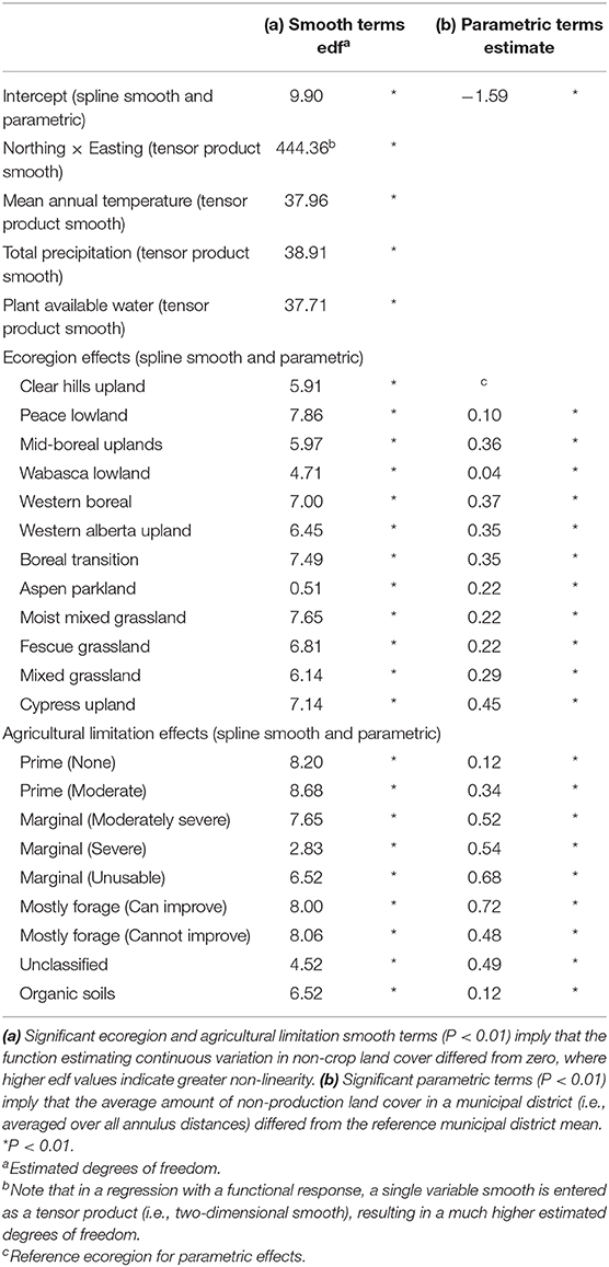
The model deviance explained was 32.2% ($R_{\text{adj}}^2$ = 0.355) with all constant parametric coefficients for categorical terms significantly different from zero (P < 0.01; Table 2a) suggesting the average proportion of non-crop area differed by ecoregion and agricultural limitation class. All functional non-parametric coefficient functions significantly differed from zero (P < 0.01; Table 2b) demonstrating a non-linear relationship between non-crop area and the distance from field centers, and that the included covariates mediate this relationship. The spatial term summarizing the effect of unmodelled geographic variables also had an effect on the landscape complexity curve (Northing × Easting; Table 2b).

TABLE 2

Table 2. Modeling of non-crop land cover variation.

The average trend in the proximity of non-crop area to field centers is that inside fields (150–400 m) there tend to be lower proportions of non-crop area than in the surrounding landscape (500–1,006 m; Figure 3). Thus, focal crop fields were not typically surrounded on all sides by other crop fields (a situation that would produce no difference between these two scales). However, there is spatial variation across the region in the proximity of non-crop areas to fields, after controlling for environmental covariates. This pattern is evident in the geographic differences in the predicted amount of non-crop cover at the within-field scale (e.g., Figure 4A), and at the neighborhood scale (e.g., Figures 4C,D). The field margin scale (400–500 m; e.g., Figure 4B) is more conserved across the province.

FIGURE 3

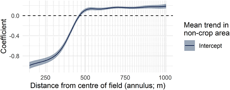
Figure 3. The model intercept function (or mean landscape complexity curve) shown with two standard errors. The curve represents the estimated effect on the proportion of non-crop area and how it varies over distance from the center of an average field. Vertical dotted lines in this and subsequent figures indicate annulus radii at which fields were measured, providing support for the model.

FIGURE 4

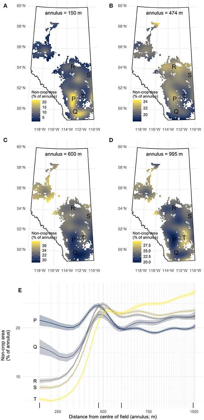
Figure 4. Predictions from the model while controlling for all covariates except the spatial term. Non-crop area is shown at four different annuli to demonstrate: (A) the field scale; (B) the field margin scale; (C,D) the neighborhood scale. (E) Landscape complexity curves at four locations (P, Q, R, S, and T) represent predictions across all scales and are intended to illustrate how the entire curve varies over the study region.

Most ecoregions (Figure 5) and agricultural limitation classes (Figure 6) had a characteristic landscape complexity curve, with these coefficient function plots demonstrating deviations in the coefficient from the mean landscape complexity curve (i.e., from Figure 1). All climatic variables also exerted effects on the shape of the landscape complexity curves (Figure 7). Trends for scales larger than the field margin scale (400–1,006 m) were generally similar for temperature and moisture-related variables. At the within-field scale, higher temperatures, and drier soils resulted in less non-crop area (mean annual temperature, plant available water; Figure 7).

FIGURE 5

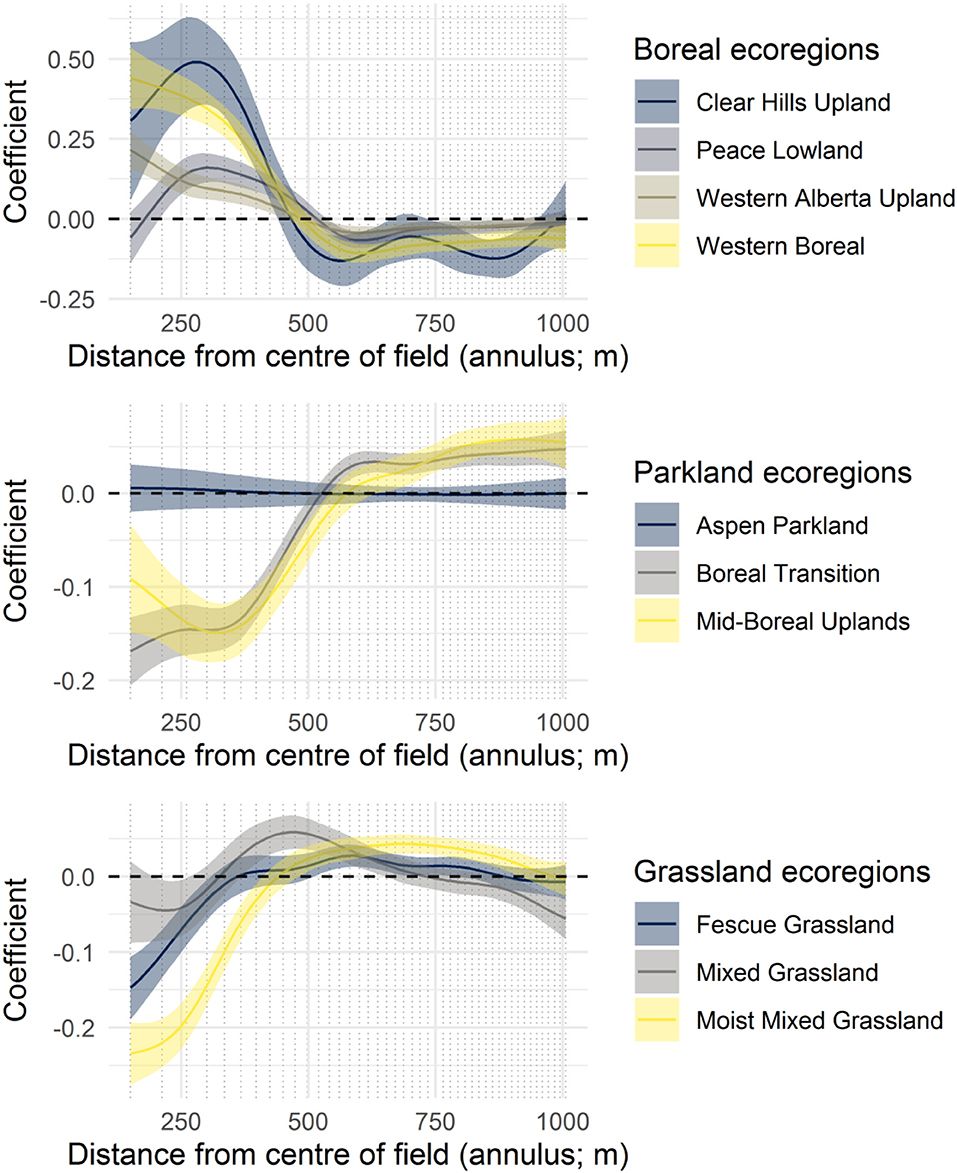
Figure 5. The coefficient functions for twelve ecoregions, grouped by their dominant non-crop vegetation. Curves demonstrate deviations from the mean landscape complexity curve (Figure 3).

FIGURE 6

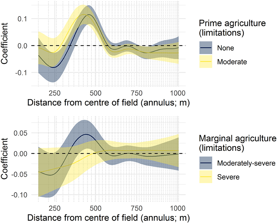
Figure 6. The coefficient functions for four agricultural limitation classes. Curves demonstrate deviations from the mean landscape complexity curve (Figure 3).

FIGURE 7

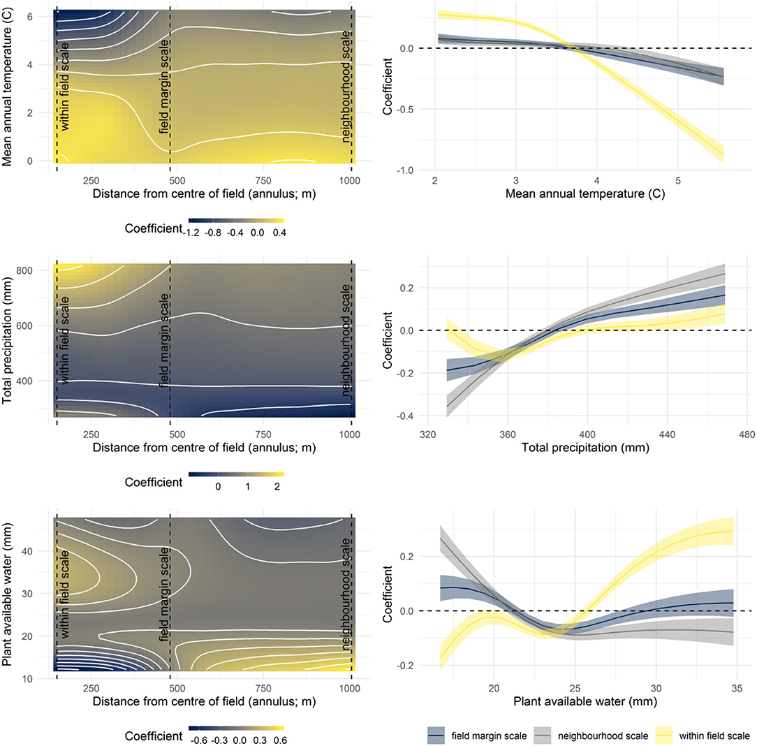
Figure 7. (Left) Bivariate coefficient functions for continuous environmental variables, where coefficients give deviations from the mean landscape complexity curve (Figure 3). (Right) The effect of the environmental variable across 95% of the observed distribution of that variable shown at three selected scales.

Mapping of a multi-scale index shows that there is geographic variation in the difference between the proportion of non-crop covers at the neighborhood and the within-field scales. Larger differences (darker colors; Figure 8) indicate that fields in these townships have much less non-crop cover than their neighborhoods. Smaller differences (lighter colors; Figure 8) suggest fields are closer to the local optimum for non-crop areas.

FIGURE 8

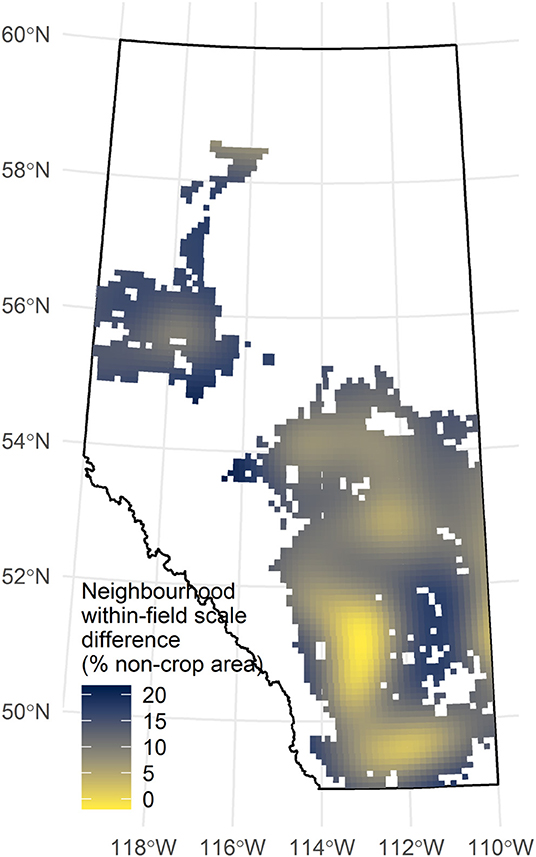
Figure 8. The difference in the predicted non-crop area between the within-field (150–400 m) and neighborhood (500–1,006 m) scales for each of the 2,480 survey townships with agricultural land. Model predictions exclude all environmental covariates but include spatial terms.

Discussion

This study demonstrated that there is considerable geographic variation in the proximity of non-crop areas to fields across Alberta's agricultural zone, and there remains capacity for growers and other land use decision makers to optimize this distribution. Analysis of landscape complexity curves revealed scale-dependent patterns in the proximity of non-crop areas to fields, such as the widespread occurrence of uncultivated field margins, and how land uses have been influenced by broad environmental gradients. These findings are considered in turn.

Potential for Changing Landscape Complexity

The capacity to introduce more non-crop land covers into fields, and therefore improve landscape complexity, can be seen by contrasting the proportions of non-crop area found within-fields to the neighborhood surrounding those fields (Figure 8). Non-crop area at the neighborhood scale can be understood as an estimate of the local potential for this quantity. Annuli at this scale sample from eight neighboring quarter sections, many of which may also be fields, effectively summarizing a region eight times the size of the focal field (Figure 1). The neighborhood scale, then, can be taken as a realistic potential proportion of non-crop area in the focal field because it captures neighboring land owners' willingness to allow those non-crop land covers to persist. It is also likely to be a correlate of the local expectation for crop productivity, given that neighboring growers would have an incentive to drain wetlands, clear trees and shrubs, remove perennial grasses, cultivate to fence lines or otherwise remove non-crop land covers from their fields, if that land could be used profitably for growing crops.

For example, the model suggests that within fields at location P (annulus = 150 m; Figures 4A,E) there is about 20% coverage in non-crop area, and there is also a similar coverage in the neighborhood (annulus = 995 m; Figures 4D,E). While 20% coverage suggests that non-crop covers are relatively common in fields, the more interesting observation is that there tend to be adjacent fields with similar non-crop proportions. This emerges as a flatter curve, and it is interpreted here as evidence that landscape complexity has reached its local potential; i.e., that land owners generally concur that 80% of the land should be in crops. The contrasting trend is evident at location T, where there is lower coverage of non-crop area within focal fields (about 5%) and higher coverage at the neighborhood scale (about 25%). Here fields have a low amount of non-crop area, but there is a large difference between the field and the neighborhood. This appears as a steeper curve, offering evidence that fields have less non-crop area than the local potential; i.e., that land owners differ markedly in how much land should be in crops.

Figure 8 (darker shades) therefore identifies parts of Alberta where agricultural land uses may be out of equilibrium with what the landscape can sustain, either because there may be more of each field in crop production than is optimal, or because there remains potential to further clear natural land covers for agriculture. The latter is probably the case in northern areas where twenty-first century clearing of boreal forest for agriculture is ongoing (north of 55°N; Bowen, 2002). However, the opportunity to clear more land is unlikely to be broadly important further south where agriculture has had an impact on the land since the late nineteenth century (Larmour, 2005).

The parts of the province that have the greatest difference at these two scales are those between 52°N and 55°N, after excluding the northern region and a region in south-central Alberta that is predominantly forage land (e.g., near point T; Figure 4). These latitudes are mostly in the parkland ecoregions, where prime agricultural land is abundant (Figure 2). There, growers may be able to leverage the collective wisdom of their neighbors to guide the return of non-crop areas to their fields. Or, in more concrete terms: marginal areas of fields that are currently cropped could be changed to non-crop vegetation; and forgoing production in these areas would mirror the decisions that neighbors have, on average, made regarding land use. This study, however, cannot provide any insight into how much non-crop land cover could be recovered. Rather it demonstrates that there are parts of the province where patterns in land use suggest the barriers doing so should be smaller than others.

Making the assumption that non-crop land covers in fields improve ecosystem services to agriculture (e.g., Rusch et al., 2016; Duarte et al., 2018; Vickruck et al., 2019), there is also the possibility that a small loss in crop area and therefore in farm returns, may be balanced by the improvement in the yields and profitability of crops on the remaining land. This can further reduce the risk associated with removing crop and replacing it with non-crop land covers.

Increasing non-crop land covers within fields could, in many parts of this region, be achieved by identifying marginal areas with relatively low productivity (e.g., measured in crop yield), removing them from production, and allowing other non-crop vegetation to re-establish. The proliferation of precision agricultural tools (e.g., yield monitors in harvesting equipment) should assist growers in identifying such sites (Mulla, 2013). These may be low spots in fields that have excess soil moisture or other poor soil conditions, or they may be near to other features that reduce productivity such as in the margins of wetlands where soils are poorly optimized for crop growth.

This study has not given any consideration to the class of non-crop cover and its association with landscape complexity, in part because this simplification aids interpretation. However, types of vegetation may differ in the ecosystem services they can provide to nearby crops, suggesting that regionally-targeted research on the benefits of establishing different vegetation classes is certainly appropriate. Equally, biasing re-establishment efforts toward perennial plants may better support carbon storage objectives (Hungate et al., 2017; Williams et al., 2018). However, the classes of vegetation already common at the neighborhood scale may be those that are the easiest to re-establish, and these may also be the species that naturally reclaim these sites without any intervention from land use decision-makers.

Patterns in the Proximity of Non-crop Area to Crops

Analysis of landscape complexity curves reveal field margins (400–500 m from field centers) as a common location for non-crop cover. These are evident as a peak at locations P, Q, R, S, and T (Figure 4E) at the scale that corresponds to the expected survey grid spacing. Geographically, the field margin effect is found throughout much of the region, with the notable exception of the extreme south of Alberta (annulus = 474 m; Figure 4B).

Field margins have been celebrated as a means to maintain non-crop areas in agricultural landscapes and to bring the ecosystem services they may provide close to fields with minimum loss of crop area (e.g., Marshall, 2002). In many cases these field margins are adjacent to roads or road allowances, which are public lands and are therefore at low risk of being changed to other land uses. Their widespread geographical distribution in Alberta represents an opportunity for regional policies that systematically promote their enhancement (e.g., by altering mowing regimes, or planting with native vegetation known to support ecosystem service provision; Kirmer et al., 2018).

Environmental Drivers of Landscape Complexity

Broad environmental gradients have played a role in shaping landscape complexity resulting in different patterns of non-crop area across scales. As might be expected, there is evidence that these gradients have influenced land use decisions, particularly the amount of clearing within fields and the density of fields at the neighborhood scale. Boreal ecoregions tended to have more non-crop area within fields (150–400 m; Figure 5) than the regional mean (Figure 3), perhaps reflecting the more recent clearing of these northern areas (Bowen, 2002) and the greater speed with which shrubs and trees can re-establish in the moisture and temperature regime of this part of the province. Grassland and parkland ecoregions registered at or less than the mean at the within field scale. The Mixed Grassland ecoregion had the most vegetation in field margins (400–500 m) while two ecoregions with significant tree cover (Mid-Boreal Uplands, and Boreal Transition) had the most non-crop area at neighborhood scales, reflecting the substantially lower amount of agricultural activity in these regions (Figure 5; Ecological Stratification Working Group, 1995).

Agricultural limitation classes demonstrated there has been more removal of vegetation within fields where there are fewer challenges to crop production in terms of the workability of the soil (Figure 6). Crop fields that have been successfully established in areas with severe limitations to agriculture suggest they are similar to the surrounding landscape in terms of non-crop area, and field margins are not distinguishable (e.g., marginal agriculture; Figure 6).

Temperature, precipitation and soil moisture variables enabled a directional assessment of how climatic variation is associated with landscape complexity patterns. Notably, locations with warmer temperatures and less soil moisture, conditions which favor prairie grassland species (Ecological Stratification Working Group, 1995), had less non-crop area within fields (Figure 7). The low frequency of woody vegetation in such dry prairie conditions means that clearing fields of all non-crop area is easier and less costly. Overall, the studies of environmental gradients indicate that landscape complexity is primarily under the control of land use decision-makers and not merely a result of local conditions, suggesting it is a matter of incentivizing these changes and not a problem simply of what the environment can sustain.

The multi-scale approach used in this study provided a flexible means to characterize landscape complexity as the proximity of non-crop features to crop fields. Interpretation of this model revealed that there is potential to increase landscape complexity by leveraging the natural potential in each region to support non-crop land cover and promoting practices that foster such vegetation, for example, on marginal or low-productivity sites within fields.

Data Availability Statement

The datasets generated for this study are available on request to the corresponding author.

Author Contributions

PG and MG were involved in the writing of the manuscript. PG was primarily responsible for the completion and interpretation of analyses. MG compiled the composite land cover data product on which this analysis was based.

Funding

This research was supported by research grants from Natural Sciences and Engineering Research Council (NSERC).

Conflict of Interest

The authors declare that the research was conducted in the absence of any commercial or financial relationships that could be construed as a potential conflict of interest.

References

Agriculture and Agri-Food Canada (2012). Land Capability for Agriculture. Canada Land Inventory (CLI). Retrieved from: http://www.data.gc.ca

Agriculture and Agri-Food Canada (2015). AAFC Annual Crop Inventory. Government of Canada. Retrieved from: http://open.canada.ca/

Google Scholar

Alberta Agriculture and Forestry (2017). Agriculture Statistics Yearbook.

Alberta Agriculture and Forestry (2018). Alberta Climate Information Service (ACIS). Retrieved from: https://agriculture.alberta.ca/acis/

Ancillotto, L., Ariano, A., Nardone, V., Budinski, I., Rydell, J., and Russo, D. (2017). Effects of free-ranging cattle and landscape complexity on bat foraging: implications for bat conservation and livestock management. Agric. Ecosyst. Environ. 241, 54–61. doi: 10.1016/j.agee.2017.03.001

CrossRef Full Text | Google Scholar

Asbjornsen, H., Hernandez-Santana, V., Liebman, M., Bayala, J., Chen, J., Helmers, M., et al. (2014). Targeting perennial vegetation in agricultural landscapes for enhancing ecosystem services. Renewable Agric. Food Syst. 29, 101–125. doi: 10.1017/S1742170512000385

CrossRef Full Text | Google Scholar

Birkhofer, K., Andersson, G. K. S., Bengtsson, J., Bommarco, R., Dänhardt, J., Ekbom, B., et al. (2018). Relationships between multiple biodiversity components and ecosystem services along a landscape complexity gradient. Biol. Conserv. 218, 247–253. doi: 10.1016/j.biocon.2017.12.027

CrossRef Full Text | Google Scholar

Boesing, A. L., Nichols, E., and Metzger, J. P. (2017). Effects of landscape structure on avian-mediated insect pest control services: a review. Landsc. Ecol. 32, 931–944. doi: 10.1007/s10980-017-0503-1

CrossRef Full Text | Google Scholar

Bommarco, R., Kleijn, D., and Potts, S. G. (2013). Ecological intensification: harnessing ecosystem services for food security. Trends Ecol. Evol. 28, 230–238. doi: 10.1016/j.tree.2012.10.012

PubMed Abstract | CrossRef Full Text | Google Scholar

Bowen, D. (2002). Agricultural expansion in Northern Alberta. Geogr. Rev. 92, 503–525. doi: 10.2307/4140932

CrossRef Full Text | Google Scholar

Bustamante, M., Robledo-Abad, C., Harper, R., Mbow, C., Ravindranat, N. H., Sperling, F., et al. (2014). Co-benefits, trade-offs, barriers and policies for greenhouse gas mitigation in the agriculture, forestry and other land use (AFOLU) sector. Glob. Change Biol. 20, 3270–3290. doi: 10.1111/gcb.12591

PubMed Abstract | CrossRef Full Text | Google Scholar

Chaplin-Kramer, R., O'Rourke, M. E., Blitzer, E. J., and Kremen, C. (2011). A meta-analysis of crop pest and natural enemy response to landscape complexity. Ecol. Lett. 14, 922–932. doi: 10.1111/j.1461-0248.2011.01642.x

PubMed Abstract | CrossRef Full Text | Google Scholar

Dalu, T., Wasserman, R. J., and Dalu, M. T. B. (2017). Agricultural intensification and drought frequency increases may have landscape-level consequences for ephemeral ecosystems. Glob. Change Biol. 23, 983–985. doi: 10.1111/gcb.13549

PubMed Abstract | CrossRef Full Text | Google Scholar

Doherty, K. E., Howerter, D. W., Devries, J. H., and Walker, J. (2018). Prairie Pothole Region of North America. In The Wetland Book, eds C. Finlayson, G. R. Milton, R. C. Prentice, and N. C. Davidson (Dordrecht: Springer), 1–10.

Google Scholar

Duarte, G. T., Santos, P. M., Cornelissen, T. G., Ribeiro, M. C., and Paglia, A. P. (2018). The effects of landscape patterns on ecosystem services: meta-analyses of landscape services. Landscape Ecol. 33, 1247–1257. doi: 10.1007/s10980-018-0673-5

CrossRef Full Text | Google Scholar

Ecological Stratification Working Group (1995). A National Ecological Framework for Canada.

Egli, L., Meyer, C., Scherber, C., Kreft, H., and Tscharntke, T. (2018). Winners and losers of national and global efforts to reconcile agricultural intensification and biodiversity conservation. Glob. Change Biol. 24, 2212–2228. doi: 10.1111/gcb.14076

PubMed Abstract | CrossRef Full Text | Google Scholar

Foley, J. A., Defries, R., Asner, G. P., Barford, C., Bonan, G., Carpenter, S. R., et al. (2005). Global Consequences of Land Use. Science. 309, 570–574.

PubMed Abstract | Google Scholar

Forman, R. T. T. (2009). Urban Ecology: Science of Cities. Cambridge.

Google Scholar

Godfray, H. C. J., Beddington, J. R., Crute, I. R., Haddad, L., Lawrence, D., Muir, J. F., et al. (2010). Food security: the challenge of feeding 9 billion people. Science 327, 812–818. doi: 10.1126/science.1185383

PubMed Abstract | CrossRef Full Text | Google Scholar

Goldsmith, J., Scheipl, F., Huang, L., Wrobel, J., Gellar, J., Harezlak, J., et al. (2019). Refund: Regression with Functional Data. R Package Version 0.1-17. Retrieved from: https://cran.r-project.org/package=refund.

Hungate, B. A., Barbier, E. B., Ando, A. W., Marks, S. P., Reich, P. B., van Gestel, N., et al. (2017). The economic value of grassland species for carbon storage. Science Adv. 3:e1601880. doi: 10.1126/sciadv.1601880

PubMed Abstract | CrossRef Full Text | Google Scholar

Karp, D. S., Frishkoff, L. O., Echeverri, A., Zook, J., Juárez, P., and Chan, K. M. A. (2018). Agriculture erases climate-driven β-diversity in Neotropical bird communities. Glob. Change Biol. 24, 338–349. doi: 10.1111/gcb.13821

PubMed Abstract | CrossRef Full Text | Google Scholar

Kirmer, A., Rydgren, K., and Tischew, S. (2018). Smart management is key for successful diversification of field margins in highly productive farmland. Agric. Ecosyst. Environ. 251, 88–98. doi: 10.1016/j.agee.2017.09.028

CrossRef Full Text | Google Scholar

Kleijn, D., Kohler, F., Báldi, A., Batáry, P., Concepción, E. D., Clough, Y., et al. (2009). On the relationship between farmland biodiversity and land-use intensity in Europe. Proc. Biol. Sci. 276, 903–909. doi: 10.1098/rspb.2008.1509

PubMed Abstract | CrossRef Full Text | Google Scholar

Kokoszka, P. and Reimherr, M. (2017). Introduction to Functional Data Analysis. New York, NY: CRC Press.

Google Scholar

Lamb, A., Green, R., Bateman, I., Broadmeadow, M., Bruce, T., Burney, J., et al. (2016). The potential for land sparing to offset greenhouse gas emissions from agriculture. Nature Clim. Change 6, 488–492. doi: 10.1038/nclimate2910

CrossRef Full Text | Google Scholar

Landis, D. A. (2017). Designing agricultural landscapes for biodiversity-based ecosystem services. Basic Appl. Ecol. 18, 1–12. doi: 10.1016/j.baae.2016.07.005

CrossRef Full Text | Google Scholar

Larmour, J. (2005). Laying Down the Lines: A History of Land Surveying in Alberta. Brindle and Glass. Victoria, BC.

Google Scholar

Laurance, W. F., Sayer, J., and Cassman, K. G. (2014). Agricultural expansion and its impacts on tropical nature. Trends Ecol. Evol. 29, 107–116. doi: 10.1016/j.tree.2013.12.001

PubMed Abstract | CrossRef Full Text | Google Scholar

Marshall, E. J. P. (2002). Introducing field margin ecology in Europe. Agric. Ecosyst. Environ. 89, 1–4. doi: 10.1016/S0167-8809(01)00314-0

CrossRef Full Text | Google Scholar

Mulla, D. J. (2013). Twenty five years of remote sensing in precision agriculture: key advances and remaining knowledge gaps. Biosyst. Eng. 114, 358–371. doi: 10.1016/j.biosystemseng.2012.08.009

CrossRef Full Text | Google Scholar

Phalan, B., Onial, M., Balmford, A., and Green, R. E. (2011). Reconciling food production and biodiversity conservation: land sharing and land sparing compared. Science 333, 1289–1291. doi: 10.1126/science.1208742

PubMed Abstract | CrossRef Full Text | Google Scholar

Rusch, A., Chaplin-Kramer, R., Gardiner, M. M., Hawro, V., Holland, J., Landis, D., et al. (2016). Agricultural landscape simplification reduces natural pest control: a quantitative synthesis. Agric. Ecosyst. Environ. 221, 198–204. doi: 10.1016/j.agee.2016.01.039

CrossRef Full Text | Google Scholar

Smith, P. (2014). Do grasslands act as a perpetual sink for carbon? Glob. Change Biol. 20, 2708–2711. doi: 10.1111/gcb.12561

PubMed Abstract | CrossRef Full Text | Google Scholar

Statistics Canada (2016). Census of Agriculture. Statistics Canada. Ottawa, ON.

Google Scholar

Tscharntke, T., Tylianakis, J. M., Rand, T. A., Didham, R. K., Fahrig, L., Batáry, P., et al. (2012). Landscape moderation of biodiversity patterns and processes - eight hypotheses. Biol. Rev. 87, 661–685. doi: 10.1111/j.1469-185X.2011.00216.x

PubMed Abstract | CrossRef Full Text | Google Scholar

Vickruck, J. L., Best, L. R., Gavin, M. P., Devries, J. H., and Galpern, P. (2019). Pothole wetlands provide reservoir habitat for native bees in prairie croplands. Biol. Conserv. 232, 42–50. doi: 10.1016/j.biocon.2019.01.015

CrossRef Full Text | Google Scholar

Williams, D. R., Phalan, B., Feniuk, C., Green, R. E., and Balmford, A. (2018). Carbon storage and land-use strategies in agricultural landscapes across three continents. Curr. Biol. 28, 2500–2505. doi: 10.1016/j.cub.2018.05.087

PubMed Abstract | CrossRef Full Text | Google Scholar

Wood, S. N. (2017). Generalized Additive Models: an Introduction With R. New York, NY: CRC Press.

Google Scholar