Applying Multi-Layer Artificial Neural Network and Mutual Information to the Prediction of Trends in Dissolved Oxygen

Predicting trends in water quality plays an essential role in the field of environmental modeling. Though artificial neural networks (ANN) have been involved in predicting water quality in many studies, the prediction performance is highly affected by the model's inputs and neural network structure. Many researchers selected water quality variables based on Pearson correlation. However, this kind of method can only capture linear dependencies. Moreover, when dealing with multivariate water quality data, ANN with the single layer and few numbers of units show difficulties in representing complex inner relationships between multiple water quality variables. Hence, in this paper we propose a novel model based on multi-layer artificial neural networks (MANN) and mutual information (MI) for predicting the trend of dissolved oxygen. MI is used to evaluate and choose water quality variables by taking into account the non-linear relationships between the variables. A MANN model is built to learn the levels of representations and approximate complex regression functions. Water quality data collected from Baffle Creek, Australia was used in the experiment. Our model had around 0.95 and 0.94 R² scores for predicting 90 or 120 min ahead of the last observed data in the wet season, which are much higher than the typical ANN model, support vector regressor (SVR) and linear regression model (LRM). The results indicate that our MANN model can provide accurate predictions for the trend of DO in the upcoming hours and is a useful supportive tool for water quality management of the aquatic ecosystems.

1. Introduction

Increasing human populations together with the progression of climate change is leading to unprecedented changes in aquatic ecosystems. Climate change is expected to cause water quality decline, with negative effects on aquatic organisms (Gillanders et al., 2011). In this context, the development of reliable water quality predictions is critical to improve management of aquatic ecosystems. Traditionally, mechanistic models have been used to predict water quality (Silva et al., 2014). However, the success of these predictions depends on how tightly the physical environment drives the water quality of the system (Robson, 2014). Most recently, data-driven models have provided successful in predicting water quality. For instance, ANN have been used to accurately predict anomalies in surface water quality (Shi et al., 2018). ANN have been also applied to successfully predict dissolved oxygen (DO) in rivers (Sarkar and Pandey, 2015) and aquaculture prawn ponds (Dabrowski et al., 2018).

Dissolved oxygen is a key indicator of the health of aquatic ecosystems. The level of DO in water determines the quality and quantity of habitat available to aquatic organisms. Low DO levels can cause aquatic organisms to experience acute stress and eventually lead to their mortality (Gillanders et al., 2011). In addition, changes in DO alter biochemical cycling and the release of nutrients from the sediments. Phosphorus release from the sediments can occur in short time-scales with the onset of low oxygen levels close the sediment-water interface (Vilas et al., 2018). Thus, short-term predictions of DO can guide the implementation of management actions to maintain good water quality conditions.

Dissolved oxygen levels are driven by the physical environment and complex biogeochemical processes (Vilas et al., 2017). As the solubility of oxygen in water depends on the temperature of water, water temperature is an important driver of the concentration of DO. Dissolved oxygen is also driven by the abundance of primary producers. Thus, data-driven predictions need to consider variables that account for both the physical and biogeochemical environment.

Even though a number of data-driven models are proposed for DO prediction, there has been little focus on developing a systematic way to select appropriate inputs (Wu et al., 2014). For instance, Sarkar and Pandey (2015) combined data sets obtained from three different monitoring stations and used them as input to the ANN model, without implementing any feature selection method. In addition, Shi et al. (2018) used seven surface water quality variables in their ANN based model to predict water quality anomalies, also without using any variable analysis method. In addition, merely including all available variables may contain irrelevant or redundant information, which can decrease the performance of the data-driven model.

While many studies select water quality variables based on Pearson correlation, this method can only deal with linear dependencies. Beside this, some researchers (Antanasijević et al., 2014; Burchard-Levine et al., 2014; Alizadeh and Kavianpour, 2015; Piotrowski et al., 2015) have evaluated the combinations of inputs based on the model's outputs. This trial and error idea needs to test all possible groups of inputs by building a number of predictive models, which can be very inefficient when dealing with large volumes of water quality datasets.

In recent years, artificial neural networks have shown great flexibility in modeling and forecasting non-linear dynamic time series processes. In the field of environmental and water resources modeling, different types of ANN models such as radial basis function network (Deng et al., 2014) and multi-layer perceptron Najah et al. (2013) have been used. However, most of these studies (Cordoba et al., 2014; Kim and Seo, 2015; Csábrági et al., 2017) have used shallow neural network structures with few hidden units and single layer. These models cannot learn multi levels of representation from the water quality inputs because of limited number of hidden layers.

Hence, we proposed a novel approach for dissolved oxygen prediction that enables: (a) the selection of best-related water quality variables for predicting DO, and (b) the prediction of short-term (90–120 min) changes in DO concentration. In our predictive model, a mutual information based feature selection strategy is designed to evaluate the association between water quality variables. Moreover, a MANN is used to thoroughly learn levels of representations and approximate complex non-linear relationships within multivariate time series data.

2. Materials and Methods

2.1. Study Area and Water Quality Data

The water quality of Baffle Creek is studied as an example. Baffle Creek estuary system is one of the largest estuaries in Queensland, Australia and has a catchment area of approximately 3,000 km². The time series of water quality data has been collected by the in situ near real-time monitoring sensors (YSI, Model 6600) deployed 16 km from the mouth of Baffle Creek (Figure 1). Readings of water temperature, electric conductivity (EC), pH, dissolved oxygen (DO), turbidity, and chlorophyll-a (Chl-a) were recorded every half hour at 0.2 m below water surface¹.

FIGURE 1

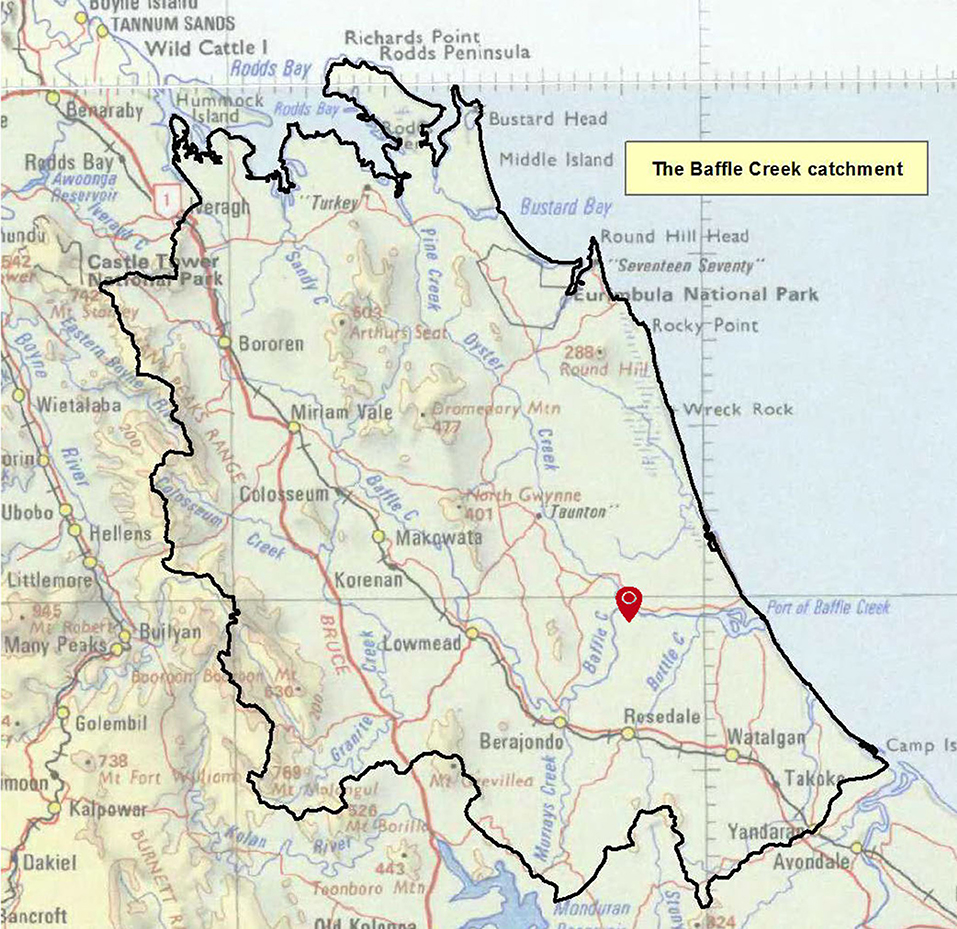
Figure 1. Baffle Creek catchment area and the water quality monitoring station.

Climate in the north area of Queensland is characterized by wet and dry season patterns. In general, the wet season starts from November to April and the dry season starts from May to October. The data set used in this paper contained 17,530 observations measured between 1/11/2013 and 31/10/2014. For the wet season, training data included first 5 months' observations (7,248 records) and testing data included last 1 month's observations (1,440 records). For the dry season, training data included first 5 months' observations (7,354 records) and testing data included last 1 month's observations (1,488 records). A summary of the water quality variables is shown in Table 1.

TABLE 1

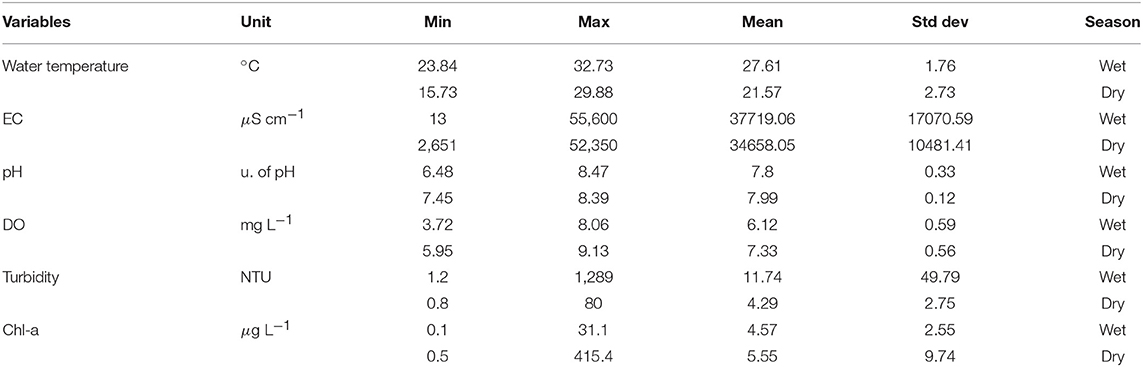
Table 1. Details of water quality data.

Water quality variables such as EC, turbidity and Chl-a have a wide range of values, particularly during the wet season (Table 1) and thus a predictive model should have the capability to handle such a large variance in the data. Moreover, water quality variables show different ranges between the wet and dry seasons. For example, the minimum value of EC is only 13 μS cm⁻¹ in the wet season, which is over 200 times smaller than that in the dry season. Hence, the performance of predictive model needs to be evaluated both on the wet and dry seasons to guarantee good generalization of the proposed method.

Figure 2 illustrates the data distribution of 6 physochemical variables listed in Table 1. It is clear that the distribution of most water quality variables is not symmetric. Values of water temperature, turbidity and Chl-a are most concentrated toward the lower end of the axis with some extreme large values. On the contrary, variables like pH and EC have few small values and most of the data have higher values. The uneven distribution of water quality data in Figure 2 is also a challenge for learning the changing patterns for different water quality variables. Hence, neural network can be a suitable method in modeling water quality variables because it supports the non-linear transformations and does not rely on stationary data series.

FIGURE 2

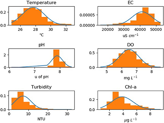
Figure 2. Histogram of 6 physiochemical parameters.

Normalizing original data boosts the performance of ANN models significantly. In this study, we choose the min-max data normalization method to preprocess all the inputs. The min-max normalization is shown in Equation 1:

$\begin{array}{ll}Î=\frac{I}{I_{max}-I_{min}},& (1)\end{array}$

where I is the original value and Î is the normalized value.

2.2. Mutual Information Based Feature Selection

Feature selection is an important issue in machine learning and has been widely investigated. Effective feature selection results in a better and simpler understanding of the process that generates the data (Vergara and Estévez, 2013).

2.2.1. Mutual Information

Similarity measures such as the Pearson correlation coefficient (Pearson, 1895) are widely used in evaluating the relationships between different features in many water quality prediction studies. Though the computing of Pearson correlation can easily to be scaled up to large data sets, the correlation is a measure of the linear relationship between random variables.

In this study, we choose to select water quality features based on their "mutual information" content. The mutual information is a measure of the amount of information that one random variable has about another variable (Kraskov et al., 2004). From information theory, formally, the MI is defined as follows:

$\begin{array}{ll}I(X,Y)={\displaystyle \iint dxdy\mu (x,y)log\frac{\mu (x,y)}{{\mu }_x(x){\mu }_y(y)}.}& (2)\end{array}$

where the marginal densities of X and Y are μ_x(x) = ∫dyμ(x, y) and μ_y(y) = ∫dxμ(x, y).

Unlike correlation coefficients, MI is more general and contains information about all linear and non-linear dependencies. The non-binning MI estimator proposed by Ross (2014) was calculated for each input feature (Table 2).

TABLE 2

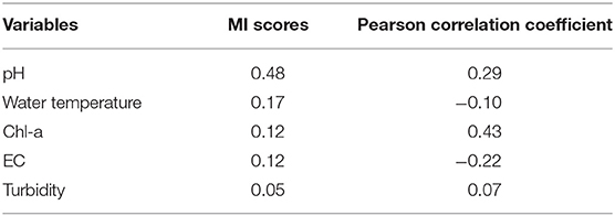
Table 2. Correlation scores for each water quality variable against do.

MI scores ranked in Table 2 show how much information each variable has about DO. Among these variables, turbidity has much lower MI score and EC has the second last MI score. Water temperature and Chl-a have similar MI scores and pH shows a significant high MI score. Based on the MI definition in Equation 2, high mutual information indicates a high relevance between the water quality variable and DO. In this case, both EC and turbidity are omitted in predicting DO.

Additionally, the Pearson correlation coefficient is also calculated for each water quality parameter. Water temperature, EC, and Turbidity show extremely low correlation with DO based on the Pearson correlation coefficient. Hence, only pH and Chl-a are selected for predicting DO. In the experiment section, the predictive performance will be evaluated for these two feature selection algorithms.

2.2.2. Correlation Between Water Quality Variables

In this subsection, we analyzed the patterns of water quality variables (water temperature, EC, pH, turbidity, and Chl-a) and compared them with those of DO. This allowed us to demonstrate the validity of the MI based feature selection strategy and explain the reason of selecting pH, water temperature and Chl-a for predicting the trend of DO.

In the left column of Figure 3, the daily changes of 5 water quality variables are shown. The temporal change of DO is also added to each subfigure for comparison. Considering variables listed in Table 1 all have different units, we scale their values by using the min-max normalization (Equation 1) to make the comparison clear. Correspondingly, the relationships between water quality variables and DO are illustrated in the right scatterplots.

FIGURE 3

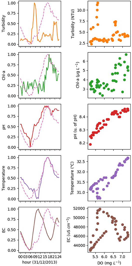
Figure 3. Daily changes of 5 physochemical parameters and the correlations with DO. Solid and dotted lines in left column represent water quality parameters and DO, respectively. Relationships between water quality parameters and DO are illustrated in the right scatterplots. All the water quality parameters have been scaled by using the min-max normalization in Equation 1.

In Figure 3, DO increases during the day and declines during night, with maximum value occurring at 5 p.m. in the afternoon. Chl-a, pH, and water temperature show significant positive correlation with DO. They all follow a similar pattern than DO, decreasing during the night and increasing during the day. Changes in DO in time are a result of physical and biogeochemical processes. On a diurnal time-scale, DO increases during the day as a result of the photosynthetic activity of primary producers (i.e., phytoplankton) and decreases during the night due to respiration. In addition, photosynthesis and respiration drive the diel changes in dissolved carbon dioxide (CO₂) concentrations that induce the daily variation of pH (Zang et al., 2010). All of these processes are affected by the temperature of the water.

On contrary, the daily trends of turbidity and EC do not show clear relationship with that of DO. For example, the peak value of turbidity is attained early in the day and for most of the time turbidity remains in a low level. In Table 2, EC and turbidity also have low MI scores. This demonstrates that MI-based feature selection is likely better suited to select water quality variables for predicting the trend of DO than the Pearson correlation coefficient. The Pearson correlation coefficient disregards water temperature and EC, which may affect the predictive performance of the model.

2.3. Multi-Layer Artificial Neural Network With Dropout

Artificial neural network models input data to higher level abstraction by using an architecture with many hidden layers composed of linear and non-linear transformations. In this paper, a multi-layer feedforward neural network with dropout mechanism is used in building our water quality predictive model.

2.3.1. Multi-Layer FeedForward Neural Network

A multi-layer feedforward neural network has an input layer of source nodes and an output layer of neurons. In addition to these two layers, it has multiple layers of hidden units. The hidden units extract important features contained in the input data and the multiple hidden layers provide the capability to learn representations of data with multiple levels of abstraction. The structure of the MANN used is illustrated in Figure 4.

FIGURE 4

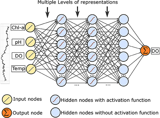
Figure 4. MANN for predicting DO.

As it is shown in Figure 4, the number of units in the input layer is p*n, where p is the number of selected variables and n is the number of historical observations. In this way, models can accept time series water quality data with multiple variables. Also, a fully connected layer with linear regression is added in the end to output single prediction value.

One of the challenges in building neural networks with multiple layers is updating the weights of the networks. In our model, the stochastic gradient descent algorithm (SGD) (Robbins and Monro, 1951) is used to train the MANN. During the training process, inputs data is fed into the network to optimize the weights between units. Adjustment of the weights between units in different layers is done by backward propagation of the error during training phase. The network adjusts the value of the weights to reduce the difference between the output and target values (Sharma and Venugopalan, 2014). The error is minimized across many training loops until we get the MANN with required accuracy.

2.3.2. Dropout

When a MANN is trained on a relatively small training set, it typically performs poorly on held-out test data. In the field of water quality modeling, considering the difficulties of monitoring site deployment and the limitation of sensor hardware, it is hard to get large data sets, spanning the period of interest.

Dropout is a technique that can both prevent overfitting and provide a way of approximately combining many different neural network architectures efficiently (Hinton et al., 2012). Dropout refers to dropping out units in a neural network, which means temporarily removing it from the network, along with all its incoming and outgoing connections. Dahl et al. (2013) proposed an equation to compute the activation y_t of the layer t of the net during forward propagation. Here the activation y_t indicates the status of all the activations of the hidden units in a given layer:

$\begin{array}{ll}{\text{y}}_t=f(\frac{1}{1-r}{\text{y}}_{t-1}*\text{m}\text{W}+\text{b}),& (3)\end{array}$

where f is the activation status for the tth layer, W and b are, respectively the weights and biases for the layer, * denotes element-wise multiplication, and m is a binary mask from Bernoulli(1−r) indicating which activations are not dropped out.

By using dropout technique, each training example can thus be viewed as providing gradients for a different, randomly sampled architecture. For example, in Figure 5, a number of hidden units are inactivated during training so the ANN's structure is changed in each training phase. Comparing training a model without dropout, applying dropout can prevent the hidden units from co-adapting too much. The final neural network efficiently represents a huge ensemble of neural networks, with good generalization capability (Dahl et al., 2013).

FIGURE 5

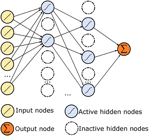
Figure 5. Neural network with dropout.

2.4. Water Quality Prediction Model

In this subsection, we developed our water quality predictive model by integrating MI and MANN with dropout mechanism.

In our water quality predictive model (Figure 6), data collected from monitoring sites is analyzed first, which gives us statistical overview about the water quality variables. Then, the MI feature selection is implemented to pick up most related variables. After rescaling input variables based on min-max normalization (Equation 1), the input samples are created based on the selected variables and the historical number of observations we choose. Finally, the MANN model with dropout mechanism is used to output the predictive value.

FIGURE 6

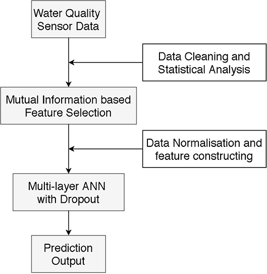
Figure 6. Water quality prediction model proposed in this paper.

3. Results and Discussion

3.1. Experiment Setting

In this study we implemented 90 min (3 time steps) and 120 min (4 time steps) forecasts of DO for both wet and dry seasons. For the inputs, we used the last 12 water quality observations of water temperature, pH, Chl-a and DO as the MANN model's inputs.

The structure of the neural network also needs to be determined. This structure, known as hyperparameters, includes the number of hidden layers, the number of units in each layer, activation function, between others. Optimizing the hyperparameters is critically important for the model's performance. In this experiment, by both considering the size of water quality data set and the model's training time, we finally got the optimized parameters shown in Table 3.

TABLE 3

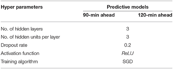
Table 3. Hyperparameters of our proposed MANN models.

We chose SGD algorithm and ReLU activation function (Nair and Hinton, 2010) together for our MANN model. ReLU is a computationally efficient activation function because it involves simpler mathematical operations, which can accelerate the training process when we train ANN with multiple layers. Moreover, the ReLU activation function has range [0, ∞]. This property makes it support model positive real value, which is important in processing water quality parameters.

All the experiments are evaluated on the CSIRO HPC server with 1 Core Xeon E5-2690 and 32 GB memory. The MANN and ANN are built on the Keras neural network framework (Chollet et al., 2015). The SVR and LRM are implemented on the scikit-learn machine learning framework (Pedregosa et al., 2011).

3.2. Evaluation Criteria

In order to measure the performance of the predictive model, we used the mean absolute error (MAE), the coefficient of determination (R²) and the root mean square error (RMSE). They are defined as:

$\begin{array}{ll}MAE=\frac{1}{n}{\displaystyle \sum _{i=1}^n}|f_i-{\widehat{f}}_i|& (4)\end{array}$

$\begin{array}{ll}{R}^2=1-\frac{{\displaystyle {\sum }_{i=1}^n}{(f_i-{\widehat{f}}_i)}^2}{{\displaystyle {\sum }_{i=1}^n}{(f_i-\overline{f_i})}^2}& (5)\end{array}$

$\begin{array}{ll}RMSE=\sqrt{\frac{1}{n}{\displaystyle \sum _{i=1}^n}{\left(|f_i-{\widehat{f}}_i|\right)}^2}& (6)\end{array}$

where f_i is the observed value, ${\widehat{f}}_i$ is the predicted value and $\overline{f_i}=\frac{1}{n}\sum _{i=1}^n{f}_i$.

3.3. Prediction Results

Figure 7 shows the prediction of DO in both wet and dry seasons. It is clear that the concentration of DO has stronger variation in the wet season (Figure 7A) than it is in the dry season (Figure 7B). In the wet season, the concentration of DO increases from around 4.0 mg L⁻¹ to nearly 7.5 mg L⁻¹ within the first month and thereafter fluctuates between 5.5 and 7.0 mg L⁻¹. During this period, our MANN model is effective in predicting the diurnal variation pattern as well as the long term variability. Also, the MANN model has a quick response when DO concentrations start to increase or decrease. This means the MANN model is very sensitive when the trend of DO begins to change.

FIGURE 7

Figure 7. DO prediction in both the wet and dry seasons. (A) 90 min ahead DO prediction in the wet season (1/4/2014-30/4/2014). (B) 90 min ahead DO prediction in the dry season (1/10/2014-31/10/2014).

Similarly, our MANN model performs well in predicting the concentration of DO in the dry season (Figure 7B). In the dry season, the concentration of DO changes within a small range between 6.2 and 7.0 mg L⁻¹. The reason behind this is that rainfall affects the concentration of DO significantly and the rainfall frequency during the dry season is low.

Moreover, Figure 8 shows the details between the prediction and measured value in 4 different experimental cases. The R² of wet season testing data are 0.95 and 0.94, respectively, suggesting good fit of the model to the water quality dataset used. Additionally, the R² of dry season testing data are 0.88 and 0.80. This result indicates a stable predictive capability of our MANN model.

FIGURE 8

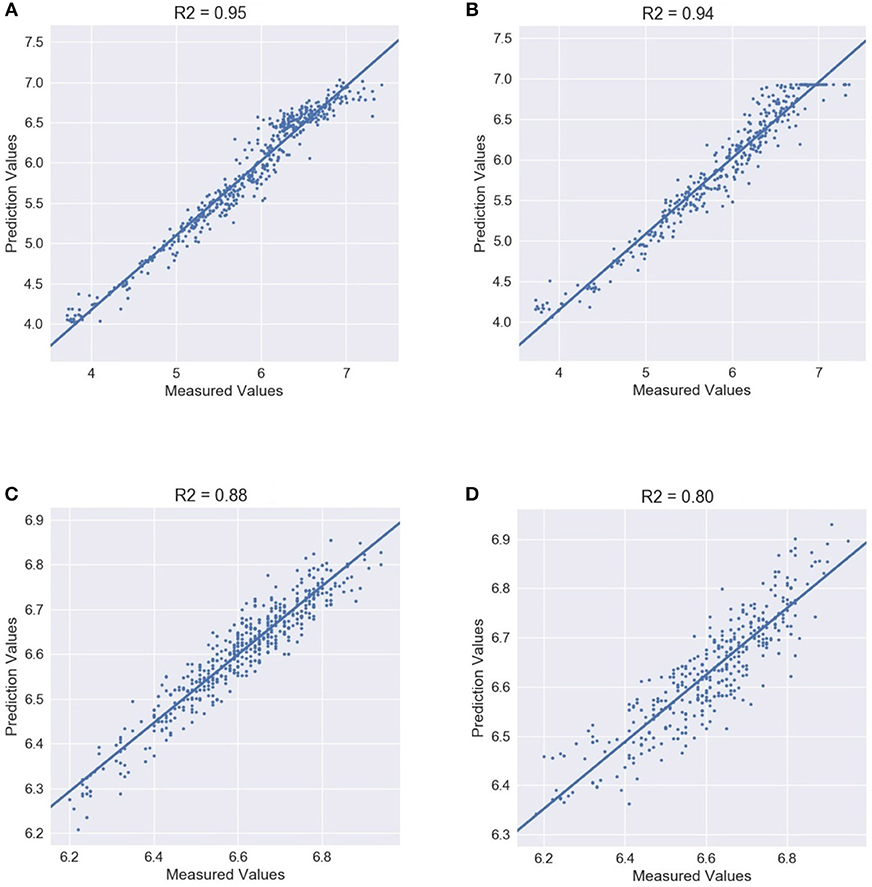
Figure 8. 90/120 min ahead prediction and measured value comparison. Wet-90 represents the experimental case for 90 min ahead prediction for the wet season. Other cases are named in the same way. (A) Wet-90 DO prediction. (B) Wet-120 DO prediction. (C) Dry-90 DO prediction. (D) Dry-120 DO prediction.

We also compared the performance of our MANN model with the single layer ANN, SVR and LRM. The ANN model used in this experiment is designed to have one hidden layer and nine hidden units, which equals the total number of hidden units of our MANN model. For the SVR model, we use the grid search to get the best parameters.

In addition, to reveal the benefits of applying dropout mechanism and the MI feature selection, we compared our model with another two models MANN-Dropout and MANN+Pearson. In the MANN-Dropout, the dropout layer was removed from the original MANN model. In the MANN+Pearson, we used the Pearson correlation coefficient instead of the MI to select input variables.

Our model is proved to be more accurate than the single layer ANN, SVR, and LRM in all experiments (Figure 9). For example in the wet-120 experiment, our proposed model has 0.19 RMSE score, 0.14 MAE score and 0.94 R² score. Though ANN performs better than SVR in this case, it can only achieve 0.35 RMSE score, 0.25 MAE score and 0.81 R² score. Our MANN model can achieve even higher accuracy when predicting 90 min ahead DO in the wet season. In the dry season, our MANN model also has the best performance. It achieves 0.05 RMSE score and 0.04 MAE score in the 90 min ahead prediction, which indicates very high prediction accuracy.

FIGURE 9

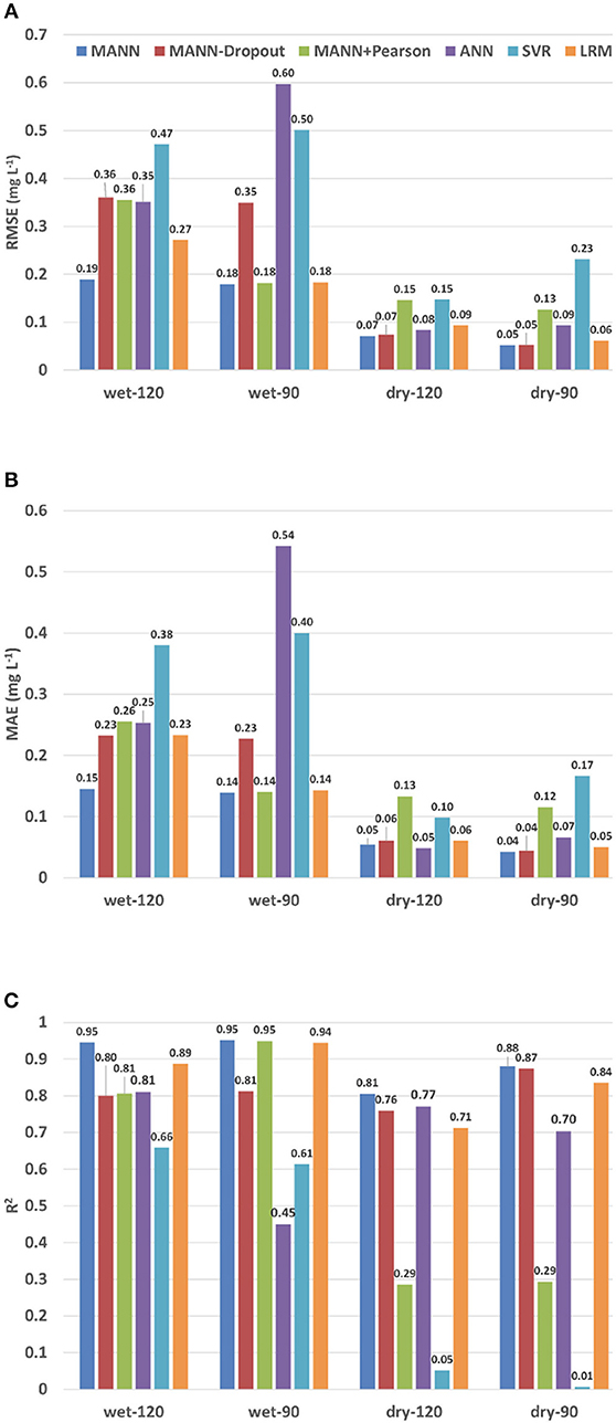
Figure 9. Performance evaluation for 6 different models. Wet-90 represents the experimental case for 90 min ahead prediction for the wet season. Other cases are named in the same way. (A) RMSE of 6 different models in 4 experimental cases. (B) MAE of 6 different models in 4 experimental cases. (C) R² of 6 different models in 4 experimental cases.

The MANN-Dropout and the MANN+Pearson performed better than the ANN, SVR, and LRM in most cases. However, they still yield worse predictions than the original MANN for these cases. For example, our MANN had an R² score of 0.81 in the dry-120, while the MANN-Dropout and the MANN+Pearson had a lower R² score of 0.76 and 0.29, respectively.

Without adding the dropout layer, the MANN-Dropout tends to overfit with the training datasets. Therefore, when applying the well-trained model to the testing dataset, it could not achieve high performance as we expected. For the MANN+Pearson, only two water quality parameters were chosen as inputs (Table 2). Based on the correlations between the measured variables and DO analyzed in subsection 2.2.2, water temperature and EC also have a strong correlation with the concentration of DO. Thus, removing that information can decrease the accuracy in predicting the DO concentration.

Accurate predictions of DO concentrations can help better manage aquatic ecosystems. Low DO concentrations can lead to the mortality of aquatic organisms and the release of nutrients from the sediments (Gillanders et al., 2011; Vilas et al., 2018). The increase of nutrients in the water column can in turn promote phytoplankton blooms which impair the health of aquatic ecosystems (Vilas et al., 2018). Accurate short-term predictions of DO, such as those derived in this study, can be useful to trigger the implementation of management practices aiming at reestablishing oxic conditions in the water column. For instance, short-term predictions can be useful to activate an aerator when oxygen levels are predicted to fall below a threshold value. Thus, short-term predictions of DO can inform cost effective solutions to prevent water quality crises. The model and methodology presented here can be applied to DO prediction in other aquatic ecosystems such as lakes and rivers.

4. Conclusion

We proposed a water quality predictive model based on a multi-layer feed-forward neural network with the mutual information feature selection. We also evaluated the performance of our model on water quality data collected from Baffle Creek. Unlike most of the existing methods that are built on a shallow neural network, the proposed MANN model was successful in capturing non-linear temporal correlations for the trend of DO and our method was more accurate compared to the benchmark methods.

Future investigations need to assess how climate data, rainfall and soil information could be included to improve the model's performance. In addition, future investigations need to consider how ANN perform against other mechanistic or statistical models, such as time series models.

Author Contributions

YZ conceived and designed the analysis, collected the data, performed the analysis, wrote the paper, and discussed the results and contributed to the final manuscript. PF provided critical feedback, verified the analytical methods, discussed the results and contributed to the final manuscript. PT verified the analytical methods, supervise the project, discussed the results and contributed to the final manuscript. MV helped re-design the experiments, helped shape the research, analysis and manuscript, and discussed the results and contributed to the final manuscript.

Funding

This work was conducted within the Digiscape Future Science Platform leading by CSIRO.

Conflict of Interest Statement

The authors declare that the research was conducted in the absence of any commercial or financial relationships that could be construed as a potential conflict of interest.

Footnote

1. ^Ambient Estuarine Water Quality Monitoring Data. Available online at: https://data.qld.gov.au/dataset (Accessed November 20, 2017).

References

Alizadeh, M. J., and Kavianpour, M. R. (2015). Development of wavelet-ANN models to predict water quality parameters in hilo bay, pacific ocean. Mar. Pollut. Bull. 98, 171–178. doi: 10.1016/j.marpolbul.2015.06.052

PubMed Abstract | CrossRef Full Text | Google Scholar

Antanasijević, D., Pocajt, V., Perić-Grujić, A., and Ristić, M. (2014). Modelling of dissolved oxygen in the danube river using artificial neural networks and monte carlo simulation uncertainty analysis. J. Hydrol. 519, 1895–1907. doi: 10.1016/j.jhydrol.2014.10.009

CrossRef Full Text | Google Scholar

Burchard-Levine, A., Liu, S., Vince, F., Li, M., and Ostfeld, A. (2014). A hybrid evolutionary data driven model for river water quality early warning. J. Environ. Manag. 143, 8–16. doi: 10.1016/j.jenvman.2014.04.017

PubMed Abstract | CrossRef Full Text | Google Scholar

Chollet, F. (2015). Keras. Available online at: https://keras.io

Cordoba, G. C., Tuhovčák, L., and Tauš, M. (2014). Using artificial neural network models to assess water quality in water distribution networks. Procedia Eng. 70, 399–408. doi: 10.1016/j.proeng.2014.02.045

CrossRef Full Text | Google Scholar

Csábrági, A., Molnár, S., Tanos, P., and Kovács, J. (2017). Application of artificial neural networks to the forecasting of dissolved oxygen content in the hungarian section of the river danube. Ecol. Eng. 100, 63–72. doi: 10.1016/j.ecoleng.2016.12.027

CrossRef Full Text | Google Scholar

Dabrowski, J. J., Rahman, A., George, A., Arnold, S., and McCulloch, J. (2018). “State space models for forecasting water quality variables: an application in aquaculture prawn farming,” in Proceedings of the 24th ACM SIGKDD International Conference on Knowledge Discovery & Data Mining (London), 177–185.

Google Scholar

Dahl, G. E., Sainath, T. N., and Hinton, G. E. (2013). “Improving deep neural networks for lvcsr using rectified linear units and dropout,” in International Conference on Acoustics, Speech and Signal Processing (ICASSP) (Vancouver, BC: IEEE), 8609–8613.

Google Scholar

Deng, W., Wang, G., Zhang, X., Guo, Y., and Li, G. (2014). “Water quality prediction based on a novel hybrid model of arima and rbf neural network,” in 3rd International Conference on Cloud Computing and Intelligence Systems (CCIS) (Shenzhen: IEEE).

Google Scholar

Gillanders, B. M., Elsdon, T. S., Halliday, I. A., Jenkins, G. P., Robins, J. B., and Valesini, F. J. (2011). Potential effects of climate change on australian estuaries and fish utilising estuaries: a review. Mar. Fresh. Res. 62, 1115–1131. doi: 10.1071/MF11047

CrossRef Full Text | Google Scholar

Hinton, G. E., Srivastava, N., Krizhevsky, A., Sutskever, I., and Salakhutdinov, R. R. (2012). Improving neural networks by preventing co-adaptation of feature detectors. arXiv:1207.0580.

Google Scholar

Kim, S. E., and Seo, I. W. (2015). Artificial neural network ensemble modeling with conjunctive data clustering for water quality prediction in rivers. J. Hydro Environ. Res. 9, 325–339. doi: 10.1016/j.jher.2014.09.006

CrossRef Full Text | Google Scholar

Kraskov, A., Stögbauer, H., and Grassberger, P. (2004). Estimating mutual information. Phys. Rev. E 69, 066138. doi: 10.1103/PhysRevE.69.066138

PubMed Abstract | CrossRef Full Text | Google Scholar

Nair, V., and Hinton, G. E. (2010). “Rectified linear units improve restricted boltzmann machines,” in Proceedings of the 27th International Conference on International Conference on Machine Learning ICML'10, (Omnipress), 807–814.

Google Scholar

Najah, A., El-Shafie, A., Karim, O. A., and El-Shafie, A. H. (2013). Performance of ANFIS versus MLP-NN dissolved oxygen prediction models in water quality monitoring. Environ. Sci. Pollut. Res. 21, 1658–1670. doi: 10.1007/s11356-013-2048-4

PubMed Abstract | CrossRef Full Text | Google Scholar

Pearson, K. (1895). Note on regression and inheritance in the case of two parents. Proc. R. Soc. Lond. 58, 240–242. doi: 10.1098/rspl.1895.0041

CrossRef Full Text | Google Scholar

Pedregosa, F., Varoquaux, G., Gramfort, A., Michel, V., Thirion, B., Grisel, O., et al. (2011). Scikit-learn: Machine learning in Python. J. Mach. Learn. Res. 12, 2825–2830.

Google Scholar

Piotrowski, A. P., Napiorkowski, M. J., Napiorkowski, J. J., and Osuch, M. (2015). Comparing various artificial neural network types for water temperature prediction in rivers. J. Hydrol. 529, 302–315. doi: 10.1016/j.jhydrol.2015.07.044

CrossRef Full Text | Google Scholar

Robbins, H., and Monro, S. (1951). A stochastic approximation method. Ann. Math. Statist. 22, 400–407. doi: 10.1214/aoms/1177729586

CrossRef Full Text | Google Scholar

Robson, B. J. (2014). When do aquatic systems models provide useful predictions, what is changing, and what is next? Environ. Model. Softw. 61, 287–296. doi: 10.1016/j.envsoft.2014.01.009

CrossRef Full Text | Google Scholar

Ross, B. C. (2014). Mutual information between discrete and continuous data sets. PLoS ONE 9:e87357. doi: 10.1371/journal.pone.0087357

PubMed Abstract | CrossRef Full Text | Google Scholar

Sarkar, A., and Pandey, P. (2015). River water quality modelling using artificial neural network technique. Aquat. Procedia 4, 1070–1077. doi: 10.1016/j.aqpro.2015.02.135

CrossRef Full Text | Google Scholar

Sharma, B., and Venugopalan, K. (2014). Comparison of neural network training functions for hematoma classification in brain ct images. IOSR J. Comput. Eng. 16, 31–35. doi: 10.9790/0661-16123135

CrossRef Full Text | Google Scholar

Shi, B., Wang, P., Jiang, J., and Liu, R. (2018). Applying high-frequency surrogate measurements and a wavelet-ANN model to provide early warnings of rapid surface water quality anomalies. Sci. Tot. Environ. 610–611, 1390–1399. doi: 10.1016/j.scitotenv.2017.08.232

PubMed Abstract | CrossRef Full Text | Google Scholar

Silva, C. P., Marti, C. L., and Imberger, J. (2014). Mitigating the effects of high biomass algal blooms on the drinking water intakes of the city of buenos aires, argentina. J. Hydraulic Res. 52, 705–719. doi: 10.1080/00221686.2014.950609

CrossRef Full Text | Google Scholar

Vergara, J. R., and Estévez, P. A. (2013). A review of feature selection methods based on mutual information. Neural Comput. Appl. 24, 175–186. doi: 10.1007/s00521-013-1368-0

CrossRef Full Text | Google Scholar

Vilas, M. P., Marti, C. L., Adams, M. P., Oldham, C. E., and Hipsey, M. R. (2017). Invasive macrophytes control the spatial and temporal patterns of temperature and dissolved oxygen in a shallow lake: a proposed feedback mechanism of macrophyte loss. Front. Plant Sci. 8:2097. doi: 10.3389/fpls.2017.02097

PubMed Abstract | CrossRef Full Text | Google Scholar

Vilas, M. P., Marti, C. L., Oldham, C. E., and Hipsey, M. R. (2018). Macrophyte-induced thermal stratification in a shallow urban lake promotes conditions suitable for nitrogen-fixing cyanobacteria. Hydrobiologia 806, 411–426. doi: 10.1007/s10750-017-3376-z

CrossRef Full Text | Google Scholar

Wu, W., Dandy, G. C., and Maier, H. R. (2014). Protocol for developing ANN models and its application to the assessment of the quality of the ANN model development process in drinking water quality modelling. Environ. Model. Softw. 54, 108–127. doi: 10.1016/j.envsoft.2013.12.016

CrossRef Full Text | Google Scholar

Zang, C., Huang, S., Wu, M., Du, S., Scholz, M., Gao, F., et al. (2010). Comparison of relationships between pH, dissolved oxygen and chlorophyll a for aquaculture and non-aquaculture waters. Water Air Soil Pollut. 219, 157–174. doi: 10.1007/s11270-010-0695-3

CrossRef Full Text | Google Scholar