 Renoj J. Thayyen
 Ashok P. Dimri
- 1Water Resources System Division, National Institute of Hydrology, Roorkee, India
- 2School of Environmental Sciences, Jawaharlal Nehru University, New Delhi, India
The interplay of moisture, temperature, and precipitation forced through the orographic processes sustain and regulate the Himalayan cryospheric system. However, factors influencing the Slope Environmental Lapse Rate (SELR) of temperature along the Himalayan mountain slopes and an appropriate modeling solution remain as a key knowledge gaps. The present study evaulates the SELR variations in the monsoon regime of the western Himalaya and proposes a modeling solution for the valley scale SELR assessment. SELR of selected station pairs in the Sutlej and Beas basins ranging between the elevation of 662–3,130 m a.s.l. and that of Garhwal Himalaya between 770 and 3,820 m a.s.l. were assessed in this study. Results suggest that the moisture–temperature interplay is not only forcing the seasonal variations, but also the elevation-depended variability of the temperature SELR. Temperature lapse rate constrianed to the nival–glacier regime is found to be comparable to the saturated adiabatic lapse rate (SALR) and lower than the valley scale SELR. The study also suggests that the bi-modal pattern of the annual temperature lapse rates earlier observed in the Nepal Himalaya is extended up to upper Ganga, Sutlej, and Beas basins in the western Himalaya. This seasonal variability of SELR is found to be closly linked with the seasonal variations in the lifting condensation levels (LCLs) over the region. Inter-annual variation in SELR of the nival–glacier regime are found to be significant while that of the valley scale SELR are more stable. We propose a simple preliminary but robust model for deriving the valley scale SELR of monsoon regime modifying the equation governing pseudo adiabatic lapse rate. The SELR modeling solution is achieved by deriving monthly SELR indices using the data of two station pairs in the Sutlej and Beas basins during the 1986–2005 period through K-fold cross validation. The model sucessfully captures seasonal SELR variations, and was tested compared to the station pairs in the upper Ganga basin as well and showed significant improvement over the standard environmental lapse rate of 6.5 K/km.
Introduction
The Hindu-Kush-Himalayan (HKH) mountain ranges play a very important role in regulating the climate and hydrology of the South-Asian region (Dey and Bhanu Kumar, 1983; Kumar et al., 1999; Zhao and Moore, 2004; Ye and Bao, 2005). Sustenance of the large population in the region depends on the health of the rivers fed by this mighty mountain chain (Cruz et al., 2007; Bookhagen and Burbank, 2010; Bolch et al., 2012; Immerzeel et al., 2013). Acknowledgment of these facts have resulted in an increased focus on the Himalayan cryospheric systems, their response to changing climate, and ensuing impact on downstream flow regimes in recent years (Bookhagen and Burbank, 2010; Immerzeel et al., 2010, 2013; Kaser et al., 2010; Thayyen and Gergan, 2010). Empirical evidence of climate change over the Himalayan region is being presented and debated under various contexts. The IPCC (2007) report indicated a higher rate of glacier melting in the Himalayan region than elsewhere. However, systematic studies during the recent past have shown that the glacier change in the Himalayan region is comparable with other mountain glacier systems of the world except that of Karakorum region (Zemp et al., 2009; Bolch et al., 2012; Yao et al., 2012). Reported evidence of glacier expansion and slight mass gains in the Karakoram region during late 1990's and early twenty-first century (Hewitt, 2005; Gardelle et al., 2012, 2013), decade long slightly positive or near-zero mass balance regime of the upper Chenab glaciers during 1990's (Azam et al., 2012; Vincent et al., 2013) and contrasting patterns of glacier mass balance change in the Himalayan regions during the early twenty-first century (Kääb et al., 2012) brings in more uncertainity about the processes driving the climate variability across the Himalayan arc. Other manifestations of climate change such as an increase in temperature and decrease in precipitation are also evident in the region (Shrestha et al., 1999; Duan et al., 2006; Bhutiyani et al., 2007, 2010; Shekhar et al., 2010; Dimri and Dash, 2012). One of the key areas of knowledge gap over the Himalayan region is the moisture–temperature interplay at its higher elevations. While latitudinal control on the insolation sustains the polar cryospheric systems, the Himalayan cryospheric system is formed, and sustained mainly by its high elevation and associated orographic processes. Hence, over the Himalayan region, insolation control could be regulated by the regional physical–dynamical–thermodynamical processes associated with the mountain orography. Therefore, global climate change indicators could get modified through orographic processes over the Himalayan slopes and cryospheric systems; making it difficult to establish direct linkages between the two (Thayyen, 2013). Feld et al. (2013) observed that the empirical relationship from historical observations has limited reliability in the future due to expected changes in the atmospheric moisture in a changing climate. As mountain climate is a balance between free air advective processes and surface radiative effects (Whiteman et al., 2004; Pepin and Lundquist, 2008), understanding the complex nuances of orographic controls on the Himalayan climate system is a priority for this region with limited data sets.
Many aspects of elevation dependencies of the surface temperature variations along the mountain slopes have been investigated across various mountain ranges of the world (Richner and Phillips, 1984; Rolland, 2003; Pepin and Seidel, 2005; Blandford et al., 2008; Kattel et al., 2013). Comparative studies of free air and surface temperature variations have amply demonstrated the significant differences between the two (Pepin and Losleben, 2002; Pepin and Seidel, 2005). Many studies highlighted the significant deviations of near surface temperature lapse rate of mountain slopes from the environmental lapse rate of 6.5 K/km (Rolland, 2003; Marshall et al., 2007; Minder et al., 2010; Kirchner et al., 2013). Daily and seasonal variations of temperature lapse rate are very common in mountanous regions (Müller and Whiteman, 1988; Blandford et al., 2008) and local surface energy balance is the primary determinant of this surface temperature variations (Marshall et al., 2007). Variations of near surface temperature lapse rate are also found to be linked with different weather types or synoptic conditions (Pepin, 2001; Kirchner et al., 2013). Even though there is overwhelming evidence for the differences between free atmosphere temperature lapse rate and that of the mountain slopes, Marshall et al. (2007) suggested that the high altitude environments are still influenced by the free atmosphere temperature gradients. These studies clearly show the complex process driving the temperature lapse rate over a complex mountain terrain. Unfortunatly, such detailed studies are absent from the Himalayan region. While studying the larger tract of the Himalaya including the ungauged high altitude Himalayan cryospheric regions, temperature lapse rates between ~6.0 and ~8.9 K/km are still being used arbitrarily to determine the higher altitude temperature values for snow/glacier melt modeling studies (Singh and Bengtsson, 2004; Rees and Collins, 2006; Alford and Armstrong, 2010; Immerzeel et al., 2010, 2013; Kaser et al., 2010). Thayyen et al. (2005) showed a decrease in temperature lapse rate during peak monsoon months in the monsoon regime and suggested that it could be driven by the latent heat release from monsoonal clouds. They cautioned the use of standard environmental lapse rate for snow and glacier melt studies in the high altitude regions dominated by monsoon systems, where peak melt period coincides with the peak of monsoon season. Later, Kattel et al. (2013) substantiated this process with regional scale assessment over the monsoon dominated regions of the Nepal Himalaya. Moreover, they observed a similar response during winter months as well. Earlier Legates and Willmott (1990), Brazel and Marcus (1991), and De Scally (1997) also looked into the variations in the near surface temperature lapse rate along the Himalayan slopes, which suggested a range of lapse rates extending from 10.8 to 3.0 K/km.
Lack of understanding of the factors controlling the temperature variabiltiy over the mountain slopes leads to uncertainity over the warming rates of the mountainous region vis-a-vis the rest of the land surface (Beniston, 1997; Rangwala and Miller, 2012). Moreover, understanding the physical processes that control the temperature of the Himalayan slopes in different glacio-hydrological regimes (Thayyen and Gergan, 2010) is paramount to the understanding of the climate forcing on the Himalayan cryosphere and regional variability of emerging water scenarios. This understanding is also necessary for climate downscaling over the higher Himalayan region for a better estimate of future climate trends. Modeling near surface temperature lapse rate is mainly achieved through regression models (Bolstad et al., 1998; Rolland, 2003; Kattel et al., 2013). Yang et al. (2011) attempted to integrate various factors influencing the surface temperature lapse rate into a topoclimatic model. Regression equations were also used for downscaling large-scale weather parameters (Lundquist and Cayan, 2007; Gardner et al., 2009). However, factors controlling near-surface temperature lapse rate in various glacio-hydrological regimes of the Himalaya are largely unknown.
Presence and/or absence of moisture is key to the distribution of temperature and precipitation in an orographic system driving the climate of mountain slopes (Dimri and Niyogi, 2013). The eastern, central, and part of the western Himalaya experience moisture influx through Indian summer monsoon (ISM) during summer months (June–September: JJAS; Kumar et al., 1999, 2006) and western and central Himalaya by Indian winter monsoon (IWM) during the winter months (Nov–Mar: NDJFM; Dimri, 2013a,b). As these two systems negotiate the Himalayan region from opposite directions, the topography regulates their flow and produces seasonal moisture surplus and deficient zones across the Himalayan arc, forming distinct climatic and hydrological zones. In this paper, we analyse the role of orography–moisture interplay in controlling the temperature lapse rate along the Himalayan slopes and high elevation cryospheric regions under the monsoon regime covering three western Himalayan basins such as Sutlej, Beas and upper Ganga. The understanding developed in this study could lead to the improvement of the efficiency and efficacy of climate and hydrological models in monsoon regime by better represention of the climate along the Himalayan slopes and cryospheric systems.
Study Area and Climate
Among the three dominant glacio-hydrologic regimes of the Himalaya characterized by the varying influence of Indian summer and winter monsoons (Thayyen and Gergan, 2010), the present study focuses on the part of the monsoon regime of the western Himalaya covering Beas, Sutlej, and the upper Ganga basins (Figure 1A). Beas and Indian part of the Sutlej are nearby basins extending from 30° 55′ to 33° 0′N and 76° 0′ to 79° 0′ E (Figure 1B). Upper Ganga basin is located in Uttarakhand Himalaya, extending from 29° 59′ to 31° 27′ N and 78° 09′ to 80° 04′ E (Figure 1C). These basins have similar climatic characterisitcs typical of the “Himalayan catchment,” where climate is dominated by the ISM in summer and IWM embedding western disturbances (WDs) in winter (Kumar et al., 1999, 2006; Dimri, 2009; Thayyen and Gergan, 2010). Climate of the upper regions of Sutlej basin, draining the Spiti sub-basin, is significantly different from the lower reaches. Therefore, the present study is focusing on the monsoon dominted area of the basin where June to October precipitation constitutes around 62 to 80% of the annual precipitation. Mean annual precipitaiton recorded at select stations in the Beas–Sutlej basins ranges from 1,224 mm at Kasol (662 m a.s.l.), 1,950 mm at Manali (2,050 m a.s.l.), and 330 mm at Kalpa (2,439 m a.s.l.). Stations in the upper Ganga basin experience comparable mean annual preciptiation ranging from 1,485 mm at 2,450 m a.s.l. and 1,443 mm at 3,763 m a.s.l of Dingad catchment and 1,200 to 1,350 mm near Chorabari glacier (3,820 m a.s.l.). Long-term mean annual preciptation at Tehri (770 m a.s.l.) is 960.8 mm. Monthly precipitation and temperature distribution of select stations are shown in Figure 2. All stations except Kalpa experience heavy precipitation >300 mm during key monsoon months of July and August. Lower elevations (662 m a.s.l.) of the Beas–Sutlej basin experience highest mean monthly temperature in the month of June (30.1°C) followed by May (29.4°C). However, the higher elevation region experiences the highest mean monthly temperature in the month of July in the range of 25.4°C at 1,089 m a.s.l. (Bhuntar), 21.8°C at 2,050 m a.s.l. (Manali), 18.4°C at 2,439 m a.s.l. (Kalpa), and 15.5°C at 3,130 m a.s.l. (Rakcham). The second warmest month of these higher elevation stations is August. Lower and middle elevations in the upper Ganga basin also experience highest mean monthly temperatures in the month of June in the range of 29.8°C at Tehri (770 m a.s.l.) and 18.6°C at Tela (2,540 m a.s.l.). Upper elevations experience highest mean monthly temperature in July in the range of 13.4°C at 3,483 m a.s.l., 11.4°C at 3,763 m a.s.l., and 9.8°C at 3,820 m a.s.l.
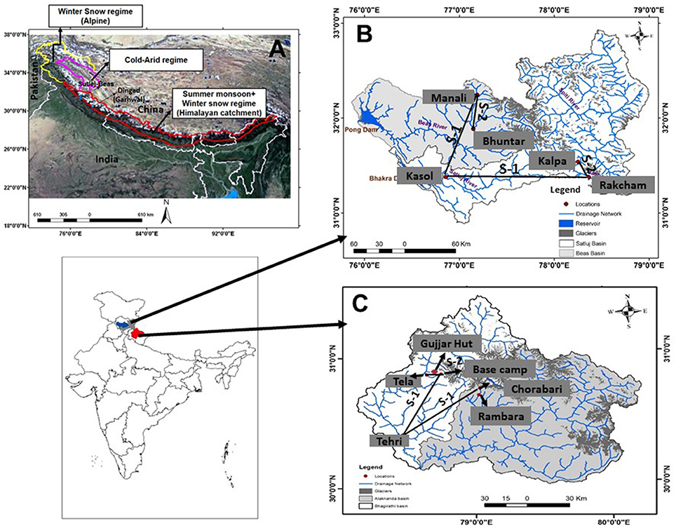
Figure 1. (A) Glacio-hydrological regimes of southern slopes of the Himalaya and study area (after Thayyen and Gergan, 2010) and study basins in the monsoon regime: (B) Sutlej and Beas basins (C) Bhagirathi and Alakanada basins in the upper Ganga basin.
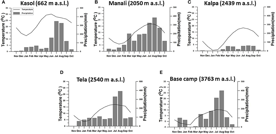
Figure 2. Monthly distribution of temperature and precipitation at different elevations of the study basins. Sutlej–Beas basin (A–C) and upper Ganga basin (D,E).
Methodology
In the present work, we analyse the SELR of temperature using data from three stations in the Sutlej basin, two stations in the Beas basin and five stations in the upper Ganga basin. Mean daily temperature and precipitation data of Beas and Sutlej basins were sourced from Bhakra Beas Management Board (BBMB). Data of Kasol (662 m a.s.l.), Bhuntar (1,089 m a.s.l.), Manali (2,050 m a.s.l.), Kalpa (2,439 m a.s.l.), and Rakcham (3,130 m a.s.l.) were used in the study. Kasol, Kalpa, and Rakcham data of 1986–2007 and Manali–Bhuntar data of 1986–2000 were used to study the temporal and inter-annual changes in the temperature lapse rate. For upper Ganga basin, data collected from Dingad catchment at three stations located at Tela (2,540 m a.s.l.), Gujjarhut (3,483 m a.s.l.), and Basecamp (3,763 m a.s.l.) (Figure 2B) under two separate sponsored projects under the Indian Himalayan glaciology programme of the Department of Science and Technology (DST), Govt. of India during 1998–2004 period are being used. Temperature data of Tehri (770 m a.s.l.) is sourced from Central Research Institute for Dryland Agriculture (CRIDA) for 2000–2007 period. SELR data between Rambara (2,760 m a.s.l.) and Chorabari (3,820 m a.s.l.) and mean monthly temperature data of Chorabari (2011–12) in the Alakanada basin is sourced from published literature (Kesarwani et al., 2012; Kesarwani, 2016).
All thermometers used in the manual measurement stations were factory calibrated as per the India Meteorological Department (IMD) standards and the final data were prepared by applying correction factors to the raw data. During the period of manual measurements, mean daily humidity was calculated from mean daily saturated and actual vapor pressures data were measured from dry bulb and wet bulb temperatures. Mean daily specific humidity was estimated by deriving mean daily actual vapor pressure from mean daily humidity (see Annexure for detailed methods). Temperature measurements were taken using calibrated thermometers and identical passive ventilation shields were used for stations in each region. Hence, relative observational errors between the stations in each region are expected to be minimal. In addition, SELR is calculated as a difference of temperature between two elevation points and hence influence of marginal measurement errors gets minimized further in this analysis.
Deriving reliable precipitation information over the high altitude regions of the Himalaya, especially measuring snowfall is a big challenge (Ménégoz et al., 2013; Shrestha et al., 2014). Hence, precipitation data are used only for describing the regional climatology. Solid precipitation collected in the standard rain gauges was measured as water equivalent after melting as per the IMD standard procedure. Further, standing snow depth and density were monitored four times during the December–April period at different altitudes along the valley bottom from Gujjar Hut to the Basecamp and accumulated snow water equivalent was calculated (Thayyen and Gergan, 2010). Many of these surveys conducted immediately after the snowfall events have shown that the precipitation measured by the rain gauge underestimates it by 26–32%. A study conducted in Nepal using tipping bucket rain gauge and differential change in the snow depth showed around 60% under reporting by the rain gauge (Shrestha et al., 2012). Here, monthly total precipitation values were arrived at by adding 30% to the precipitation measured by rain gauge during the peak snowfall season.
The average temperature decrease with height in the free atmosphere is generally called “environmental lapse rate” (Barry, 2008), which usually approximates between 6 and 6.5 K/km. The temperature lapse rate along the mountain slopes significantly differs from the free atmosphere or environmental lapse rate (Marshall et al., 2007; Minder et al., 2010; Heynen et al., 2016). This temperature lapse rate along a mountain slope is termed here as the Slope Environmental Lapse Rate (SELR). The SELR variation is driven by naturally occurring orographic factors whereas environmental lapse rate of the free atmosphere is driven by vertical displacement of the air parcel. SELR between a pair of stations is calculated by the equation,
Where T1 and T2 are the mean monthly temperature of lower and upper stations, respectively, in Kelvin, and H1 and H2 are the elevations of the lower and upper stations in kilometers. SELR is calculated for different altitude sections in the Sutlej, Beas, and upper Ganga basin to understand elevation dependency of the slope lapse rate values of temperature vis-a-vis the moisture regimes. The pair of stations constrained in the high elevation nival–glacier regime is termed as section 2 and other pairs representing the basin scale and valley scale SELR response is termed as section 1 (Figure 1). In the upper Ganga basin four pairs under section 1 are discussed. They are 1. Tehri (770 m a.s.l.)–Basecamp (3,763 m a.s.l.), 2. Tehri–Chorabari (3,820 m a.s.l.), 3. Tela (2,540 m a.s.l.)–Basecamp, and 4. Rambara (2,760 m a.s.l)–Chorabari. Section 2 in the upper Ganga basin is represented by Gujjarhut (3,483 m a.s.l.)–Basecamp (3,763 m a.s.l.) station pair. Similarly, in the Sutlej–Beas basin section 1 is represented by Kasol 662 m a.s.l.–Rakcham, 3,130 m a.s.l. and Kasol–Manali (2,050 m a.s.l.) station pairs. Kalpa (2,439 m a.s.l.) and Rakcham (3,130 m a.s.l.) stations are paired for representing the nival–glacier regime (section 2) of Sutlej basin and Bhuntar (1,089 m a.s.l.) and Manali (2,050 m a.s.l.) stations pair for Beas basin. In the following discussions, these sections will be referred as defined above. The present study is based on the mean monthly SELR derived from mean monthly temperature of the stations described above.
Lifting condensation level (LCL) is calculated to explore its relationship with the SELR using the relationship LCL(m) ~ 125 (T – T_d). Where T and Td are temperature and dew point temperature at the near surface. This relationship is accurate within about ±2% for 50% ≤ RH ≤ 100% and 0° < T < 30°C (Lawrence, 2005).
Modeling SELR for Monsoon Regime
The environmental lapse rate of 6.5 K/km is the linear lapse rate of the troposphere considered as one single layer in the U.S. standard atmosphere (NOAA, 1976). The equations governing the Dry Adiabatic Lapse Rate (DALR) and Saturated Adiabatic Lapse Rate (SALR) are well-established. However, these equations are generally used in the context of air parcels lifted “vertically” upwards under different moisture conditions. Though various studies pertaining to lapse rate over other mountainous regions prevail (Thyer, 1985; Rolland, 2003; Harlow et al., 2004; Blandford et al., 2008; Minder et al., 2010) a model which encapsulates the mountain process remains a challenge. Over central Himalaya, Kattel et al. (2013) has provided lapse rate estimation with functional reference of the elevation. Here, we are proposing a simple solution to capture the seasonal SELR variations observed in the monsoon regime with a hypothesis that the moisture influx during the monsoons and lack of it during the rest of the period, especially during April, May, and June (AMJ) is a major factor responsible for the seasonal variations in the LCL in an orographic system which in turn play a decisive role in determining the valley scale SELR and temperature distribution along the valley slopes as discussed in section 5 below.
The DALR and SALR of the free atmosphere is governed by the following equations respectively (Robinson and Henderson-Sellers, 1992),
where, dt/dz is rate of change of temperature (T, Kelvin) with height (z), g is acceleration due to gravity (9.8 m/s2), Cp is specific heat at constant pressure (1.004 J/g-K), L is the latent heat of phase change (L = 3,071 – 2.134 T J/g), ws is the saturation mixing ratio.
where es is saturation vapor pressure and p is the mean station pressure in hPa.
To solve this equation, temperature data at two elevations are required for estimating the change in the saturation mixing ratio. This equation provides valuable insight into processes governing the temperature lapse rate under saturated conditions, but failed to represent the SELR of the region (Figure 3). This equation also does not have the predictive advantage as it requires temperature from a lower and upper station. What is required for the Himalayan region is a SELR model for estimating the higher elevation temperature based on the temperature data at the lower elevation station. The following relationship of pseudo adiabatic lapse rate (Equation 4) is found to be appropriate for this purpose (Peixoto and Oort, 1992).
where
where, T is the base station temperature in Kelvin, P is mean base station pressure in hPa,ε is the ratio between molecular weight of the water vapor and apparent average molecular weight of dry air gases (0.622), and R is gas constant for dry atmosphere (0.287 J g−1 K−1). There are different forms of this equation available in the literature. We chose this equation due to its explicit reference to the elevation (pressure) of the temperature measurement station. Equation (4) shows significant improvement over Equation (2) (Figure 3) but the difference between modeled and observed SELR is still found to be very significant and devoid of observed seasonal variations characterizing the pre-monsoon and monsoon regime.
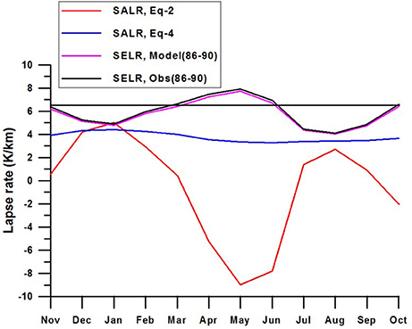
Figure 3. Temperature lapse rate of section 1 of Beas basin between (Kasol, 662 m a.s.l. and Manali, 2,050 m a.s.l.) calculated by using the Equation (2) and Equation (4) showing significant deviation from the observed SELR highlighting the need for a new approach. Modeled SELR of the section using derived indices shows promising result. Monthly average temperature of 5 years (1986–1990) was used here to develop the monthly indices for the model.
To improve the response of Equation (4), the fraction of moisture (dwsf) potentially responsible for forcing the observed SELR has been calculated using the observed SELR and estimated SALR using Equation (2) as described below:
where, dwsf represents the potential withdrawal/influx of moisture within the elevation section with reference to the respective SALR.
By using this information, we have derived monthly SELR indices (Mi) for section 1 of the monsoon region as follows for “n” number of years:
These monthly indices are applied to the Equation (5) and modified “N” has been calculated as shown in the Equation (8) below. Eventually this newly derived “N” is applied to the Equation (4) to derive the SELR for different sections under different basins of the monsoon regime.
SELR modeling is attempted only for valley scale lapse rate (section 1) which have higher inter-annual stability as compared to the lapse rate of nival–glacier system (section 2) as discussed in the section SELR Variations in the Nival–Glacier Regime below. Monthly SELR indices calculated for the section 1 (Kasol–Manali) for a period of 1986–1990 and used for testing the applicability of the SELR model for section 1 of all the three basins (Beas, Sutlej, and upper Ganga basin) for different time periods. The 10 year mean monthly SELR of the Sutlej and Beas basin (1991–2000) and the mean monthly SELR for 5 individual years were tested and it was demonstrated that the indices derived at one section are suitable across the region under the study. The indices were further refined by K-fold cross validation (K = 5) using all the data of 1986–2005 period of Sutlej–Beas basins and regional monthly indices were developed. These regional indices were further tested for 2006 and 2007 mean monthly temperature data from Kasol–Rakcham section as well as for the Tehri–Basecamp, Tehri–Chorabari, and Tela–Basecamp sections in the upper Ganga basin for demonstrating its regional validity. The model further tested for deriving the daily SELR of selected sections in the Sutlej and upper Ganga basin depending on the data availability. Performance of the model has been tested by calculating the Root Mean Square Error (RMSE) and p-value. Model results were further evaluated with standard environmental lapse rate of 6.5 K/km for assessing the improvement achieved through the proposed solution.
Results
Valley Scale SELR Variations
Seasonal variations in the valley scale SELR (section 1) of all the three basins under the monsoon regime (Sutlej, Beas, and upper Ganga basins) of the western Himalaya have shown remarkable similarity and closely followed the characteristics of the near surface temperature lapse rate of the Nepal Himalaya (Kattel et al., 2013; Immerzeel et al., 2014). Lowest SELR was recorded during monsoon months of July and August and highest SELR was observed during April and May months. SELR of winter months was also significantly lower than that of April and May months in all the basins (Figure 4). Annual range of mean monthly SELR is significant in all the three basins extending from 4.1 to 8.1 K/km for the Kasol–Manali section and 5.0–7.6 K/km for the Kasol–Rakcham section in the Sutlej–Beas basin. In the Ganga basin, it varies between 4.9 and 7.1 K/km for the Tela–Basecamp section, 3.6 and 6.1 K/km for the Tehri–Basecamp section, and 4.5 and 7.4 K/km for the Tehri–Chorabari section (Table 1). Long-term mean SELR (1986–2000) of the Kasol–Manali sections during monsoon months of July and August were 4.4 and 4.1 K/km, respectively. For the Kasol–Rakcham section it stands at 5.0 K/km for both the months. In the Ganga basin July, August SELR range between 4.6 and 5.1 K/km for the Tehri–Basecamp, 4.9 and 5.0 K/km for the Tehri–Chorabari, and 5.3 and 5.4 K/km for the Tela–Basecamp sections. This monsoon lowering is similar to that reported from Nepal region including that of Everest region (Salerno et al., 2015). Rambara–Chorabri section recorded the lowest July, August SELR of 3.6 and 3.3, respectively, for section 1. This clearly suggests that the monsoon lowering of SELR is a regional phenomena covering upper Ganga and Sutlej–Beas basins of the western Himalaya as well as Nepal Himalaya as reported earlier (Kattel et al., 2013; Immerzeel et al., 2014). Monsoon transition month of September continues to experience predominantly lower lapse rate and the post-monsoon month of October experiences predominantly higher (>5.8° K/km) SELR. We also looked into the inter-annual variability of valley scale SELR of the Kasol–Manali and the Kasol–Rakcham sections using 15–20 years of available data. The coefficient of variation of SELR for valley scale SELR ranges from 0.06 to 0.17, which suggests a high inter-annual stability of valley scale SELR (Figure 5).
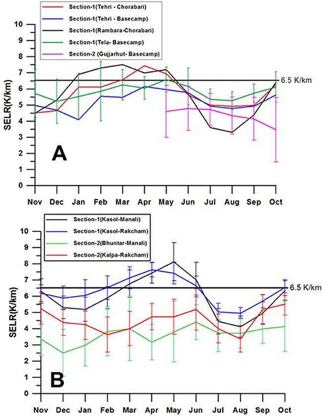
Figure 4. Monthly SELR variations of section 1 and section 2 in the monsoon regime (A) Upper Ganga basin and (B) Sultej and Beas basins. Standard deviation in the data is also shown.

Table 1. Slope Environmental Lapse rate (SELR) of temperature in the monsoon regime of western Himalaya along nine profiles covering Sutlej, Beas, and upper Ganga basins.
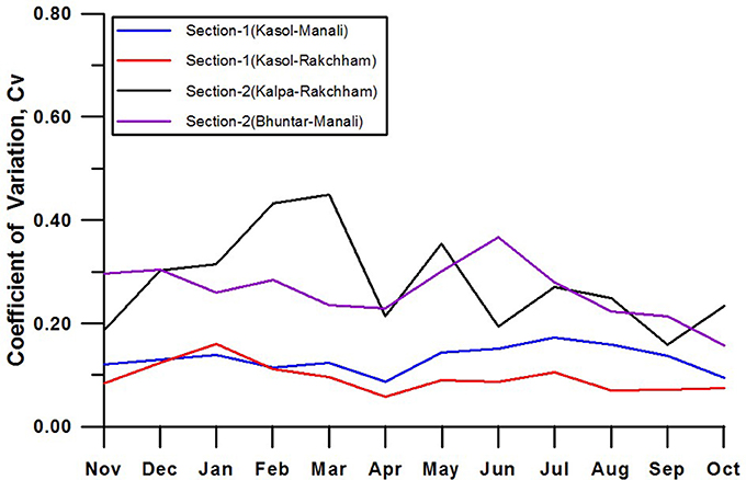
Figure 5. Coefficient of variation (Cv) of section 1 and section 2 of Sutlej and Beas basins showing higher inter-annual stability of valley scale SELR(section 1) as compared to nival–glacier regime SELR (section 2) during 1986–2000/2007 period.
SELR Variations in the Nival–Glacier Regime
SELR of section 2 representing the nival–glacier regime (Figure 1) is considered important for cryospheric system studies in the Himalaya. Generally, studies on Himalayan glaciers focus on the data collection of glacier regime following the benchmark glacier monitoring strategy which includes weather monitoring very close to the glaciers (Fountain et al., 1997). This station data is extrapolated to the higher elevations using standard temperature lapse rates for glacier wide studies. It is also well-known that the monsoon precipitation declines as we move up the higher elevations (Bookhagen and Burbank, 2010). Therefore, characteristics of the SELR response constrained within these elevation zones acquire significance. It can be seen that the SELR of nival–glacier regime (section 2) of all the three basins are significantly different from the SELR of valley scale SELR. Section 2 is characterized by lower SELR across the seasons (Figure 4). Absence of significant intra-seasonal SELR variation is also noted as a key difference as compared to section 1. Due to this, “monsoon lowering” of valley scale SELR is absent from section 2 of Beas and Dingad basins. However, section 2 of the Sutlej basin does experience subdued monsoon lowering. Long-term (1986–2000) monthly mean SELR of section 2 of Beas basin (Bhuntar–Manali) vary between 4.4 and 2.5 K/km and that of Kalpa–Rakcham (1986–07) vary between 5.5 and 3.4 K/km. For Dingad catchment, section 2 data are available only for summer months (MJJASO) and varies between 2.1 and 4.6 K/km with few exceptions. One major observation regarding the SELR of the nival–glacier regime is its weak inter-annual stability. Coefficient of variation of section 2 SELR is found to be greater than section 1 throughout the year (Figure 5) and varies between 0.46 and 0.16. With lack of supporting data from these stations, possible factors driving these inter-annual changes could not be ascertained. This result highlights the need for significant further research to build data and concepts for a comphrehensive atmospheric model valid across the elevation ranges of the Himalaya.
SELR and Specific/Relative Humidity Relationship
The amount of water vapor in the atmosphere and its seasonal variations could be playing an important role in forcing the SELR variations. Some insights on these aspects are developed from the data generated from Dingad catchment. Higher specific humidity during monsoon months of July and August is characteristic of this regime. Mean monthly specific humidity at 2,540 m a.s.l. varies between 3.59 and 16.4 g/kg during the observation period. Highest observed value of specific humidity was 18.17 g/kg in the month of July 1998. At higher elevation (3,763 m a.s.l.) mean monthly specific humidity ranges between 2.92 and 11.4 g/kg. It is noted that the water vapor in the atmosphere during winter months (NDJFM) ranges from 2.92 to 5.3 g/kg and is significantly lower than the monsoon period (Figure 6). It is observed that the higher elevation stations generally experience lower specific humidity throughout the year. Feld et al. (2013) also observed a similar response in the Sierra Nevada Mountains in California. Monthly mean relative humidity of the uppermost station in the monsoon regime (3,763 m a.s.l.) remained above 80% during the peak monsoon months leading to sustained lower SELR of section 2 during these months, while relative humidity at the lower station (2,540 m a.s.l.) fluctuates between 65 and 80% during the same period. Low relative humidity and corresponding higher LCL in April and May result in higher SELR and higher relative humidity and lower LCL in monsoon months result in lower SELR as explained in the section 5 below.
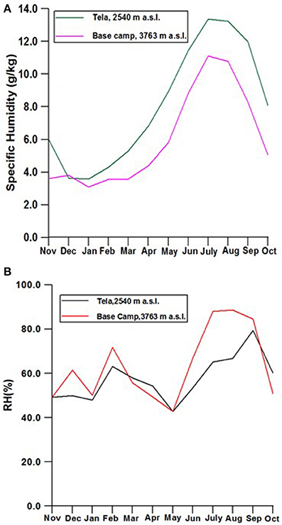
Figure 6. Mean monthly specific humidity variations of (A) lower (2,540 m a.s.l.) and upper (3,763 m a.s.l.) stations of Dingad catchment and (B) corresponding seasonal variations in relative humidity.
Modeling Results of Valley Scale SELR
Standard lapse rate equations as described in Equations (2) and (4) were implemented to test their response along sections 1 of Beas basin (Kasol–Manali) using mean monthly temperature and SELR of 1986–90 period. Seasonal variability is more pronounced for Equation (2) as it uses the estimate of change in saturation mixing ratio between the two stations for calculating the heat generated due to condensation process. On the contrary, Equation (4) is more stable as it uses saturation vapor pressure value of single station for calculating the potential heat generated during condensation (Figure 3). Both the models are in better agreement with the observed SELR in winter (DJ) and monsoon months (JA). April, May, and June months experienced highest deviation between observed SELR and calculated SALR. It is noted that the observed SELR values were higher than the calculated SALR values for the section 1. These deviations are resolved by developing SELR indices as suggested by Equation (7). Developed indices for the Kasol (662 m a.s.l)–Manali (2,050 m a.s.l.) section for 1986–90 period are given in Table 2. Derived monthly indices were tested in the same section by using decadal mean monthly temperature of Kasol (662 m a.s.l.) for 1991–2000 period. The model performance is found to be good with a p-value of 5.81 × 10⁻⁹ and an RMSE of 0.35 K/km
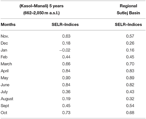
Table 2. Comparison between monthly SELR indices (Mi) derived from Kasol (662 m a.s.l.) to Manali (2050 m a.s.l.) section using monthly mean temperature data of 1986–1990 period and regional indices derived through 5-fold cross validation of Kasol–Manali and Kasol–Rakcham data 1986–2000/2005 period.
(Table 3). Further, the model is tested for five individual years from 1996 to 2000, with p-value ranging from 1.77 × 10⁻⁴ to 9.89 × 10⁻³ and RMSE from 0.70 to 1.17 K/km. To assess the regional validity of the derived indices, the model is tested for section 1 of the Sutlej basin (Kasol–Rakcham). Testing was undertaken with decadal mean monthly temperature and SELR (1991–2000) as well as for individual years from 2003 to 2007. Model has performed well with p-value ranging from 1.0 × 10⁻⁵ to 4.3 × 10⁻³ and RMSE ranging from 0.43 to 0.85 K/km. Further, the indices were tested for the upper Ganga basin for 2 full years (2002–03 and 2003–2004) and 4 years of summer ablation months (May–October). Results support the applicability of the indices developed in the Beas basin for upper Ganga region as well with p-value of 1.09 × 10⁻⁴ to 3.91 × 10⁻³. However, significantly higher RMSE values ranging from 1.09 to 1.23 K/km were noted for this section. This suggests the need for refining the indices developed using small set of data of one section alone. In general, this exercise has established the applicability of the model across the study region under the influence of monsoons and for different time periods.
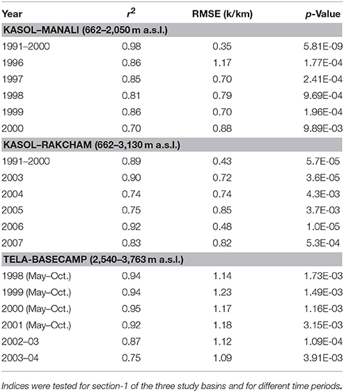
Table 3. Details of error analysis from the preliminary test of the 5-year mean (1986–1990) SELR indices of Kasol–Manali section.
The regional performance of the model has been further improved by K-fold cross validation utilizing all the available mean monthly temperature data of Sutlej–Beas basin from 1986 to 2005 period. In K-fold cross validation all the available data is partitioned into K equally sized sections and an iterative training and validation are performed by using K-1 folds for learning in each iterations and validated using the one held-out fold. The monthly indices were refined by five-fold cross validation of both the sections in the basin. The cross validation statistics are presented in the Table 4, which suggested consistent response of the model across the folds. Regional monthly indices are derived through this exercise by averaging the results (Table 2). These indices are tested with each test fold data as well as with two years of new data from Kasol–Rakcham section and for three sections in the upper Ganga basin. The regional indices have shown better performance across the study sections (Figure 7). The relative error for monthly SELR various folds of the Kasol–Manali and the Kasol–Rakcham sections ranges between 4.3 and 8.6%. For the Tela–Basecamp section, the model has shown significant improvement in RMSE in the range of 0.53 to 0.67 from 1.09 to 1.23 from the preliminary test (Table 5) with relative error in the range of 8.2–9.8%. Model also tested effectively in the Kasol–Rakcham section for 2006 and 2007 data with an RMSE of 0.53 and 0.50 and relative error of 7.2 and 7.4% respectively. The Tehri–Basecamp section and Tehri–Chorabari section showed significantly higher relative error of 15 and 13.4%, respectively. The performance of the model was further tested with the standard Environmental lapse rate of 6.5 K/Km which returned significantly higher RMSE across the study sections in the range of 1.17–0.91 as compared to the model vs. observation RMSE of 0.84–0.33. This clearly indicates the significant advantage of using the proposed model over the standard environment lapse rate in the monsoon region on a monthly scale.
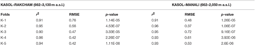
Table 4. K-fold cross validation statistics of the Kasol–Manali and Kasol–Rakcham sections.
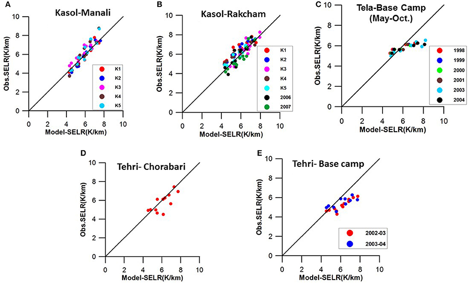
Figure 7. Relationship between modeled and observed SELR using regional indices derived by K-fold cross validation. Regional indices were tested against each test folds of Kasol–Manali (A) and Kasol–Rakcham (B) sections as well as for the new data set of 2006 and 2007. Regional indices were further tested for different profiles of the upper Ganga basin (C–E) showing the significant improvement achieved through cross validation and its regional validity.
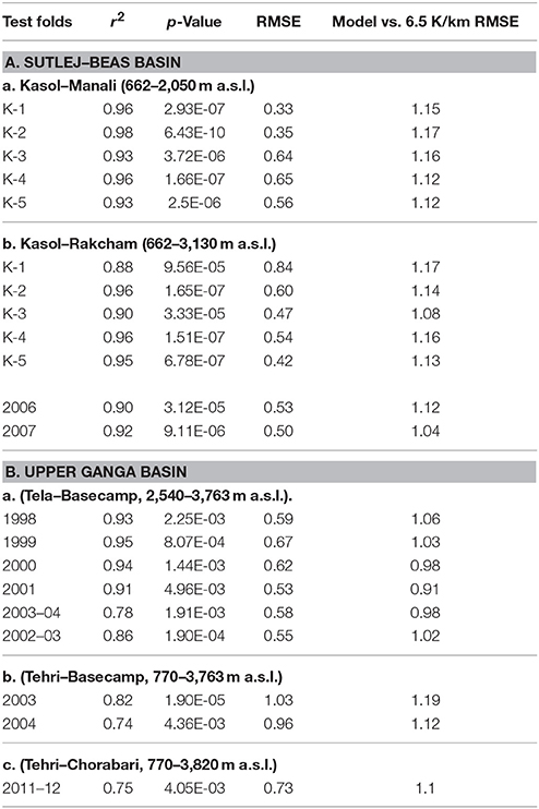
Table 5. Model test statistics using regional monthly SELR indices and mean monthly temperature for (A) Sutlej–Beas basin data (a) Kasol–Manali (662–2,050 m a.s.l.) and (b) Kasol–Rakcham (6,62–3,130 m a.s.l.) sections and (B) for upper Ganga basin; (a).Tela–Basecamp (2,540–3,763 m a.s.l.), (b) Tehri–Basecamp (7,70–3,763 m a.s.l) and (c) Tehri–Chorabari (770–3,820 m a.s.l) Significant improvement in the model performance using regional indices over the 5 year indices derived for Kasol–Manali section is observed. Model performance against the standard environmental lapse rate (6.5 K/km) is significantly poor as compared with the observations indicating the improvement achieved through the modeling efforts.
Regional mean monthly SELR indices were further tested for daily SELR estimation in the three study basins for selected years based on the daily data availability. It is found that the higher elevation stations have number of missing data either of maximum or minimum temperature, especially for the Manali station. Daily SELR is tested for the Kasol–Rakcham section during 2000–2007 period. The results show lower correlation and higher RMSE ranging between 1.0 and 1.4 K/km as compared to the monthly model results and the relative error ranges between 14.3 and 18.4%. However, the p-value shows significant improvement for daily model results. The daily SELR modeling of the Kasol–Manali section is carried out for 1986–88 and 1998–2000 periods and the relative error ranges from 17.4 to 22% In the Ganga basin, daily SELR modeling were carried for the Tehri–Basecamp and the Tela–Basecamp sections for 2 years during 2002–03 and 2003–04. All these sections show similar results in terms of correlation, RMSE and p-value (Figures 8A–C and Table 6). Average relative error of the Ganga basin section was 19.2%. The modeled daily SELR matches well with the temporal averages of observed SELR and run through the mean of the daily SELR fluctuations (Figure 8D). On a daily basis, the model error accounted for 14.3–22%, which suggests that even with the mean monthly SELR indices, 78–80% of the daily SELR variations are accounted by the proposed modeling solution which further improved to more than 90% for monthly analysis. Hence, it can be considered that the daily residuals are forced by the daily LCL variations and other local factors. The results of monthly and daily SELR modeling are promising while considering the large number of possible factors influencing temperature lapse rates along the mountain slopes (Marshall et al., 2007) as well as the limitations associated with the data and knowledge in the Himalayan region. Further improvement to the proposed model could be achieved by developing appropriate data and methods to link daily LCL variations and associated dynamics with other local land surface processes.
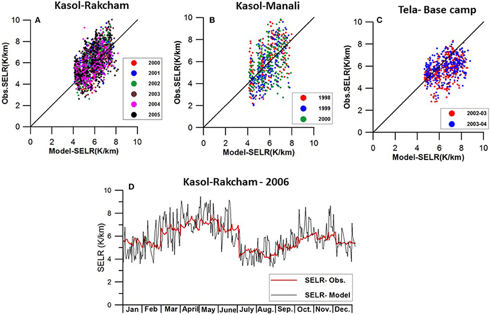
Figure 8. Testing of monthly SELR indices for daily lapse rate assessment of (A) Kasol–Rakcham and (B) Kasol–Manali section in the Sutlej–Beas basin and for (C) Tela–Basecamp section in the upper Ganga basin. Model has been sucessful in estimating the temporal mean lapse rates but not suceeded in capturing the day to day SELR variations (D).
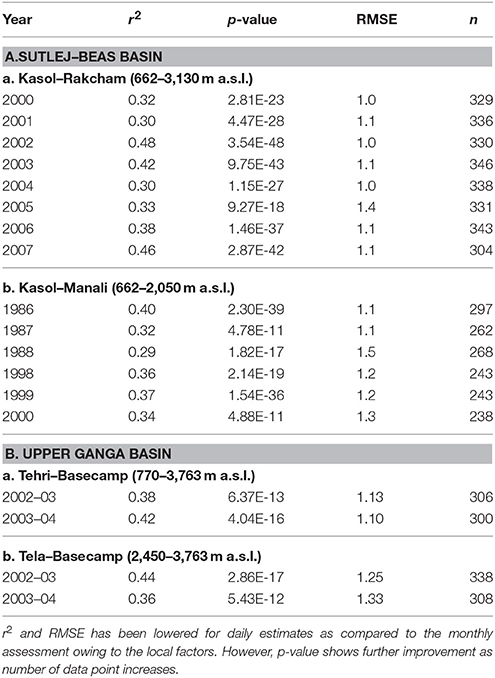
Table 6. Results of the model test for daily SELR for (A) Sutlej–Beas basin data (2000–2007) (B) For upper Ganga basin.
Discussion
Seasonal variations of valley scale SELR observed for Beas, Sutlej and upper Ganga basins in the present study is comparable with the observations reported from Neaplease Himalaya (Kattel et al., 2013; Heynen et al., 2016) and suggest that the processes controlling the SELR are similar across the monsoon regime of the central and western Himalayan region. Long-term consistency of seasonal responses as shown in the present study also underlines this aspect. SELR lowering during the key monsoon months and higher valley scale SELR during April, May, and June months has emerged as the key characteristics of the “Himalayan catchment” dominated by the monsoons. Significantly lower SELR of the nival–glacier regime (section 2) comparable to the SALR persisting across the seasons is another important characteristic identified for the first time. Seasonal variations in the influx of moisture into the “Himalayan catchments,” its orographic lifting, corresponding LCL variations and resultant latent heat release during condensation could be guiding these responses. Significant proximity of SELR of section 1 with that of the theoretical SALR for corresponding pressure levels during the ISM months is indicative of this process (Figure 9). Dominance of the large scale circulation over local slope and valley winds on temperature lapse rate is reported from Alps also (Kirchner et al., 2013). Lower mean monthly SELR of nival–glacier regime (section 2) equaling plausible SALR for corresponding pressure levels throughout the year (Figure 9) is another clear indication of the role of the orographic lifting of the air mass in regulating the SELR and forcing the deviation from the standard environmental lapse rate of 6.5 K/km. Higher inter-annual variability of SELR in the nival–glacier regime as observed for Beas and Sutlej basins is indicative of the influence of more complex local processes driving these changes in the upper reaches. This raises questions regarding its use for modeling snow and glacier melt, especially for modeling future runoff and glacier fluctuations. Various researchers have shown that the glacier and snowmelt estimation by degree day method is highly sensitive to the near surface temperature lapse rates (Marshall et al., 2007; Gardner and Sharp, 2009; Immerzeel et al., 2014). This result points toward the need for re-visiting the benchmark glacier monitoring strategy (Fountain et al., 1997) for mountain glaciers. Under this strategy, climate monitoring for glaciological studies are focused on the glacier regime, which limits our ability to understand/incorporate key orographic processes at lower elevations forcing the temperature variations at the higher elevations. The results suggest that the use of valley scale SELR having higher inter-annual stability may be more appropriate for extrapolating the temperature to the higher elevations until the challenging task of development of a full atmospheric model which encapsulate the various local processes over a complex terrain driving the SELR across the mountain elevations takes place.
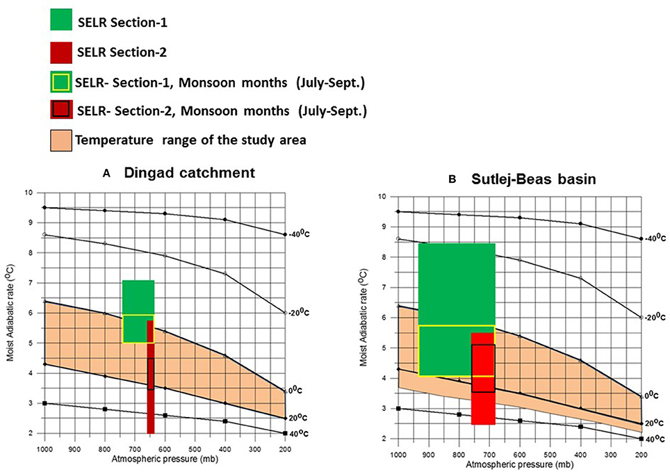
Figure 9. Theoretical saturated adiabatic lapse rate (SALR) under different pressure–temperature combinations calculated using Equation (4) and observed monthly SELR under monsoon regime (A) Dingad catchment and (B) Sutlej–Beas basin. Green blocks showing the extent of mean monthly SELR of section 1 and Red blocks for section 2. Yellow outline represents the SELR range of section 1 during the monsoon months and blue outlines for section 2. Both fall within the theoretical SALR range suggesting the influence of moisture influx and related monsoon lowering of SELR. Higher SELR of April, May, and June months is also common to all the study basins.
Observed seasonal SELR variations in the study region range from 8.1 to 2.5 K/km which deviate significantly from the standard environmental lapse rate. This difference could be forced by the orographic lifting of the air mass along the mountain slopes. In the case of displacement of air parcel along a vertical air column, such variations in the lapse rate occur above and below the LCL (Ahrens, 1991). Analysis in the Sutlej and Dingad catchment suggests that the same processes are followed by the air parcel while being lifted along the mountain slopes by the orography as well. Significant correlation between LCL at 2,540 m a.s.l. and SELR of section 1 (r2, 0.59–0.72, P < 0.001) in the monsoon regime during the observation years suggest that the seasonal LCL height variation plays a dominant role in determining the SELR, especially in the pre-monsoon and monsoon periods. In both the basins, LCL in summer/monsoon months is found to be closer to the land surface, forcing SELR toward SALR (Figure 10). On the contrary, LCL shifts to the higher altitudes during moisture deficit months of April, May and June in the pre-monsoon period forcing higher SELR for section 1 shifting toward the DALR in all the three basins under study (Figure 10). A major process consuming significant energy within the parcel is the re-evaporation of condensed precipitation while falling through the warmer layers below (Dolezel, 1944). We propose that the rate of re-evaporation of water droplet, governed by the seasonal variations in the LCL could be playing an important role in determining the seasonal variations in the valley scale (section 1) SELR. This process has been incorporated in the proposed model through the monthly SELR indices and explains why similar seasonal SELR responses exist across the study region. It can be seen that the monthly variations in the SELR indices closely follow that of LCL variations with higher LCL forcing higher monthly SELR index. This implies that a significant portion of the latent heat released at the higher altitude region during March, April, May, and June months is consumed for re-evaporation and forcing the lapse rate along the mountain slopes to the higher side. While during the monsoon months, orographic lifting of the incoming moisture forces LCL closer to the mountain slopes and most of the latent heat released is available for warming the region and reducing the temperature gradient. The same pattern is also reflected in the relative humidity (RH) variations with lower RH during March, April, May, and June as compared to July and August. The amount of water vapor in the atmosphere during winter months is significantly less than the summer months and higher elevations have less water vapor as compared to the lower elevation stations (Figure 6A). However, lower temperatures ensure lower LCL during this period. We suggest that the higher LCL and higher valley scale SELR during April, May, and June months is very critical for higher elevation cryospheric region as it contributes to the shift in the warmest months from May to June at the lower elevations to July to August at the higher elevations. SELR variations could also be influenced by factors such as land surface conditions (Pepin and Losleben, 2002; Pepin and Kidd, 2006). However, Kirchner et al. (2013) found no significance difference between snow and no snow cover days in lapse rate based on daily mean temperature. The present study considered moisture dynamics in an orographic system by linking LCL and SELR and the reported RMSE of the model results suggest that around 90% variability of monthly SELR and 80% variability of daily SELR is explained by the monthly mean indices. This also suggests that the surface conditions and other local processes such as cold air pooling and differences in net radiation have more influence on the daily SELR. The present study establishes a major process driving the valley scale slope lapse rate of the monsoon region of the Himalaya.
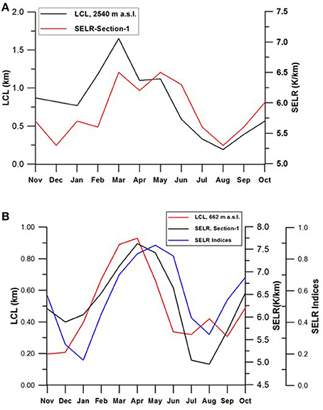
Figure 10. Seasonal variations of valley scale SELR is closely linked to the LCL variations in the monsoon region. Both (A) Upper Ganga basin and (B) Sutlej/Beas basin show similar response suggesting it as a regional characteristic influencing the valley scale SELR. Derived regional SELR indices are closely linked to the seasonal variations in LCL confirming this linkage.
Comparison With Free Environment Temperature Lapse Rate of the Study Areas
We have seen that the seasonal SELR variations have regional characteristics and are linked with the seasonal moisture conditions as well as seasonal variations in the regional LCL. Therefore, we further studied how the lapse rates derived from reanalysis and climate model compares with the observed SELR. Environmental lapse rate of the free atmosphere is calculated from the ERA–interim reanalysis (Dee et al., 2011) (https://apps.ecmwf.int/auth/login/), and regional climate model (RCM) from the Max Planck Institute for Meteorology (REMO) (Jacob et al., 2007). “The ERA–Interim reanalysis is produced with a sequential data assimilation scheme, advancing forward in time using 12-hourly analysis cycles. In each cycle, available observations are combined with prior information from a forecast model to estimate the evolving state of the global atmosphere and its underlying surface” (Dee et al., 2011). REMO model simulation uses global ERA–interim reanalysis data to supply large-scale boundary information. The RCM inputs will be important information for providing finer scale regional climate accounting for regional feedbacks, physical processes and dynamical forcing. ERA–Interim and model details are not provided here as it is not the core focus of this paper. Discussion is limited to the comparison with corresponding initial and boundary conditions from ERA–interim and corresponding station observations. It is important to mention here that various reanalysis are amalgamations of observed station records, and satellite information, and uses different mathematical and statistical algorithms to generate the reanalysis data. These are also not discussed here in detail as it is out of the scope of the present work. However, better quality of the ERA–interim data over other reanalysis data is proven as it uses observed surface temperature records during its preparation (Simmons et al., 2004, 2010). This particular fact is very important for the Himalayan region due to paucity of the observation network and may give a benchmark for future research in the absence of such records. Corresponding ERA–interim forcing to simulate the REMO regional climate model is expected to provide more exhaustive information over the study region. Hence, ERA–interim data records for the period 1998–2004 for monsoon regime at Tela (30°51′26.22″N, 78°40′39.96″E) and Sutlej/Beas (31°15′-33°0′N, 77°30′-79°0′E) for 2000–2007 period are extracted to compare with the corresponding station observations. Observed and ERA–interim environmental lapse rate matches well with summer monsoon lowering for valley scale SELR for the study basins (Figure 11). For Dingad catchment, November to April period shows significant difference between the two; whereas for Sutlej/Beas basin, more difference is observed during April to June. It is observed that the ERA–Interim give same lapse rate for different altitude sections and fails to capture the unique SELR response of the nival–glacier section (section 2). Environmental lapse rate derived from REMO follows the same trend of ERA–interim but with higher values for upper Ganga basin. Hence, REMO has not been tested for Sutlej/ Beas basin. Whiteman and Hoch (2014) showed that the relationship between the pseudo-vertical temperature and radiosondes improves with elevation and steepness of the slope. It is important to mention here that ERA–interim is at 1° × 1° lat/lon horizontal resolution, which is too coarse over the region of study with heterogeneous land use and variable topography. Fiddes and Gruber (2014) have extensively shown the downscaling method of climate variables from coarser to finer resolution over heterogeneous topographic regions. It could be inherent that during the preparation of the reanalysis, most of the sub-grid scale processes are not being captured within the resolution of reanalysis. However, it is obvious that environmental lapse rate based on ERA–interim and REMO are sensitive to moisture. It is evident that both ERA interim and REMO gives comparable temperature lapse rate during the monsoon months. This study suggests that the gridded reanalysis data captures some key regional processes such as monsoon lowering of valley scale SELR but fails to capture pre-monsoon response of higher SELR as well as lower SELR of nival–glacier regime (Figures 11A,B). For downscaling near surface temperatures, SALR of 6–7 K/km is generally used (Flowers and Clarke, 2002; Bassford et al., 2006; Raper and Braithwaite, 2006). This suggests that the improvement is needed on this front as well and development of a full atmospheric model integrated with the processes described in this paper and other land surface processes of the mountain slopes are essential to capture the observed SELR variations shown in the present study. Gerlitz (2015) showed how ERA–Interim reanalysis data over a complex central Himalayan terrain can be used for estimating near surface temperatures by coupling it with a fuzzified regression tree model with local terrain parameters as potential predictors. Considering the limitations of ERA–Interim reanalysis described above, such methods could be further improved by the proposed approach in this paper.
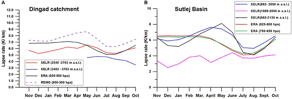
Figure 11. Comparison of ERA–interim free environment lapse rate with SELR of (A) Dingad catchment and (B) Sutlej–Beas basin. Free Environment lapse rate derived from REMO RCM for Dingad basin is also shown.
Conclusions
The present study shows that the influence of monsoons in the seasonal variations of SELR of temperature is not only limited to the Nepal Himalaya but also extends across the upper Ganga and Sutlej–Beas basins in the western Himalaya. SELR constrained to the nival–glacier regime of the study region is found to be significantly lower than the valley scale lapse rate and closer to the SALR across the seasons. The observed elevation dependent variations and seasonal variations of the valley scale SELR in the monsoon regime of the Himalaya amply demonstrates that the use of standard environmental lapse rate for temperature extrapolation is not appropriate for the region. Taking advantage of the persistent seasonality forced by IWM and ISM in the region over the years, a preliminary modeling solution has been proposed here by modifying the standard SALR equation through monthly SELR indices. It is shown that the model performance is satisfactory across the study region and also for different time periods. It is also shown that the model performs much better than the standard environmental lapse rate of 6.5 K/km across the study region. Seasonal variations in the height of the LCL is found to have major influence on the seasonal SELR variations as the proposed monthly indices closely follow the seasonal LCL variations and explains 88–90% of the valley scale SELR variations on a monthly scale and around 78–80% on daily scale. Local surface energy balance including net radiation and turbulent heat fluxes and other local effects are believed to be the primary determinant of surface temperature and its vertical gradient (Marshall et al., 2007). However, close estimate of the model and the observations as well as SELR linkages with seasonal LCL variations as shown in the study indicate that the seasonal variations in the moisture dynamics and the condensation regimes governed by the orographic lifting have an overriding influence in determining the valley scale SELR in the monsoon regime of the western Himalaya. The influence of the surface conditions and other local processes such as cold air pooling and differences in net radiation are more evident on the daily SELR variations. The valley scale lapse rate are found to be much stable inter-annually as compared to the nival–glacier system SELR. This study put forward significant new insights on the SELR variability in the western Himalayan region and provides a foundation for the future work. This study also highlights the need for resurgent studies on temperature lapse rate dynamics across the various climate regimes of the data sparse Himalayan region for better understanding of the orographic forcing and its future directions.
Author Contributions
RT conceived the study, collected field data, conducted the analysis, and prepared the manuscript. AD contributed in developing the SELR modeling concept and MS preparation.
Conflict of Interest Statement
The authors declare that the research was conducted in the absence of any commercial or financial relationships that could be construed as a potential conflict of interest.
Acknowledgments
RT acknowledges the support and encouragement of Dr. Sharad K. Jain, Director, NIH and Dr. Sanjay Jain, Head, WRS Division. Assistance by BBMB by providing the data of Sutlej/Beas basin is duly acknowledged. Financial support from the Department of Science & Technology, Govt. of India under project No. ES/91/23/97 and from the Ministry of Environment and Forest (MoEF) under the National Mission on Himalayan Studies (NMHS/LG-2016/006/8511-6) is duly acknowledged. Authors thank Ms. Anila Romil for providing English edits of the manuscript. An earlier version of the current manuscript is available as a preprint (Thayyen and Dimri, 2016) and the authors hold the copyright of this preprint.
References
Ahrens, C. D. (1991). Meteorology Today: an Introduction to Weather Climate, and the Environment. St. Paul, MN: West Publishing Company.
Alford, D., and Armstrong, R. (2010). The role of glaciers in stream flow from the Nepal Himalaya. Cryosphere Discuss 4, 469–494. doi: 10.5194/tcd-4-469-2010
Azam, M. F., Wagnon, P., Ramanathan, A., Vincent, C., Sharma, P., Arnaud, Y., et al. (2012). From balance to imbalance: a shift in the dynamic behaviour of Chhota Shigri Glacier, Western Himalaya, India. J. Glaciol. 58, 315–324. doi: 10.3189/2012JoG11J123
Bassford, R. P., Siegert, M. J., Dowdeswell, J. A., Oerlemans, J., Glazovsky, A. F., and Macheret, Y. Y. (2006). Quantifying the mass balance of ice caps on Severnaya Zemlya, Russian High Arctic. I: climate and mass balance of the Vavilov Ice Cap. Arctic Antarctic Alpine Res. 38, 1–12. doi: 10.1657/1523-0430(2006)038[0001:QTMBOI]2.0.CO;2
Beniston, M. (1997). Variations of snow depth and duration in the Swiss Alps over the last 50 years: links to changes in large-scale Climatic forcings. Clim. Change 36, 281–300. doi: 10.1023/A:1005310214361
Bhutiyani, M. R., Kale, V. S., and Pawar, N. J. (2007). Long-term trends in maximum, minimum and mean annual air temperatures across the Northwestern Himalaya during the twentieth century. Clim. Change 85, 159–177. doi: 10.1007/s10584-006-9196-1
Bhutiyani, M. R., Kale, V. S., and Pawar, N. J. (2010). Climate change and the precipitation variations in the northwestern Himalaya: 1866–2006. Int. J. Climatol. 30, 535–548. doi: 10.1002/joc.1920
Blandford, T. R., Humes, K. S., Harshburger, B. J., Moore, B. C., Walden, V. P., and Ye, H. (2008). Seasonal and synoptic variations in near-surface air temperature lapse rates in a mountainous basin. J. Appl. Meterol. Clim. 47, 249–261. doi: 10.1175/2007JAMC1565.1
Bolch, T., Kulkarni, A., Kääb, A., Huggel, C., Paul, F., Cogley, J. G., et al. (2012). The state and fate of Himalayan Glaciers. Science 336, 310–314. doi: 10.1126/science.1215828
Bolstad, P. V., Swift, L., Collins, F., and Régnière, J. (1998). Measured and predicted air temperatures at basin to regional scales in the southern Appalachian mountains. Agri. Forest Meteorol. 91, 161–176. doi: 10.1016/S0168-1923(98)00076-8
Bookhagen, B., and Burbank, D. W. (2010). Toward a complete Himalayan hydrological budget: spatiotemporal distribution of snowmelt and rainfall and their impact on river discharge. J. Geophys.Res. 115:F03019. doi: 10.1029/2009JF001426
Brazel, A. J., and Marcus, M. G. (1991). July temperatures in Kashmir and Ladakh, India: comparisons of observations and general circulation model simulation. Mt. Res. Dev. 11, 75–86. doi: 10.2307/3673568
Cruz, R. V., Harasawa, H., Lal, M., Wu, S., Anokhin, Y., Punsalmaa, B., et al. (2007). “Asia,” in Climate Change 2007: Impacts, Adaptation and Vulnerability. Contribution of Working Group II to the Fourth Assessment Report of the Intergovernmental Panel on Climate Change, eds M. L. Parry, O. F. Canziani, J. P. Palutikof, P. J. van der Linden, and C. E. Hanson (Cambridge, UK: Cambridge University Press), 469–506
Dee, D. P., Uppala, S. M., Simmons, A. J., Berrisford, P., Poli, P., Kobayashi, S., et al. (2011). The ERA-Interim reanalysis: configuration and performance of the data assimilation system. Q. J. R. Meteorol. Soc. 137, 553–597. doi: 10.1002/qj.828
De Scally, F. A. (1997). Deriving lapse rate of slope air temperature for meltwater runoff modeling in subtropical mountains: an example from the Punjab Himalaya, Pakistan. Mt. Res. Dev. 17, 353–362. doi: 10.2307/3674024
Dey, B., and Bhanu Kumar, O. S. R. U. (1983). Himalayan winter snow cover area and Summer monsoon rainfall over India. J. Geophys. Res. 88, 5471–5474. doi: 10.1029/JC088iC09p05471
Dimri, A. P. (2009). Impact of subgrid scale scheme on topography and landuse for better regional scale simulation of meteorological variables over Western Himalayas. Clim. Dynam. 32, 565–574. doi: 10.1007/s00382-008-0453-z
Dimri, A. P. (2013a). Interannual variability of Indian Winter Monsoon over the Western Himalaya. Global Planet. Change 106, 39–50. doi: 10.1016/j.gloplacha.2013.03.002
Dimri, A. P. (2013b). Intraseasonal oscillation associated with Indian Winter Monsoon. J. Geophys. Res. Atmos. 118, 1189–1198. doi: 10.1002/jgrd.50144
Dimri, A. P., and Dash, S. K. (2012). Wintertime climatic trends in the Western Himalayas. Clim. Change 111, 775–800. doi: 10.1007/s10584-011-0201-y
Dimri, A. P., and Niyogi, D. (2013). Regional climate model application at subgrid scale on Indian Winter Monsoon over the western Himalayas. Int. J. Climatol. 33, 2185–2205. doi: 10.1002/joc.3584
Dolezel, E. J. (1944). Saturation and cooling of air layers by evaporation from falling rain. J. Meteorol. 1, 89–97. doi: 10.1175/1520-0469(1944)001<0089:SACOAL>2.0.CO;2
Duan, K., Yao, T., and Thompson, L. G. (2006). Response of monsoon precipitation in the Himalayas to global warming. J. Geophys. Res. 111:D19110. doi: 10.1029/2006JD007084
Feld, S. I., Cristea, N. C., and Lundquist, J. D. (2013). Representing atmospheric moisture content along mountain slopes: examination using distributed sensors in the Sierra Nevada, California. Water Resour. Res. 49, 4424–4441. doi: 10.1002/wrcr.20318
Fiddes, J., and Gruber, S. (2014). TopoSCALE v.1.0: downscaling gridded climate data in complex terrain. Geosci. Model Dev. 7, 387–405. doi: 10.5194/gmd-7-387-2014
Flowers, G. E., and Clarke, G. K. (2002). A multicomponent coupled model of glacier hydrology 2. Application to Trapridge Glacier, Yukon, Canada. J. Geophys. Res. Solid Earth 107, ECV 10-1–ECV 10-16. doi: 10.1029/2001JB001124
Fountain, A. G., Krimmel, R. M., and Trabant, D. C. (1997). A Strategy for Monitoring Glaciers. Denver: U.S. Geological Survey Circular.
Gardelle, J., Berthier, E., and Arnaud, Y. (2012). Slight mass gain of Karakoram glaciers in the early twenty-first century. Nat. Geosci. 5, 322–325. doi: 10.1038/ngeo1450
Gardelle, J., Berthier, E., Arnaud, Y., and Kääb, A. (2013). Region-wide glacier mass balances over the Pamir-Karakoram-Himalaya during 1999–2011. Cryosphere 7, 1263–1286. doi: 10.5194/tc-7-1263-2013
Gardner, A. S., and Sharp, M. (2009): Sensitivity of net mass-balance estimates to near-surface temperature lapse rates when employing the degree-day method to estimate glacier melt. Ann. Glaciol. 50 80–86. doi: 10.3189/172756409787769663
Gardner, A. S., Sharp, M. J., Koerner, R. M., Labine, C., Boon, S., Marshall, S. J., et al. (2009). Near-surface temperature lapse rates over Arctic Glaciers and their implications for temperature down-scaling. J. Clim. 22, 4281–4298. doi: 10.1175/2009JCLI2845.1
Gerlitz, L. (2015). Using fuzzified regression trees for statistical downscaling and regionalization of near surface temperatures in complex terrain. Theor. Appl. Climatol. 122, 337–352. doi: 10.1007/s00704-014-1285-x
Harlow, R. C., Burke, E. J., Scott, R. L., Shuttleworth, W. J., Brown, C. M., and Petti, J. R. (2004). Research Note: derivation of temperature lapse rates in semi-arid south-eastern Arizona. Hydrol. Earth Syst. Sci. 8, 1179–1185. doi: 10.5194/hess-8-1179-2004
Hewitt, K. (2005). The Karakoram Anomaly? Glacier expansion and the “Elevation Effect” Karakoram Himalaya. Mt. Res. Dev. 25, 332–340. doi: 10.1659/0276-4741(2005)025[0332:TKAGEA]2.0.CO;2
Heynen, M., Miles, E., Ragettli, S., Buri, P., Immerzeel, W. W., and Pellicciotti, F. (2016). Air temperature variability in a high-elevation Himalayan catchment. Ann. Glaciol. 57, 212–222. doi: 10.3189/2016AoG71A076
Immerzeel, W. W., Pellicciotti, F., and Bierkens, M. F. P. (2013). Rising river flows throughout the twenty first century in two Himalayan glacierized watersheds. Nat. Geosci. 6, 742–745. doi: 10.1038/ngeo1896
Immerzeel, W. W., Petersen, L., Ragettli, S., and Pellicciotti, F. (2014). The importance of observed gradients of air temperature and precipitation for modeling runoff from a glacierized watershed in the Nepalese Himalayas. Water Resour. Res. 50, 2212–2226. doi: 10.1002/2013WR014506
Immerzeel, W. W., Van Beek, L. P. H., and Bierkens, M. F. P. (2010). Climate change will affect the Asian Water Towers. Science 328, 1382–1385. doi: 10.1126/science.1183188
Jacob, D., Bärring, L., Christensen, O. B., Christensen, J. H., de Castro, M., Deque, M., et al. (2007). An inter-comparison of regional climate models for Europe: model performance in present-day climate. Clim. Change 81, 31–52. doi: 10.1007/s10584-006-9213-4
Kääb, A., Berthier, E., Nuth, C., Gardelle, J., and Arnaud, Y. (2012). Contrasting patterns of early twenty-first-century glacier mass change in the Himalayas. Nature 488, 495–498. doi: 10.1038/nature11324
Kaser, G., Grosshauser, M., and Marzeion, B. (2010). Contribution potential of glaciers to water availability in different climate regimes. Proc. Natl. Acad. Sci. U.S.A. 107, 20223–20227. doi: 10.1073/pnas.1008162107
Kattel, D. B., Yao, T., Yang, K., Tian, L., Yang, G., and Joswiak, D. (2013). Temperature lapse rate in complex mountain terrain on the southern slope of central Himalayas. Theor. Appl. Climatol. 113, 671–682. doi: 10.1007/s00704-012-0816-6
Kesarwani, K. (2016). Energy Balance and Mass Fluctuation of the Himalayan Glaciers: A case study of Chorabari Glacier, Garhwal Himalaya. Ph.D. thesis, Kumaun University, Nanital.
Kesarwani, K., Pratap, B., Bhambri, R., Mehta, M., Kumar, A., Karakoti, I., et al. (2012). Meteorological observations at Chorabari and Dokriani glaciers, Garhwal Himalaya, India. J. Ind. Geol. Cong. 4, 125–128.
Kirchner, M., Kessler, T. F., Jakobi, G., Leuchner, M., Ries, L., Scheel, H. E., et al. (2013). Altitude temperature lapse rates in an Alpine valley: trends and influence of season and weather patterns. Int. J. Climatol. 33, 539–555. doi: 10.1002/joc.3444
Kumar, K. K., Rajagopalan, B., and Cane, M. A. (1999). On the weakening relationship between the indian monsoon and ENSO. Science 284, 2156–2159. doi: 10.1126/science.284.5423.2156
Kumar, K. K., Rajagopalan, B., Hoerling, M., Bates, G., and Cane, M. A. (2006). Unraveling mystery of Indian monsoon failure during El Ni-o. Science 314, 115–119. doi: 10.1126/science.1131152
Lawrence, M. G. (2005). The relationship between relative humidity and the dewpoint temperature in moist air: a simple conversion and applications. Bull. Amer. Meteor. Soc. 86, 225–233. doi: 10.1175/BAMS-86-2-225
Legates, D. R., and Willmott, C. J. (1990). Mean seasonal and spatial variability in global surface air temperature. Theor. Appl. Climatol. 41, 11–21. doi: 10.1007/BF00866198
Lundquist, J. D., and Cayan, D. R. (2007). Surface temperature patterns in complex terrain: daily variations and long-term change in the central Sierra Neveda, California. J. Geophys. Res. 112:D11124. doi: 10.1029/2006JD007561
Marshall, S. J., Sharp, M. J., Burgess, D. O., and Anslow, F. S. (2007). Near-Surface-temperature lapse rates on the Prince of Wales Icefield, Ellesmere Island, Canada: implications for regional downscaling of temperature. Int. J. Climatol. 27, 385–398. doi: 10.1002/joc.1396
Ménégoz, M. H., and Gallée Jacobi, H. W. (2013). Precipitation and snow cover in the Himalaya: from reanalysis to regional climate simulations. Hydrol. Earth Syst. Sci. 17, 3921–3936. doi: 10.5194/hess-17-3921-2013
Minder, J. R., Mote, P. W., and Lundquist, J. D. (2010). Surface temperature lapse rates over terrain: lessons from the Cascade Mountains. J. Geophys. Res. 115:D14122. doi: 10.1029/2009JD013493
Müller, H., and Whiteman, C. D. (1988). Breakup of a nocturnal temperature inversion in the Dischma Valley during DISKUS. J. Appl. Meteorol. 27, 188–194. doi: 10.1175/1520-0450(1988)027<0188:BOANTI>2.0.CO;2
NOAA, 1976. Atmosphere US standard US Standard atmosphere. (1976). National Oceanic and Atmospheric Administration. Washington, DC.
Pepin, N. (2001). Lapse rate changes in northern England. Theor. Appl. Climatol. 68. 1–16. doi: 10.1007/s007040170049
Pepin, N. C., and Lundquist, J. D. (2008). Temperature trends at high elevations: patterns across the globe. Geophys. Res. Lett. 35:L14701. doi: 10.1029/2008GL034026
Pepin, N., and Kidd, D. (2006). Spatial temperature variation in the Eastern Pyrenees. Weather 61, 300–310. doi: 10.1256/wea.106.06
Pepin, N., and Losleben, M. (2002). Climate change in the colorado rocky mountains: free air vs. surface temperature trends Int. J. Climatol. 22, 311–329. doi: 10.1002/joc.740
Pepin, N. C., and Seidel, D. J. (2005). A global comparison of surface and free-air temperatures at high elevations. J. Geophys. Res. Atmos. 110. doi: 10.1029/2004JD005047
Rangwala, I., and Miller, J. R. (2012). Climate change in mountains: a review of elevation-dependent warming and its possible causes. Clim. Change 114, 527–547. doi: 10.1007/s10584-012-0419-3
Raper, S. C., and Braithwaite, R. J. (2006). Low sea level rise projections from mountain glaciers and icecaps under global warming. Nature 439, 311–313. doi: 10.1038/nature04448
Rees, G. H., and Collins, D. N. (2006). Regional differences in response of flow in glacier-fed Himalayan rivers to climatic warming. Hydrol. Process 20, 2157–2169. doi: 10.1002/hyp.6209
Richner, H., and Phillips, P. D. (1984). A comparison of temperatures from mountain tops and the free atmosphere – their diurnal variation and mean difference Mon. Weather Rev. 112, 1328–1340. doi: 10.1175/1520-0493(1984)112<1328:ACOTFM>2.0.CO;2
Robinson, P. J., and Henderson-Sellers, A. (1992). Contemporary Climatology, 2nd Edn. Harlow: Longman Scientific& Technical.
Rolland, C. (2003). Spatial and seasonal variations of air temperature lapse rates in Alpine regions. J.Clim. 16, 1032–1046. doi: 10.1175/1520-0442(2003)016<1032:SASVOA>2.0.CO;2
Salerno, F. N., Guyennon, S., Thakuri, G., Viviano, E., Romano, E., et al. (2015). Weak precipitation, warm winters and springs impact glaciers of south slopes of Mt. Everest (central Himalaya) in the last 2 decades (1994–2013). Cryosphere 9, 1229–1247. doi: 10.5194/tc-9-1229-2015
Shekhar, M. S., Chand, H., Kumar, S., Srinivasan, K., and Ganju, A. (2010). Climate-change studies in the western Himalaya. Ann. Glaciol. 51, 105–112. doi: 10.3189/172756410791386508
Shrestha, A. B., Wake, C. P., Mayewski, P. A., and Dibb, J. E. (1999). Maximum temperature trends in the Himalaya and its vicinity: an analysis based on temperature records from Nepal for the period 1971–94. J. Clim. 12, 2775–2786. doi: 10.1175/1520-0442(1999)012<2775:MTTITH>2.0.CO;2
Shrestha, M., Wang, L., Koike, T., Tsutsui, H., Xue, Y., and Hirabayashi, Y. (2014). Correcting basin-scale snowfall in a mountainous basin using a distributed snowmelt model and remote-sensing data. Hydrol. Earth Syst. Sci. 18, 747–776. doi: 10.5194/hess-18-747-2014
Shrestha, M., Wang, L., Koike, T., Xue, Y., and Hirabayashi, Y. (2012). Modeling the spatial distribution of snow cover in the Dudhkoshi Region of the Nepal Himalayas. J.Hydrometeorol. 13, 204–222. doi: 10.1175/JHM-D-10-05027.1
Simmons, A. J., Jones, P. D., da Costa Bechtold, V., Beljaars, A. C. M., Kallberg, P. W., Saarinen, S., et al. (2004). Comparison of trends and low-frequency variability in CRU, ERA-40, and NCEP/NCAR analyses of surface air temperature. J. Geophys. Res. Atmos. 109:D24115. doi: 10.1029/2004JD005306
Simmons, A. J., Willett, K. M., Jones, P. D., Thorne, P. W., and Dee, D. P. (2010). Low-frequency variations in surface atmospheric humidity, temperature, and precipitation: inferences from reanalyses and monthly gridded observational data sets. J. Geophys. Res. Atmos. 115:D01110. doi: 10.1029/2009JD012442
Singh, P., and Bengtsson, L. (2004). Hydrological sensitivity of a large Himalayan basin to climate change. Hydrol. Process. 18, 2363–2385. doi: 10.1002/hyp.1468
Thayyen, R. J., and Dimri, A. P. (2016). Modeling Slope Environmental Lapse Rate (SELR) of temperature in the monsoon glacio-hydrological regime of the Himalaya. Cryosphere Discuss. doi: 10.5194/tc-2016-152
Thayyen, R. J. (2013). “About the need to mould Himalayan Glaciology in Cryospheric systems perspective,” in Proceedings of International symposium on Cryosphere and Climate Change (Manali), 139–148.
Thayyen, R. J., and Gergan, J. T. (2010). Role of glaciers in watershed hydrology: a preliminary study of a “Himalayan catchment”. Cryosphere 4, 115–128. doi: 10.5194/tc-4-115-2010
Thayyen, R. J., Gergan, J. T., and Dobhal, D. P. (2005). Lapse rate of slope air temperature in a Himalayan catchment – a study from Dingad (Dokriani Glacier) basin, Garhwal Himalaya, India. Bull. Glaciol. Res. 22, 19–25.
Thyer, N. (1985). Looking at western Nepal's climate. Bull. Am. Meteorol. Soc. 66, 645–650. doi: 10.1175/1520-0477(1985)066<0645:LAWNC>2.0.CO;2
Vincent, C., Ramanathan, A., Wagnon, P., Dobhal, D. P., Linda, A., Berthier, E., et al. (2013). Balanced conditions or slight mass gain of glaciers in the Lahaul and Spiti region (northern India, Himalaya) during the nineties preceded recent mass loss. Cryosphere 7, 569–582. doi: 10.5194/tc-7-569-2013
Whiteman, C. D., and Hoch, S. W. (2014). Pseudovertical temperature profiles in a broad valley from lines of temperature sensors on sidewalls. J. Appl. Meteor. Climatol. 53, 2430–2437. doi: 10.1175/JAMC-D-14-0177.1
Whiteman, C. D., Pospichal, B., Eisenbach, S., Weihs, P., Clements, C. B., Steinacker, R., et al. (2004). Inversion breakup in small rocky mountain and alpine basins. J. Appl. Meteorol. 43, 1069–1082. doi: 10.1175/1520-0450(2004)043<1069:IBISRM>2.0.CO;2
Yang, Z., Hanna, E., and Callaghan, T. V. (2011). Modelling surface–air-temperature variation over complex terrain around Abisko, Swedish Lapland: uncertainties of measurements and models at different scales. Geogr. Ann. A 93, 89–112. doi: 10.1111/j.1468-0459.2011.00005.x
Yao, T., Thompson, L., Yang, W., Yu, W., Gao, Y., Guo, X., et al. (2012). Different glacier status with atmospheric circulations in Tibetan Plateau and surroundings. Nat. Clim. Change 2, 663–667. doi: 10.1038/nclimate1580
Ye, H., and Bao, Z. (2005). Eurasian snow conditions and Summer monsoon rainfall over South and Southeast Asia: assessment and comparison. Adv. Atmos. Sci. 22, 877–888. doi: 10.1007/BF02918687
Zemp, M., Hoelzle, M., and Haeberli, W. (2009). Six decades of glacier mass-balance observations: a review of the worldwide monitoring network. Ann. Glaciol. 50, 101–111. doi: 10.3189/172756409787769591
Zhao, H., and Moore, G. W. K. (2004). On the relationship between Tibetan snow cover, the Tibetan plateau monsoon and the Indian Summer monsoon. Geophys. Res. Lett. 31:L14204. doi: 10.1029/2004GL020040
Annexure
a) Saturated vapor pressure from ambient temperature (T°C)
Es = 6.11 × e(7.5 xT)/(237.3 +T)
b) Dew point temperature from wet bulb temperature/Relative humidity
Td = (237.3 × B)/ (1-B)
B = (ln (E/6.11))/17.27
E = Ew - (0.00066 × (1+ 0.00115 × Tw) × (T-Tw) × P)
Ew = 6.11 × e(7.5 xTw)/237.3 +Tw)
Ew = Saturation vapor pressure at wet bulb (hpa)
E = Actual vapor pressure (hpa)
Tw = Wet Bulb temperature (°C)
P = Station barometric pressure, hpa
B = intermediate value (no units)
Td = Dew point temperature (°C)
c) Actual Vapor pressure (hpa) from dew point Temperature (Td)
e=6.11×e(7.5xTd)/237.3+Td)
d) Mixing ratio
W = 0.622e (P - e)−1
Ws = 0.622es (P - es) −1
W mixing ratio, Ws Saturated mixing ratio and P ambient air pressure (hpa)
e) Relative Humidity (RH%) = W/Ws x 100
f) Specific Humidity (gm/kg)
g) Latent heat of vaporization L = 3071 – 2.134 T J/g
h) Meters above sea level (m a.s.l.)
Keywords: temperature lapse rate, western himalayas, near surface temperature, monsoon regimes, temperature modeling
Citation: Thayyen RJ and Dimri AP (2018) Slope Environmental Lapse Rate (SELR) of Temperature in the Monsoon Regime of the Western Himalaya. Front. Environ. Sci. 6:42. doi: 10.3389/fenvs.2018.00042
Received: 19 January 2018; Accepted: 14 May 2018;
Published: 05 June 2018.
Edited by:
Tomas Halenka, Charles University, CzechiaReviewed by:
Zoe Courville, US Army Corps of Engineers Cold Regions Research and Engineering Laboratory, United StatesXander Wang, University of Louisiana at Lafayette, United States
Copyright © 2018 Thayyen and Dimri. This is an open-access article distributed under the terms of the Creative Commons Attribution License (CC BY). The use, distribution or reproduction in other forums is permitted, provided the original author(s) and the copyright owner are credited and that the original publication in this journal is cited, in accordance with accepted academic practice. No use, distribution or reproduction is permitted which does not comply with these terms.
*Correspondence: Renoj J. Thayyen, cmVub2p0aGF5eWVuQGdtYWlsLmNvbQ==