Determining sources of reactive mercury compounds in Reno, Nevada, United States

There is much uncertainty regarding the sources of reactive mercury (RM) compounds and atmospheric chemistry driving their formation. This work focused on assessing the chemistry and potential sources of reactive mercury measured in Reno, Nevada, United States, using 1 year of data collected using Reactive Mercury Active System. In addition, ancillary meteorology and criteria air pollutant data, Hybrid Single-Particle Lagrangian Integrated Trajectory (HYSPLIT) analyses, and a generalized linear model were applied to better understand reactive mercury observations. During the year of sampling, a fire event impacted the sampling site, and gaseous elemental Hg and particulate-bound mercury concentrations increased, as did Hg^II-S compounds. Data collected on a peak above Reno showed that reactive mercury concentrations were higher at higher elevation, and compounds found in Reno were the same as those measured on the peak. HYSPLIT results demonstrated RM compounds were generated inside and outside of the basin housing Reno. Compounds were sourced from San Francisco, Sacramento, and Reno in the fall and winter, and from long-range transport and the marine boundary layer during the spring and summer. The generalized linear model produced correlations that could be explained; however, when applying the model to similar data collected at two other locations, the Reno model did not predict the observations, suggesting that sampling location chemistry and concentration cannot be generalized.

GRAPHICAL ABSTRACT

GRAPHICAL ABSTRACT |

Introduction

There are three different forms of mercury (Hg) in the atmosphere: gaseous elemental Hg (GEM), gaseous oxidized Hg (GOM), and particulate-bound mercury (PBM). The latter two, collectively known as reactive Hg (RM), have higher deposition velocities than GEM, are scrubbed from the air during precipitation, and are more readily methylated. Thus, GOM and PBM have a greater impact on ecosystems. The automated instrument (Tekran 1130/1135/2537) used for ∼20 years to determine atmospheric Hg concentrations does not accurately measure GOM and PBM (Gustin et al., 2013; Gustin et al., 2019; Luippold et al., 2020a Luippold et al., 2020b; Osterwalder et al., 2021; Dunham-Cheatham et al., 2023). Because of the lack of accurate RM measurements by the Tekran system, alternative measurement systems have been developed. These include an active membrane-based system with which RM, GOM, and PBM concentrations and chemistry can be determined (Luippold et al., 2020a), and dual channel systems (DCS) that allow for 10–20 min resolution of operationally-defined GOM measurements (Ambrose et al., 2013; Gustin et al., 2023; Lyman et al., 2020).

Previous work with data reported here, using the University of Nevada, Reno (UNR)—Reactive Mercury Active System (RMAS), two DCS, and a Tekran 2537/1130 system co-located at the College of Agriculture, Biotechnology and Natural Resources Valley Road Greenhouse Complex (GH), assessed the comparability of the measurements and used a custom-designed calibrator to verify the accuracy of DCS measurements (Lyman et al., 2020; Dunham-Cheatham et al., 2023). RM and GOM concentrations measured by the RMAS were lower than those measured by the DCSs by 30% (UNR) and 50% (Utah State University). Because of these findings, we acknowledge that RMAS RM and GOM concentrations are underestimated.

Nylon membranes, used in the RMAS, are thermally desorbed to qualitatively identify potential RM and GOM compounds. Because it has been determined these membranes do not collect all compounds with equal efficiency (Huang et al., 2013; Gustin et al., 2023), observations using these surfaces have uncertainty. In addition, compounds are identified by comparing desorption profiles developed using purchased high purity compounds that may not reflect the chemistry in ambient air. Based on work by Jones and Lyman (2016), who used a GC-MS, it is known that HgBr₂ and HgCl₂ are emitted from permeation tubes housing these compounds; however, this has not been demonstrated for HgO, HgN₂O6 ^. H₂O, or HgSO₄ that were added in Gustin et al. (2015), due to the fact that they cannot be loaded into the current GC-MS configuration. However, since high purity Hg compounds were used for the latter 3 compounds, it was assumed they represent oxide, nitrogen, and sulfur-based compounds, although the exact chemistry is not known. For example, is it unlikely HgO was permeated given its low vapor pressure, and it was suggested by Huang et al. (2013) that since what was emitted was a vapor it might be Hg₂O. Standard profiles developed using this permeation tube method are comparable to those developed using similar compounds added to coal fly ash (Rumayor et al., 2013; Rumayor et al., 2015). An additional uncertainty is whether reactions occur on the membranes. To test this accurately, a calibrator is needed. A custom-designed calibrator is now available and being used to test stability of compounds on the membranes. In order to do this quantitatively, the amount of the specific compound being added needs to be known and this requires permeation using a calibrator. Permeation of compounds is difficult and requires inert surfaces and controlled temperatures. Mao and Khalizov (2021) showed that GOM sorbed to a Cole-Parmer PES membrane surface exhibited exchange interactions with co-adsorbed GOM. Similar interactions could also influence our results. Mao and Khalizov’s (2021) results were obtained using GOM concentrations that were 5-orders of magnitude higher than ambient background concentrations. More testing is necessary to determine whether similar reactions occur under ambient concentrations, and whether RMAS membrane surfaces influence RM retention. Despite the fact it is not known what the exact chemistry of the measured RMAS compounds are, this is currently the best method available for understanding Hg chemistry of oxidized Hg under ambient conditions.

Manuscripts with RMAS data from the GH have been published. One determined RM concentrations and chemistry, with data collected from March 2018 to March 2019, and focused on comparing data with those obtained at 3 other locations in Hawaii, Utah, and Maryland (Luippold et al., 2020a; Luippold et al., 2020b). Another reported on the ability of the RMAS system to measure PBM and GOM (Gustin et al., 2023). In addition, this location has been used for developing and testing methods for measurement of RM (cf. Dunham-Cheatham et al., 2020; Dunham-Cheatham et al., 2023).

In a recent paper, Lyman et al. (2022) did not observe a daily buildup of Hg^II concurrent with ozone build up during photochemical smog episodes in a remote location affected by oil and gas recovery, casting doubt on the current theory of gas-phase Hg oxidation kinetics and mechanisms. During an inversion, oxide-Hg^II compounds disappeared, leading to the conclusion that oxide-Hg^II compounds were sourced from the free troposphere. Halogenated, S, N, and organic Hg^II compounds were present during this time, indicating possible production. Data from the GH site, that is adjacent to a major interstate highway, allowed for testing whether this finding is applicable at a location impacted by road traffic.

Data for our analyses, collected from November 2019 to 2020, included: RM, GOM, and PBM chemistry and concentrations determined with two RMAS, and GEM measured using a Tekran 2537. Local air chemistry and meteorological measurements were compiled, and HYSPILT back trajectory analyses were done for 24 h and for the full duration of sampling. The latter allowed for estimating the time air spend at two heights [> or <2 km above ground level (agl)] and in 6 source regions. During this time, a fire event impacted Reno, providing the opportunity to assess the impact on GEM and RM concentrations and chemistry. To further investigate sources of RM to Reno, two RMAS were deployed in Fall 2022 at the GH location and at Peavine Peak (PV; adjacent to and above Reno) to compare chemistry and concentrations.

Data collected were used within a generalized linear model (GLM) to test if this type of analysis could provide a means of characterizing conditions that lead to different RM concentrations and chemistry. The GLM developed for Reno was then applied to two other locations to determine if it could predict observations at other locations.

Our working hypothesis was that reactive -N, -S, and organic-based Hg^II compounds measured in Reno were locally/regionally sourced, oxide-based compounds were derived from the free troposphere, and halogenated compounds were sourced from the free troposphere and the marine boundary layer.

Materials and methods

Site descriptions

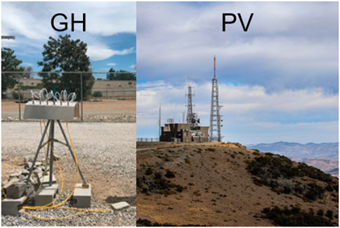
From 11/21/19 (month/day/year) to 11/24/20, two RMAS were deployed along with a Tekran 2537B to determine GOM, PBM, RM, and GEM at the University of Nevada, Reno Valley Road Greenhouse Complex [GH; 39.5375 N latitude, 119.8047 W longitude, elevation 1,368 m above sea level (masl)]. A fire event impacted Reno from 08/18/20 to 09/15/20 with two periods of heavy smoke. From 09/29/22 to 11/03/22, two RMAS were deployed simultaneously at the GH and on Peavine Peak (PV; 39.589389 N, 119.928797 W, 1940 masl).

A Tekran 2537B, used to measure GEM, was operated and maintained following protocols used by the National Atmospheric Deposition Program Atmospheric Mercury Network. The RMAS consists of a 25.4 mm-thick bent, anodized aluminum weather shield housing six dual- or triple-stage perfluoroalkoxy alkane (PFA) filter packs connected to vacuum pumps (KNF Neuberger Inc., 34 L per minute (Lpm) capacity; and Welch) stored inside or in a pump box. Ambient air flow was controlled by critical flow orifices (Teledyne API) at 1 Lpm, nominal. Flow rates through each filter pack were checked at the beginning and end of each deployment. All flow measurements were normalized to represent air flow at standard temperature and pressure conditions (0°C and 1 atm). For details, see Luippold et al. (2020b). Membranes used to collect GOM and PBM were cation exchange membranes (CEM; 0.8 μm pore size; Mustang-S, Pall Corporation^®) and polytetrafluoroethylene (PTFE) membranes (0.2 μm pore size, 47 mm diameter; Sartorius Stedium Biotech^®), respectively.

One RMAS was configured to measure RM concentrations and chemistry using triplicate two-in-line CEMs and triplicate two-in-line nylon membranes (0.2 µm pore size, Sartorius) in dual-stage filter packs, respectively. The second RMAS was identical to the first system, but used triple-stage filter packs that allowed for a PTFE membrane upstream of the two CEM or nylon membranes. The PTFE membrane was used to separate PBM (>0.2 μm) from GOM. Fourteen-day sampling periods were conducted from 12/17/19 through 07/15/20, and seven-day sampling periods occurred from 11/11/19 to 12/17/19 and 07/15/20 to 11/24/20. Deployment durations of 14 days during the winter were utilized due to low RM concentrations, and in the spring of 2020 were a result of institutional restrictions as a result of the COVID-19 pandemic.

Analyses

CEM, PTFE, and downstream nylon membranes were analyzed for total Hg following EPA Method 1631, Revision E (United States Environmental Protection Agency, 2002). Hg compounds were released by thermal desorption from upstream nylon membranes with subsequent thermal reduction through pyrolysis (388°C) to GEM and analyzed by cold vapor atomic fluorescence spectrometry using a Tekran 2537A (detection limit <0.1 ng·m^-3). For details about both methods, see the Supplementary Material. It is important to note that compounds desorbed are described as specific classes of compounds (i.e., –O, –N, –S, halogenated, and organic). Since HgBrNO₂ and HgBrOH are thought to be abundantly produced in GEM oxidation (Shah et al., 2021), it is uncertain whether these would be identified as a N, halogen, or O-based Hg^II compound. More sophisticated methods are under development (e.g., GC-MS) to more definitively identify these compounds; however, until those methods have been developed and vetted for accuracy, the thermal desorption system presented here provides a basis for understanding RM compounds.

HYSPLIT back trajectories

Back trajectory simulations were performed for each sampling period for this study using the NOAA Air Resources Laboratory GDAS1^o data archive and Hybrid Single-Particle Lagrangian Integrated Trajectory (HYSPLIT) model (http://ready.arl.noaa.gov/HYSPLIT.php, last access: 2023). Trajectories for the time of sampling were performed using a gridded frequency distribution method (Gustin et al., 2023). Trajectories were initiated every 4 h (00:00, 04:00, 08:00, 12:00, 16:00, 20:00 PST) from 9 points within a 0.5° × 0.5° horizontal grid centered on each site with four arrival heights (500, 1,000, 1,500, 2,000 magl), resulting in 216 trajectories per day. Generating a large number of trajectories provides for a reasonable representation of air mass transport (Stohl et al., 2002; Stohl et al., 2003; Weiss-Penzias et al., 2006).

Trajectory residence times were calculated for 6 source boxes (Eurasia, East Asia, north western and north eastern Pacific Ocean, Canada, and the United States; coordinate boundaries can be found in Supplementary Table S1). The boundary layer height was defined as 2,000 magl. Mixed layer depth was calculated in HYSPLIT. Two categories of trajectories were calculated for this study: 1) Twenty-four-h trajectories were generated to look at the path of regional air masses, and were calculated for the 24-hour period immediately before sample collection; and 2) trajectories were also calculated for the entire sampling duration (7 or 14 days) in order to determine the residence time of the sampled air that was above and below 2 km altitude and in the 6 source boxes. The 2 km boundary layer height was chosen because, due to high convective mixing, this is a typical boundary layer height for Reno.

Ancillary data

Criteria air pollutant and meteorological data were downloaded from local monitoring stations. For complete details, see the Supplementary Material. During the PV-GH comparison, ancillary data for the GH site were obtained from the same locations as for the year-long measurements.

Statistical analyses and modeling

Statistical analyses, including correlations, regressions, and t-tests, were performed in Microsoft Excel using the data analysis tool.

A generalized linear model (GLM) was applied to better understand factors impacting RM chemistry. Response variables (RM, GOM, PBM, and specific chemistry of compounds) were modeled separately as a function of predictor variables (Supplementary Table S2). Predictor variables were first removed to maintain pairwise correlations (Pearson’s ρ) ≤ 0.8 to reduce multicollinearity. For each response variable, a recursive feature elimination procedure was used (‘rfe’ function, with Random Forest method) and implemented in the ‘caret’ package (Kuhn, 2020) in R (R Core Team, 2020; version 4.0.2) to identify the set of predictor variables that optimized predictive performance under repeated cross-validation. Then, each response variable was modeled as a log-linear function of the top predictor variables identified above using a GLM with Gamma error distribution and an offset term (log of the number of sampling days) to account for differences in sampling effort. Finally, reverse stepwise selection was used to remove any non-influential regression terms using Akaike’s Information Criterion (Burnham and Anderson, 2002) as a model selection criterion. For each model, multiple goodness-of-fit tests were implemented in the ‘DHARMa’ package (Hartig, 2022) in R, including tests for uniformity of residuals, outliers, and overdispersion. The GLM was applied to similar data collected with RMAS at two additional field sites: 1) near Great Salt Lake at two locations, one adjacent to the lake at Antelope Island State Park marina (AISP; 41.060451 N, 112.238430 W, 1,283 masl) and another 11 km directly east of Antelope Island State Park location (41.084985, −112.111791, 1,288 masl); and 2) Georgia Tech campus in Atlanta, adjacent to a 14-lane highway (33.778463, −84.391425, 286 masl) (Gustin et al., 2023).

Results and discussion

General trends

In general, RM concentrations during this study were highest in the spring/summer (80–170 pg·m⁻³), and lower in the fall/winter (20–80 pg·m⁻³; Figures 1, 2). Comparing RMAS data from Gustin et al., 2023; October 2019 to January 2020), concentrations of up to 300 pg·m⁻³ were observed in October and declined to 25 pg·m⁻³ in January. Luippold et al. (2020a) and Luippold et al. (2020b) presented RMAS data from 2018 to 2019, with RM concentrations of 100–150 pg·m⁻³ from June to the end of October. Peterson et al. (2009) reported on Tekran Hg measurements made over 3 years (2005–2007) at Desert Research Institute (39.57 N, 119.80 W, 1,509 masl), 5 km north and 165 m above the GH site. Concentrations were highest in the summer, with the 3-year average for GOM being 26 ± 35 pg·m⁻³, and ranging between 0 and 401 pg·m⁻³. They also noted a diel pattern, with higher concentrations during the day, similar to ozone. Lyman and Gustin (2008) found, when comparing Tekran data collected at Desert Research Institute with that from a location 9 km east of Reno, that increased concentrations of GEM and PBM occurred when there was little atmospheric mixing, and suggested local sources were important for enhancing GEM and PBM concentrations in Reno. Concentrations of GOM and PBM measured with a Tekran system in Reno were on average 18 ± 22 and 7 ± 7 pg·m⁻³ (maximum of 177 pg·m⁻³), respectively, and were higher during periods with higher temperature and lower dew point. Lyman and Gustin (2008) suggested higher GOM concentrations at the DRI location support the hypothesis that subsiding dry air from the free troposphere was a source of GOM to the surface.

FIGURE 1

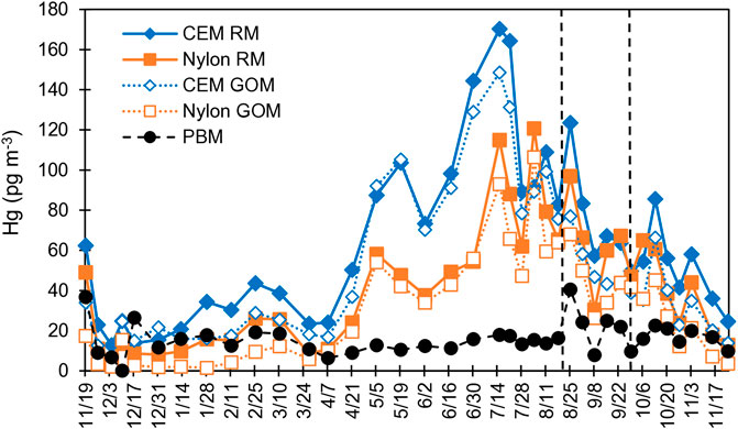
FIGURE 1. Time series of the CEM and nylon membrane-derived RM and GOM concentrations for the GH. PBM was derived from upstream PTFE membranes. Vertical lines delineate the start (left) and end (right) of the fire event. Dates indicate sample harvest dates.

FIGURE 2

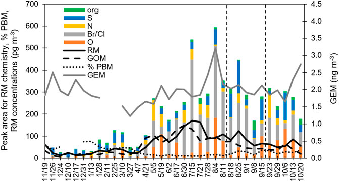
FIGURE 2. Time series of data developed at the GH: RM concentrations measured with the CEM; GEM measured by the Tekran 2537; %PBM, as determined using the Hg concentration on the PTFE membrane divided by the total Hg concentration for the PTFE membrane plus both CEM; and peak area for the different Hg^II compounds; and maximum mixing height (magl), calculated using HYSPLIT. Lines delineate the start (left) and end (right) of the fire event. Dates indicate sample harvest dates. Columns represent the RM chemistry based on peak area.

Spring and summer

From 05/05/2020 to 07/21/20, RM concentrations were typically >100 pg·m⁻³ (Figure 1). During this time, halogenated compounds were dominant, making up 45%–78% of the compounds measured (Figure 2; Supplementary Material). Other compounds present were O, N, and S, with percentages varying week-to-week. Oxide-Hg^II compounds were, in general, higher during this time (Supplementary Figure S1; Supplementary Table S3). Organic compounds were typically ∼5%.

High RM has been found to be associated with the tropopause (Lyman and Jaffe, 2012). NOAA operated their Tunable Optical Profiler for Aerosol and oZone lidar (TOPAZ) on June 17, 23, 24, and July 1, 2, 6, 8, 9, 10, and 16-17-2020. Elevated ozone layers consistent with stratospheric intrusions were observed on June 24 and July 8, but both remained above 7,000 masl and would not have impacted the surface anywhere near the sampling location (Andrew Langford, NOAA, personal communication). Thus, oxide compounds were not derived from the stratosphere.

During spring/summer, temperature and absolute humidity (or the mass of H₂O vapor per air volume) were higher, while RH (water vapor present relative to the amount of water needed for saturation) was lowest (Supplementary Figure S2) relative to the fall/winter. Wind speeds were also highest in the spring. Ozone concentrations were higher (50 ppbv) in the summer, compared to the fall/winter (30–40 ppbv; Figure 3). Fine et al. (2015) reported on sources of ozone to Nevada and found peak ozone concentrations in late spring to early summer across the state due to long-range transport.

FIGURE 3

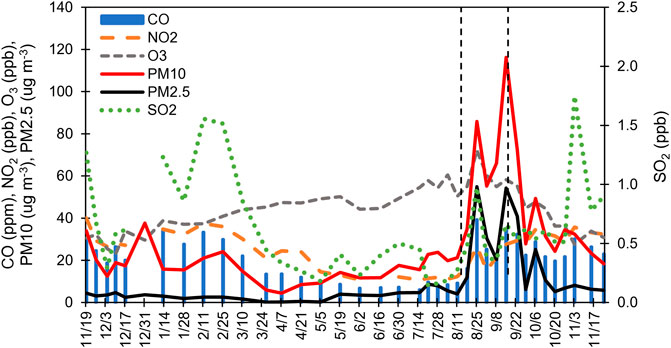
FIGURE 3. Criteria air pollutants measured by Washoe County and uploaded from EPA’s Air Quality System database for the duration of the sampling campaign. Lines delineate the start (left) and end (right) of the fire event. Dates indicate sample harvest dates.

Most of the trajectory analyses during the spring and summer were done over the 14 days of sampling, with the exception being 07/21/20 (7 days). Trajectories for the duration of sampling were primarily (>50%) situated over the Pacific Ocean, with few exceptions (Supplementary Table S4). Mixing heights were higher during this time than in fall/winter (Supplementary Figure S3), which would allow for capture of air masses entering the area from >2,000 magl. The dry air and higher temperatures promoted vertical mixing. Ozone concentrations were also higher, indicating inputs from the free troposphere (cf. Fine et al., 2015).

Twenty-four h trajectories showed that when air masses originated from generally unpolluted areas, S-Hg^II compounds were present, suggesting, in this case, these compounds are not regionally sourced and were associated with long-range transport. When air was primarily over the United States and the Pacific Ocean (e.g., July and August), S-Hg^II compounds were less abundant. This suggests that Eurasia/Asia was a likely source of these compounds. VanCuren and Gustin (2015), in a study investigating sources of ozone, using Interagency Monitoring of Protected Visual Environments network data, to Lassen and Great Basin National Parks, found that long-range transport contributed SO₄ aerosol that was associated with soil with reacted sea salt, mineral-bound SO₄, and mineral-bound NO₃. S-Hg^II compounds were primarily aerosol (Figure 4).

FIGURE 4

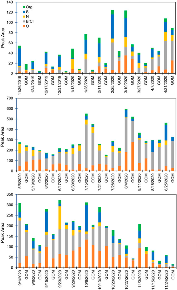
FIGURE 4. Peak areas of deconvoluted thermal desorption profiles for the specific compounds from nylon membranes at GH. Data associated with a date are RM measurements, with the corresponding GOM measurement to the right for the same sampling period. Dates indicate sample harvest dates.

Since during this time long-range transport was the dominant air movement, and high convective mixing occurred, this indicates that halogenated compounds were derived from the marine boundary layer, and oxide and sulfur compounds were derived from long-range transport.

Fall and winter

During the fall and winter, RM concentrations were lower (<80 pg·m⁻³) compared to spring/summer (Figure 1). CEM PBM was 40%–78% of RM, while from May to early September it was typically less than 20% (Figure 2). This indicates that during the fall/winter, local and regional pollution affected Reno air, while in the spring/summer, air from the free troposphere with little particulate matter was important. From mid-November through March, when sampling durations were predominantly 7 days, S-Hg^II compounds made up the highest percentage of RM compounds, ranging from 30% to 78% of total RM. In general, as PBM decreased so did S-Hg^II-based compounds, based on both peak area and proportion (Figure 2; Supplementary Material). S-Hg^II compounds also were highest for RM, indicating most of the S-based compounds were present as aerosol (Figure 4). It is important to note that when using the 7-day trajectories, we were not accounting for the air mass additions beyond the 7-day analyses, thus other areas could have contributed.

Oxide, N, halogenated, and organic-based Hg^II compounds were each typically 20% or less of the total RM, with a few time periods when values were higher. Oxide-based Hg^II compound concentrations were low in general, except for the fall 2020 when they were 25%–45% of the compounds present and long-range transport was important. For one sampling period, they were the dominant compound (5/19/20). O and halogenated compounds were often higher in concentration on the nylon membrane after the PTFE membrane, but not regularly, indicating the chemistries of PBM and GOM were different. This was not true for other compounds.

Local SO₂ concentrations were highest in the fall/winter, with concentrations up to 1.8 ppb, compared to spring/summer (<0.6 ppb; Figure 3). CO similarly had higher concentrations in the fall/winter (40 ppm) compared to the spring/summer (20 ppm). NO₂ concentrations were higher in the fall and winter (30 ppb), versus 10 ppb in spring/summer. During fall and winter, N-Hg^II compound peak areas were 10%–20%, higher than spring/summer when they were typically <10%.

During this time, maximum mixing heights were ∼1,500–2,000 magl, lower than the spring/summer (2,000–4,000 magl; Supplementary Figure S3). Many of the 24 h trajectories during this time were from urban areas, including San Francisco-Sacramento (Supplementary Table S3), suggesting regional transport of Hg^II compounds. Since air masses from these highly populated areas were directly impacting Reno, it is possible these areas contributed to the observed oxide, N, and S-Hg^II compounds. Because PBM was high, and local SO₂ and NO₂ concentrations were also high, it is possible that N and S-Hg^II compounds were produced locally. In the winter, Reno is prone to inversions, and smoke and exhaust from wood burning is captured in the stagnant air mass. This also fits in with the observation by Lyman and Gustin (2008) that Tekran-based PBM measurements increased when there was little mixing in the valley where Reno is situated.

Specific membrane details

Percent PBM collected on the PTFE membrane in front of the nylon membrane was typically higher than that on the PTFE in front of the CEM (Supplementary Figure S4; Nylon PBM = 0.8 * CEM PBM, r² = 0.79, p < 0.001), due to the fact that the nylon membrane does not capture all compounds with equal efficiency, and typically exhibits lower concentrations than the CEM (Figure 1).

Nylon and CEM with and without upstream PTFE membranes demonstrated similar trends in concentrations (Figure 1). CEM and CEM + PTFE were correlated (CEM + PTFE = 1.0 * CEM, r² = 0.96 p < 0.001), as were nylon and nylon + PTFE (nylon + PTFE = 1.1 * nylon, r² = 0.95, p < 0.001). On average, nylon membranes were less efficient at capturing Hg^II than the CEM by 34%, as previously noted for this location (Gustin et al., 2023; Dunham-Cheatham et al., 2023). During the winter, the disparity between the concentrations measured on the CEM and nylon membranes was ∼20 pg·m⁻³, while in the spring this increased to 40 pg·m⁻³ (Figure 1), indicating that during spring there were compounds present the nylon membrane was not efficiently capturing. Breakthrough was consistent for both membrane types across the sampling period (for details see the Supplementary Material), indicating that the forms not being captured were likely reduced on the nylon membrane.

Specific case studies

Percent PBM for the PTFE membranes in front of the nylon and CEMs were most similar during the fire event (08/18/20 to 09/15/20; Supplementary Figure S4). PM_2.5 during the study was typically 5–10 and PM₁₀ was 20–40 μg·m⁻³, while concentrations during the fire were 30–55 and 120–160 μg·m⁻³, respectively. Percent PBM increased to 30% during time periods when Reno was heavily impacted by wildfire smoke (Figures 1, 2). During this fire event, PM_2.5 and PM₁₀ exceeded U. S. Environmental Protection Agency Air Quality Standard for PM_2.5 of 15 μg·m⁻³ during distinct time periods (August 16, 19–23, 25, 27–30, September 3, 7, 11–17, 2020; Washoe County, 2021). S-based Hg^II compounds increased during the fire event, corresponding with increases in GEM and PBM, indicating the potential for generation of these compounds associated with fire events (Figures 2; Supplementary Material). NO₂, CO, and SO₂ concentrations also increased during the fire event (Figure 3). RM and GOM concentrations did not increase. When sampling in fire plumes, elevated GOM concentrations have not been measured (cf. Friedli et al., 2003). Observations indicated that RM chemistry could reflect inputs due to fire events, likely due to production of aerosol-based S-Hg^II compounds.

On 1/13/20, the 24 h trajectory showed air moving over the Pacific and Sacramento (Supplementary Figure S5). Halogenated, S, O, N, and organic-Hg^II compounds were 1, 3, 18, 40, and 38%, respectively, of the total RM chemistry (Supplementary Table S3), and PBM was 77% of the total RM concentrations. Trajectories showed air at < 2 km traveled over the Pacific Ocean and United States. During this time, the 14-day trajectories were fast-moving, starting north of Reno and traveling around the Northern Hemisphere over Eurasia. The high % PBM and lack of halogenated compounds suggests that S, O, N and organic-Hg^II compounds were derived regionally.

On 2/11/20, halogenated compounds were 11% of the RM compounds (Supplementary Table S3), while S-Hg^II compounds were high (40% of RM), and PBM was 41%. Twenty-four h trajectories showed that air was transported into the sampling location from rural areas in central Oregon and Washington (Supplementary Figure S5). Trajectories indicated that air <2 km was primarily over the United States and >2 km originated in Eurasia, then traveled over the Pacific Ocean into the United States. This suggests long-range transport as the origin of the S-based RM compounds.

On 5/19/20, O compounds were the dominant RM compound (48%), and Br/Cl (12%), N (25%), and S (10%) compounds were present at lower concentrations. PBM during this sampling period was low (10%). Twenty-four h trajectories indicated air moved in from the Central California Coast, over the Sierra Nevada Mountains, and into Reno (Supplementary Figure S5). Trajectories indicated that air at < 2 km passed primarily over the Pacific Ocean with some interaction with Asia/Eurasia at both below and above 2 km. Oxide and halogenated compounds were likely derived from the free troposphere and marine boundary layer, respectively, with N and S compounds coming from regional sources. S compounds could also be sourced from the marine boundary layer.

Lastly, for the week ending 10/6/20, O and S compounds were dominant, while N, halogenated, and organic compounds were <10%. The 24-h trajectory showed air moving in from San Francisco and Sacramento, while trajectories originated over the United States for <2 km (40% of the trajectory points) and predominately over the US for the >2 km (38%) with less time over the Eastern Pacific Ocean (Supplementary Figure S5). This suggests a local/regional source for these compounds.

Peavine-greenhouse comparison

In the 2022 PV-GH comparisons, samples were collected weekly and on the same day at both locations. RM concentrations at PV and GH ranged from 33 to 182 and 32–80 pg·m⁻³, respectively (Supplementary Figure S6 top panel). Concentrations decreased as temperatures cooled and a storm front moved in. RM concentrations at PV were always higher than at GH, except for the last sampling period due to the fast-moving storm that came in during the previous sampling period with average wind speeds of 2.3 m·s⁻¹ that was followed by 0.2 mm of precipitation; concentrations at the GH and PV were the same during this time due to turbulent mixing, and RM concentrations decreased due to removal by precipitation.

PBM concentrations were always higher at the GH (9–45 pg·m⁻³) than at PV (4–6 pg·m⁻³), with the exception being the time period impacted by the storm event when it was 6 and 5 pg·m⁻³, respectively. The higher concentrations at the greenhouse were due to local aerosol production.

Comparing the chemistry for the two locations demonstrated that O-Hg^II compounds were dominant during the sampling campaign, with Br/Cl, N, S, and organic compounds being of lesser amounts (Supplementary Figure S7). High O compounds were likely due to long-range transport that occurred during this time. Concentrations of O-Hg^II compounds were greater at PV than at GH, as were Br/Cl compounds at times, while N, S, and organic compounds were similar in concentration between the two locations (Supplementary Figure S7). For the last sampling event, chemistry and total peak area for both locations were the same due to mixing with the storm event. Since O compounds were typically highest for PV relative to the GH, it is thought that this was derived from outside of the basin. Br/Cl, N, S, and organic compounds were comparable in concentration or at times higher at the GH relative to PV. These compounds could have been derived from the valley and transported to PV by upslope winds. This is supported by maximum mixing heights of 2,000–3,000 m that were well above the top of Peavine Peak that is 570 m above Reno (Supplementary Figure S3).

GLM model results

The model was developed using the 2019–2020 GH dataset presented here. A goal was to see if a model developed from one location could be applied to accurately predict observations at other locations. The model was applied to two datasets, one developed at Guadalupe Mountains National Park and one for a site adjacent to a highway in Atlanta, Georgia (Gustin et al., 2023).

Response variables included RM, GOM, PBM, and the chemistry of the compounds. These were compared with meteorology, percent of trajectory points in source boxes, and criteria pollutants (Supplementary Table S2). The major influencing factor that was correlated with most variables was temperature, and was removed from model consideration. Another strongly correlated variable was NO₂, so the model was performed with and without this variable. Supplementary Table S7 provides details of the analyses, along with the webpage where the model is available.

RM and GOM concentrations were positively correlated with absolute humidity and ozone, all of which increase in the summer, and negatively correlated with CO that decreases in the summer. RM and GOM were also negatively correlated with NO₂ concentrations, that was a major driver of the model and decreased in the summer.

In terms of chemistry, O and N-Hg^II compounds were correlated with ozone. Br/Cl compounds were correlated with ozone and absolute humidity, due to the Br/Cl compounds dominating in the summer when ozone was higher and RH lower. S and organic-Hg^II compounds were positively correlated with PM_2.5, and S compounds were linked with transport from Eurasia. Besides these correlations, the GLM did not result in any conclusions that would help predict concentrations nor sources of RM based on ancillary data measurements and HYSPLIT trajectories. Lastly, the GH GLM did not accurately predict observations at the other locations, indicating that a singular simplistic GLM approach cannot be developed from a dataset from one location and applied universally.

Conclusion

There are several caveats to consider regarding use of data collected using the RMAS system. Since we are not certain regarding the exact chemistry of the RM compounds and the membrane measurements have not been calibrated, the interpretation of the chemistry observed with the RMAS system must be used with caution. In addition, RM concentrations collected with the CEM are underestimated based on the intercomparison conducted with a calibrated DCS (Dunham-Cheatham et al., 2023). The nylon membrane does not collect all compounds with equal efficiency. It is also possible that GOM could be captured on particulates collected on the PTFE membrane.

Based on data analysis, N compounds were locally/regionally sourced, while S compounds were derived from long-range transport, fires, regional production, local production, and possibly from the marine boundary layer. This suggests that chemistry associated with highway smog production could lead to formation of RM compounds. O compounds were derived from long-range transport, and halogenated compounds were from the marine boundary layer. This work showed that RM may also be derived and/or produced from both local and regional air masses. This is an important point that modelers should consider. This lack of prediction of RM concentrations and chemistry by the GEOS-Chem model is demonstrated in a forthcoming paper (Gustin et al., 2023).

Most of the mechanisms and products for production of RM are uncertain. Theoretical calculations suggest that in the atmosphere, GEM can be converted to Hg^II compounds by a mechanism that requires multiple oxidation steps involving Br and OH^* (Shah et al., 2021). Recently, Castro et al. (2022) suggested that OH^. and ozone together account for significant conversion of Hg(0) to Hg^II. The compounds defined in this work are not explained in theoretical calculations. Thus, being able to definitively identify the compounds would greatly improve our understanding of RM and GOM chemistry.

The GLM modeling exercise showed that each site requires its own data collection in order to create a model, thus more monitoring sites with the RMAS could help fill data gaps as new methods are developed that can better measure RM concentrations and chemistry. Lastly, despite the limitations of the RMAS data, it is a useful step in the path to more accurate and comprehensive measurements of Hg^II chemistry and concentrations.

Data availability statement

The original contributions presented in the study are included in the article/Supplementary Material. Further inquiries can be directed to the corresponding author.

Author contributions

MG compiled data for the paper and wrote the paper. SD-C collected the field data, analyzed the samples, and compiled data into spreadsheets and edited the paper. NC compiled all the HYSPLIT analyses and contributed to the paper. KS prepared the GLM model and ran the model. KS wrote modeling sections of the paper. NA did the Peavine-Greenhouse comparison and contributed to the paper. All authors contributed to the article and approved the submitted version.

Funding

Funding for this work was provided by the National Science Foundation, Grant Nos. 1700711 and 1700722.

Acknowledgments

The authors would like to thank Ben Ingle for his assistance with taking measurements and collecting samples throughout the sampling campaign; Lei Zhang and Weikang Zhang for their help validating the updated peak deconvolution method; and Andrew Langford of NOAA for investigating whether stratospheric intrusions were influencing observations. The authors thank the three reviewers for their constructive comments.

Conflict of interest

The authors declare that the research was conducted in the absence of any commercial or financial relationships that could be construed as a potential conflict of interest.

Publisher’s note

All claims expressed in this article are solely those of the authors and do not necessarily represent those of their affiliated organizations, or those of the publisher, the editors and the reviewers. Any product that may be evaluated in this article, or claim that may be made by its manufacturer, is not guaranteed or endorsed by the publisher.

Supplementary material

The Supplementary Material for this article can be found online at: https://www.frontiersin.org/articles/10.3389/fenvc.2023.1202957/full#supplementary-material

References

Ambrose, J. L., Lyman, S. N., Huang, J., Gustin, M. S., and Jaffe, D. A. (2013). Fast time resolution oxidized mercury measurements during the Reno atmospheric mercury intercomparison experiment (RAMIX). Environ. Sci. Technol. 47, 7285–7294. doi:10.1021/es303916v

PubMed Abstract | CrossRef Full Text | Google Scholar

Burnham, K. P., and Anderson, D. R. (2002). Model selection and inference: A practical information-theoretic approach. New York: Springer-Verlag.

Google Scholar

Castro, P. J., Kello, V., Cernusak, I., and Dibble, T. S. (2022). Together, not separately, OH and O₃ oxidize Hg⁽⁰⁾ to Hg^(II) in the atmosphere. J. Phys. Chem. A 126, 8266–8279. doi:10.1021/acs.jpca.2c04364

PubMed Abstract | CrossRef Full Text | Google Scholar

County (2021). 2011-20 Washoe county, Nevada air quality trends report. Available at: https://www.washoecounty.gov/health/programs-and-services/air-quality/air-quality-reports-and-data.php.

Google Scholar

Dunham-Cheatham, S. M., Lyman, S., and Gustin, M. S. (2023). Comparison and calibration of methods for ambient reactive mercury quantification. Sci. Total Environ. 856, 159219. doi:10.1016/j.scitotenv.2022.159219

PubMed Abstract | CrossRef Full Text | Google Scholar

Dunham-Cheatham, S. M., Lyman, S., and Gustin, M. S. (2020). Evaluation of sorption surface materials for reactive mercury compounds Atmospheric Environment. Atmos. Environ. 241, 117836. doi:10.1016/j.atmosenv.2020.117836

CrossRef Full Text | Google Scholar

Fine, R., Miller, M. B., Burley, J., Jaffe, D. A., Pierce, R. B., Lin, M. Y., et al. (2015). Variability and sources of surface ozone at rural sites in Nevada, USA: Results from two years of the Nevada rural ozone initiative. Sci. Total Environ. 530, 471–482. doi:10.1016/j.scitotenv.2014.12.027

PubMed Abstract | CrossRef Full Text | Google Scholar

Friedli, H. R., Radke, L. F., Lu, J. Y., Banic, C. M., Leaitch, W. R., and MacPherson, J. I. (2003). Mercury emissions from burning of biomass from temperate north American forests: Laboratory and airborne measurements. Atmos. Environ. 37, 253–267. doi:10.1016/s1352-2310(02)00819-1

CrossRef Full Text | Google Scholar

Gustin, M. S., Allen, N., Dunham Cheatham, S. M., Choma, N., Lyman, S. N., Johnson, W., et al. (2023). Observations of the chemistry and concentrations of reactive Hg at locations with different ambient air chemistry. submitted to STOTEN.

Google Scholar

Gustin, M. S., Dunham-Cheatham, S. M., and Zhang, L. (2019). Comparison of 4 methods for measurement of reactive, gaseous oxidized, and particulate bound mercury. Environ. Sci. Technol. 53, 14489–14495. doi:10.1021/acs.est.9b04648

PubMed Abstract | CrossRef Full Text | Google Scholar

Gustin, M. S., Dunham-Cheatham, S. M., Zhang, L., Lyman, S., Choma, N., and Castro, M. (2020). Use of membranes and detailed HYSPLIT analyses to understand atmospheric particulate, gaseous oxidized, and reactive mercury chemistry. Environ. Sci. Technol. 55, 893–901. doi:10.1021/acs.est.0c07876

CrossRef Full Text | Google Scholar

Gustin, M. S., Huang, J., Miller, M. B., Peterson, C., Jaffe, D. A., Ambrose, J., et al. (2013). Do we understand what the mercury speciation instruments are actually measuring? Results of RAMIX. Environ. Sci. Technol. 47, 7295–7306. doi:10.1021/es3039104

PubMed Abstract | CrossRef Full Text | Google Scholar

Gustin, M. S., Amos, H. M., Huang, J., Miller, M. B., and Heidecorn, K. (2015). Measuring and modeling mercury in the atmosphere: a critical review. Atmos. Phys. Chem. 15, 5697–5713. doi:10.5194/acp-15-5697-2015

CrossRef Full Text | Google Scholar

Hartig, F. (2022). DHARMa: Residual diagnostics for hierarchical (Multi-Level/mixed) regression models. Available at: https://CRAN.R-project.org/package=DHARMa.

Google Scholar

Huang, J., Miller, M. B., Weiss-Penzias, P., and Gustin, M. S. (2013). Comparison of gaseous oxidized Hg measured by KCl-coated denuders, and nylon and cation exchange membranes. Environ. Sci. Technol. 47, 7307–7316. doi:10.1021/es4012349

PubMed Abstract | CrossRef Full Text | Google Scholar

Jones, C. P., Lyman, S. N., Jaffe, D. A., Allen, T., and O'Neil, T. L. (2016). Detection and quantification of gas-phase oxidized mercury compounds by GC/MS. Atmos. Meas. Tech. 9–2205. doi:10.5194/amt-9-2195-2016

CrossRef Full Text | Google Scholar

Kuhn, M. (2020). caret: Classification and regression training. Available at: https://CRAN.R-project.org/package=caret.

Google Scholar

Luippold, A., Gustin, M. S., Dunham-Cheatham, S. M., Castro, M., Luke, W., Lyman, S., et al. (2020a). Use of multiple lines of evidence to understand reactive mercury concentrations and chemistry in Hawai’I, Nevada, Maryland, and Utah, USA. Environ. Sci. Technol. 54, 7922–7931. doi:10.1021/acs.est.0c02283

PubMed Abstract | CrossRef Full Text | Google Scholar

Luippold, A., Gustin, M. S., Dunham-Cheatham, S. M., and Zhang, L. (2020b). Improvement of quantification and identification of atmospheric reactive mercury. Atmos. Environ. 224, 117307. doi:10.1016/j.atmosenv.2020.117307

CrossRef Full Text | Google Scholar

Lyman, S. N., Elgiar, T., Gustin, M. S., Dunham-Cheatham, S. M., David, L. M., and Zhang, L. (2022). Evidence against rapid mercury oxidation in photochemical smog. Environ. Sci. Technol. 56, 11225–11235. doi:10.1021/acs.est.2c02224

PubMed Abstract | CrossRef Full Text | Google Scholar

Lyman, S. N., Gratz, L., Dunham-Cheatham, S. M., Gustin, M. S., and Luippold, A. (2020). Improvements to the accuracy of atmospheric oxidized mercury measurements. Environ. Sci. Technol. 54, 13379–13388. doi:10.1021/acs.est.0c02747

PubMed Abstract | CrossRef Full Text | Google Scholar

Lyman, S. N., and Gustin, M. S. (2008). Speciation of atmospheric mercury at two sites in northern Nevada, USA. Atmos. Environ. 42, 927–939. doi:10.1016/j.atmosenv.2007.10.012

CrossRef Full Text | Google Scholar

Lyman, S. N., and Jaffe, D. A. (2012). Formation and fate of oxidized mercury in the upper troposphere and lower stratosphere. Nat. Geosci. 5, 114–117. doi:10.1038/ngeo1353

CrossRef Full Text | Google Scholar

Mao, N., and Khalizov, A. (2021). Exchange reactions alter molecular speciation of gaseous oxidized mercury. ACS Earth Sp. Chem. 5, 1842–1853. doi:10.1021/acsearthspacechem.1c00178

CrossRef Full Text | Google Scholar

Osterwalder, S., Dunham-Cheatham, S. M., Araujo, B. F., Magand, O., Thomas, J. L., Baladima, F., et al. (2021). Fate of springtime atmospheric reactive mercury: Concentrations and deposition at zeppelin, svalbard. ACS Earth Space Chem 5, 3234–3246. doi:10.1021/acsearthspacechem.1c00299

CrossRef Full Text | Google Scholar

Peterson, C., Gustin, M. S., and Lyman, S. (2009). Atmospheric mercury concentrations and speciation measured from 2004 to 2007 in Reno, Nevada, USA. Atmos. Environ. 43, 4646–4654. doi:10.1016/j.atmosenv.2009.04.053

PubMed Abstract | CrossRef Full Text | Google Scholar

Rumayor, M., Diaz-Somoano, M., Lopez-Anton, M. A., and Martinez-Tarazona, M. R. (2015). Application of thermal desorption for the identification of mercury species in solids derived from coal utilization. Chemosphere 119, 459–465. doi:10.1016/j.chemosphere.2014.07.010

PubMed Abstract | CrossRef Full Text | Google Scholar

Rumayor, M., Diaz-Somoano, M., Lopez-Anton, M. A., and Martinez-Tarazona, M. R. (2013). Mercury compounds characterization by thermal desorption. Talanta 114, 318–322. doi:10.1016/j.talanta.2013.05.059

PubMed Abstract | CrossRef Full Text | Google Scholar

Shah, V., Jacob, D. J., Thackray, C. P., Wang, X., Sunderland, E. M., Dibble, T. S., et al. (2021). Improved mechanistic model of the atmospheric redox chemistry of mercury. Environ. Sci. Technol. 55, 14445–14456. doi:10.1021/acs.est.1c03160

PubMed Abstract | CrossRef Full Text | Google Scholar

Stohl, A., Eckhardt, S., Forster, C., James, P., Spichtinger, N., and Seibert, P. (2002). A replacement for simple back trajectory calculations in the interpretation of atmospheric trace substance measurements. Atmos. Environ. 36, 4635–4648. doi:10.1016/s1352-2310(02)00416-8

CrossRef Full Text | Google Scholar

Stohl, A., Forster, C., Eckhardt, S., Spichtinger, N., Huntrieser, H., Heland, J., et al. (2003). A backward modeling study of intercontinental pollution transport using aircraft measurements. J. Geophys. Res. 108, 4370. doi:10.1029/2002jd002862

CrossRef Full Text | Google Scholar

United States Environmental Protection Agency (Epa), (2002). EPA method 1631, revision E: Mercury in water by oxidation, purge and trap, and cold vapor atomic fluorescence spectrometry.

Google Scholar

VanCuren, R., and Gustin, M. S. (2015). Identification of sources contributing to PM2.5 and ozone at elevated sites in the Western US by receptor analysis: Lassen volcanic national Park, California, and Great Basin National Park, Nevada. Sci. Total Environ. 530, 505–518. doi:10.1016/j.scitotenv.2015.03.091

PubMed Abstract | CrossRef Full Text | Google Scholar

Weiss-Penzias, P., Jaffe, D. A., Swartzendruber, P., Dennison, J. B., Chand, D., Hafner, W., et al. (2006). Observations of Asian air pollution in the free troposphere at Mount Bachelor Observatory during the spring of 2004. J. Geophys. Res. 111, D10304. doi:10.1029/2005jd006522

CrossRef Full Text | Google Scholar