Generation of typical scenarios for distribution networks in planning stage considering photovoltaic and load growth characteristics

With the increasing integration of distributed rooftop photovoltaic (PV) systems into distribution networks, traditional scenario generation methods based solely on historical PV data have become inadequate. This paper proposes a planning-stage PV scenario generation method to address the challenges of high-penetration rooftop PV integration. The method combines Conditional Generative Adversarial Networks (CGAN) with an improved Bass model to estimate new PV capacity. Load scenarios are constructed by analyzing regional load growth patterns. Typical weather days are classified using Spearman’s rank correlation coefficient to form joint PV-load scenarios, which are then reduced using k-means clustering. The study compares multi-scenario energy storage configuration schemes considering planning-stage scenarios with those based only on historical data predictions. Results demonstrate that the generated planning-stage scenarios align well with future actual operating scenarios. Furthermore, the energy storage configuration scheme considering planning-stage scenarios outperforms the scheme based solely on historical data predictions, indicating the proposed method’s effectiveness in addressing high-penetration PV integration challenges in distribution network planning.

1 Introduction

In the context of widespread photovoltaic (PV) application, an increasing number of rooftop distributed PV systems are being continuously integrated into distribution net-works (Uddin et al., 2023). The power output of distributed PV systems exhibits significant randomness and strong correlation with meteorological conditions (Wang et al., 2023). Generating reasonable planning-stage PV and load scenarios for distribution networks with rooftop PV systems has become a challenging issue in terms of enhancing local PV consumption and ensuring secure and reliable system operation.

For planning distribution networks with PV integration, the typical scenario generation method is commonly used (Ehsanbakhsh and Sepasian, 2023; Lefeng et al., 2022). This method extracts representative characteristics of PV and load data while reducing the original large-scale PV and load scenarios, thereby obtaining a small number of representative typical scenarios. This approach achieves the transformation from numerous uncertain PV output scenarios to a few deterministic scenarios.

Currently, typical scenario generation methods can be classified into two main categories (Zhang et al., 2018). The first category employs traditional clustering algorithms, including K-means clustering based on Euclidean distance, spectral clustering based on graphs, and fuzzy clustering algorithms (Gao et al., 2017). Reference (Hu and Li, 2022) proposes an improved k-means clustering algorithm based on multi-feature indicators, extracting features from historical information of island power supply systems to generate PV scenarios. Reference (Yang et al., 2022) uses a clustering algorithm based on local density centers to analyze historical PV output data, taking cluster centers as typical output scenarios, and then utilizes Copula functions to establish formulas de-scribing correlations between typical scenarios.

The second category primarily involves artificial intelligence learning methods (Ali E and Qiang, 2019). These methods use neural networks with learning and fitting capabilities to learn the distribution characteristics of historical data, enabling the network to generate desired data sequences. Reference (He et al., 2022) proposes an improved generative adversarial network for PV scenario generation. Its designed loss function incorporates Lipschitz continuity constraints, enhancing the convergence speed of the scenario generation model and the quality of generated scenarios, capturing nonlinear characteristics of PV output. Reference (Niu et al., 2021) presents a random scenario generation method for renewable energy based on pixel convolutional generative networks. This method generates PV and wind power curves point by point through a chain method, verifying that the constructed output curves can effectively simulate the volatility and spatiotemporal correlation characteristics of actual wind and PV power.

Although these methods have shown good results in generating renewable energy scenarios, they mostly rely on historical scenarios as references. For distribution networks experiencing rapid integration of rooftop distributed PV, they fail to fully consider the growth characteristics of renewable energy output and load, and cannot establish operational scenarios oriented towards the planning stage. To address this issue, a common approach is to forecast renewable energy output and load. Reference (Chen et al., 2021) proposes a stochastic power multi-scenario prediction model based on Markov chains. It models and analyzes the stochastic characteristics of renewable energy and load, as well as seasonal fluctuations, and finally completes the prediction of renewable energy output and load levels based on a multi-scenario prediction model using scenario trees. Reference (Hu et al., 2022) first uses the BIRCH unsupervised clustering algorithm to divide historical data into datasets under three typical weather conditions, and then employs a dual-layer L-Transformer model to complete short-term PV power prediction. The model’s robustness and accuracy for different weather types are verified through measured data. Although predictions of PV and load can provide references for distribution network operation and planning, they still do not adequately address the issues brought by rapid integration of rooftop PV into distribution networks, nor can they form more specific planning-stage operational scenarios for distribution networks.

What’s more, current methods often treat PV generation and load growth as independent processes, neglecting their inherent correlations and the impact of external factors such as regional economic development and technological advancements. This limitation is particularly critical in the context of high-penetration PV integration, where the variability of PV output and the uncertainty of load growth can significantly affect the stability and reliability of distribution networks (Cheng et al., 2021; Colmenar-Santos et al., 2016).

To address these problems, this paper proposes a method for generating typical planning-stage scenarios considering PV-load growth characteristics (Cheng et al., 2024). For PV, it first uses a Conditional Generative Adversarial Network (CGAN) to fully learn the relationship be-tween PV capacity and output from historical PV data, and then employs an improved Bass model to estimate the relationship between future additional capacity and time, thereby completing the generation of PV output scenarios corresponding to specific PV capacities at future time cross-sections. For load, it first studies the load growth patterns of regional distribution networks to determine the growth situations of different load types (Zhu et al., 2024). Then, it combines historical load data to construct planning-stage load scenarios. Due to the strong correlation between PV, load, and meteorological factors, to achieve joint PV-load scenario generation, Spearman’s rank correlation coefficient is first used to analyze the correlations between meteorological factors and PV/load, completing the classification of typical weather days. Subsequently, the planning-stage PV and load scenario datasets are divided into different typical weather days. Finally, the k-means clustering algorithm is applied to different datasets to complete scenario reduction, obtaining joint typical PV-load scenarios for different weather days in the planning stage. By integrating these approaches, our method not only captures the dynamic growth characteristics of PV and load but also generates joint PV-load scenarios that reflect the correlations between meteorological conditions, PV output, and load demand. This represents a significant advancement over traditional methods, as it provides a more accurate and comprehensive framework for distribution network planning in the era of high-penetration renewable energy integration.

2 Materials and methods

2.1 Planning-stage PV scenario generation based on CGAN and bass model

For medium to long-term planning of distribution networks with rapidly increasing rooftop PV integration, it is crucial to generate PV output scenarios that align with future time cross-sections. Therefore, this paper proposes a planning-stage PV scenario generation method based on Conditional Generative Adversarial Networks (CGAN). First, historical PV operational data is used to train the CGAN network, enabling it to fully learn the relationship between PV output and capacity in the distribution network. Then, the Bass model is employed to estimate the installed capacity of rooftop PV in the distribution network area, fitting the relationship between additional PV capacity and time. Finally, the CGAN is equipped with the ability to generate planning-stage PV scenarios for future capacities (Cheng et al., 2020).

2.1.1 Conditional generative adversarial network

Generative Adversarial Networks (GAN) are unsupervised learning models, consisting of two structurally independent deep learning networks: a generator and a discriminator (Wenlong et al., 2022). Through adversarial learning between the generator and discriminator, the authenticity of samples generated by the generator is improved, enabling data-driven un-supervised learning.

The original GAN is an unsupervised model, generating uncontrollable data and exhibiting drawbacks in training stability and convergence, as well as being prone to local optima. Most importantly, GAN can only learn from provided historical training data, generating samples essentially consistent with the historical data, which is not well-suited for this paper’s goal of generating future scenario data driven by historical scenario data. CGAN, however, introduces a condition c, improving the network into a supervised model. During network training, each iteration of real data is input along with a condition c, allowing the generator to learn the correlation between the real data and condition c, in addition to learning the characteristics of the real data. This provides a de-gree of controllability for generating data under specific conditions (Yanping et al., 2023). The basic structure of the CGAN model is shown in Figure 1.

Figure 1

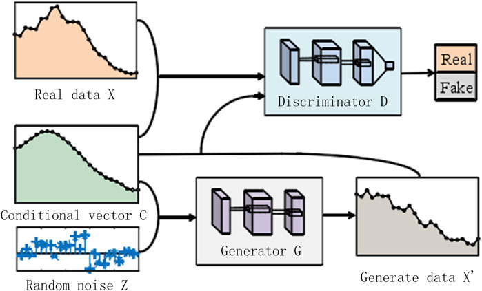
Figure 1. Basic structure of CGAN network.

The loss functions for the generator G and discriminator D are shown in Equations 1, 2, respectively.

${\mathrm{L}}_{\mathrm{G}}={-\mathrm{E}}_{z\sim p_z\left(z\right)}\left[\log \left(1-\mathrm{D}\left(\mathrm{G}\left(z\right)\right)\right)\right](1)$

${\mathrm{L}}_{\mathrm{D}}=-{\mathrm{E}}_{\mathrm{x}\sim {\mathrm{p}}_{\text{data}}\left(\mathrm{x}\right)}\left[\text{logD}\left(\mathrm{x}\right)\right]+{\mathrm{E}}_{\mathrm{z}\sim {\mathrm{p}}_{\mathrm{z}}\left(\mathrm{z}\right)}\left[\log \left(1-\mathrm{D}\left(\mathrm{G}\left(\mathrm{z}\right)\right)\right)\right](2)$

Where E represents the expectation of the distribution.

The objective function of CGAN is shown in Equation 3:

$\begin{array}{ll}\hfill \underset{\mathrm{G}}{\mathit{min}}\underset{\mathrm{D}}{\mathit{max}}\mathrm{V}\left(\mathrm{D},\mathrm{G}\right)& ={\mathrm{E}}_{\mathrm{x}\sim {\mathrm{p}}_{\text{data}}\left(\mathrm{x}\right)}\left[\log \mathrm{D}\left(\mathrm{x}\mid \mathrm{c}\right)\right]\hfill \\ \hfill & +{\mathrm{E}}_{z\sim p_z\left(z\right)}\left[\log \left(1-\mathrm{D}\left(\mathrm{G}\left(\mathrm{z}\mid \mathrm{c}\right)\mid \mathrm{c}\right)\right)\right]\hfill \end{array}(3)$

Where V(D,G) represents a binary cross-entropy function, aiming to minimize the Jensen-Shannon (JS) divergence between the probability distributions of generated samples and real samples (Jun et al., 2023).

The condition c not only provides direction for training data samples but can also serve as a classification label for training data. In this section, c is defined as the PV capacity value. Through the driving of historical PV output data under different capacities, the CGAN network is trained, enabling the generator to produce PV output data for specific capacities.

Since the randomness of PV output is mainly reflected in vertical similarity, i.e., PV output at a certain moment has a strong similarity with adjacent moments but little correlation with distant moments, convolutional neural networks are chosen to design the CGAN structure. This is because convolutional networks can adequately fit the correlation between a point and its nearby points without considering distant points.

2.1.2 Estimation of additional PV capacity in regional distribution networks based on bass model

This section studies the integration of rooftop PV in regional distribution networks, using the Bass model to fit the change of additional rooftop PV capacity over time. This determines the total installed capacity of rooftop PV at a future time cross-section, thereby constructing planning-stage PV output scenarios for the corresponding time.

2.1.2.1 Rooftop PV potential in regional distribution networks

For the same rooftop PV installation area, the capacity of different PV panels varies. As a device that converts solar energy into electrical energy, it is widely used in residential, commercial, and industrial sectors.

Since polycrystalline silicon PV panels are currently mainstream and their scale and advantages will not be easily surpassed by other types of PV panels for a long time in the future, this paper focuses on this type of PV panel. The maximum installed capacity (i.e., maximum PV potential) of PV panels is shown in Equation 4:

$E_p=S_r\times P_n\times H_A(4)$

Where $S_r$ is the total installable area of PV panels; $P_n$ is the rated power value of PV panels; $H_A$ is the solar radiation.

The total installable area of rooftop PV panels can be obtained from relevant departments of the power grid company, including rooftop information associated with each distribution area. Through the power grid’s supporting rooftop area identification technology, the total effective rooftop area available for PV installation can be obtained and converted into the total installable area of PV panels, ultimately completing the maximum installed capacity value associated with the distribution network’s rooftops.

Figure 2 shows the rooftops associated with a certain 10 kV feeder line in a region of Guangdong, with the red parts indicating the rooftop area available for PV panel installation. Table 1 shows the current transformer capacity and PV installed capacity for each node of this feeder line, while Table 2 shows the corresponding available rooftop area and potential installed capacity.

Figure 2

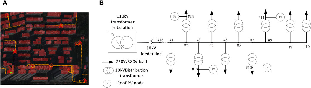
Figure 2. Identification of roof area associated with 10 kV feeder line: (A) The roof area associated with this feeder line; (B) 10 kV feeder topology diagram.

Table 1

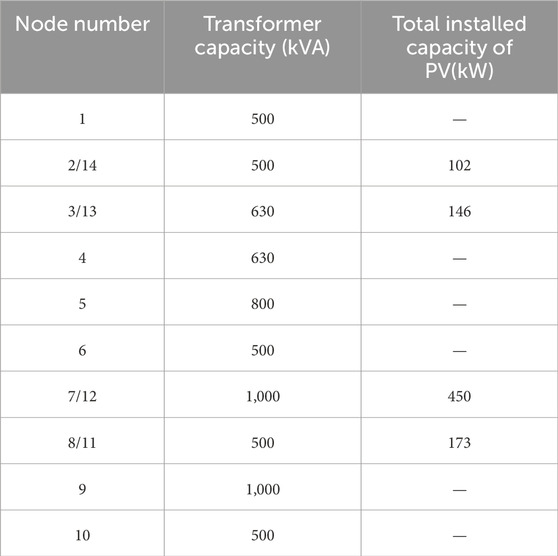
Table 1. Current transformer capacity and photovoltaic installed capacity of each node.

Table 2

Table 2. The available roof area and maximum installed capacity of this feeder line.

2.1.2.2 Estimation of additional capacity based on bass model

The main ideas of the Bass model based on the diffusion of innovative products are:

1. The diffusion process of innovative products is a process where potential groups gradually accept and use the product.

2. Potential groups are mainly divided into two categories: innovators and followers.

3. Innovators are easily influenced by external factors to adopt innovative products, while followers are easily influenced by internal factors to adopt innovative products (Zhangjin et al., 2021).

The logical relationship is shown in Figure 3:

Figure 3

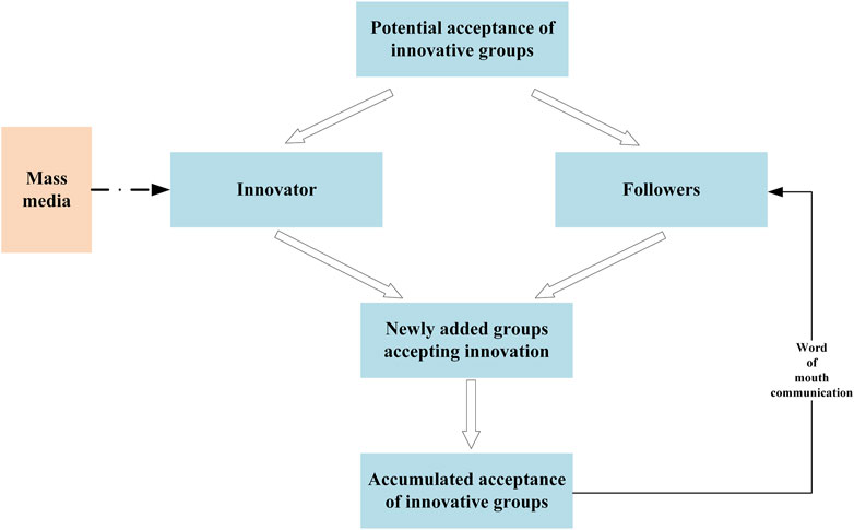
Figure 3. Schematic diagram of the logic flow of the Bass model.

In the field of rooftop PV diffusion, the Bass model can be improved by extracting its core ideas. Therefore, the three modeling elements of the improved Bass model can be analyzed as: $E_p$ is the installation potential of rooftop PV, innovation coefficient p, and imitation coefficient q. $E_p$ refers to the total capacity of rooftop PV ultimately installed; innovation coefficient p refers to the influence of the external environment on potential installation groups; imitation coefficient q refers to the influence of uninstalled groups imitating installed groups due to word-of-mouth and other spreading factors (Goodfellow I. et al., 2014).

Based on the modeling elements of the improved Bass model, the cumulative curve expression equation $N\left(t\right)$ and density curve expression equation $n\left(t\right)$ in the field of rooftop PV diffusion are shown in Equations 5, 6, respectively:

$N\left(t\right)=E_p\left[\frac{1-e^{-\left(q+p\right)t}}{1+\frac{q}{p}{e}^{-\left(q+p\right)t}}\right](5)$

$n\left(t\right)=E_p\left[\frac{p{\left(q+p\right)}^2{e}^{-\left(q+p\right)t}}{{\left[p+q{e}^{-\left(q+p\right)t}\right]}^2}\right](6)$

Where p is the innovation coefficient, q is the imitation coefficient, and $p,q\in \left[0,1\right]$.

Assuming that individual users will choose to install rooftop PV in time period t, based on the above Equation 5, the cumulative distribution function $F_T\left(t\right)$ related to t is shown in Equation 7:

$F_T\left(t\right)=\frac{1-e^{-\left(p+q\right)t}}{1+\frac{q}{p}{e}^{-\left(p+q\right)t}},t>0(7)$

In terms of rooftop PV diffusion, let g represent the user group connected to the same distribution network. The initial potential market $H_g$ represents the total number of users with sufficient roof resources and meeting the minimum economic conditions for rooftop PV installation, while the final potential market $F_g$ is the estimated number of users with economic potential and intention to install rooftop PV, i.e., the installation potential of the distribution network, which is a subset of $H_g$. Therefore, the calculation of $F_g$ can be done through Equation 8:

$F_g=M_g{H}_g(8)$

Where $M_g$ is the maximum market share of rooftop PV installation in group g. In other words, according to the analysis of PV technology diffusion in the study area and Equation 8, the number of customers in $F_g$ corresponds to the number of users in proportion $M_g$ in $H_g$.

The cumulative capacity $N_g\left(t\right)$ of rooftop PV can be obtained by Equation 9:

$N_g\left(t\right)=F_T\left(t\right)F_g(9)$

Where t represents a future time cross-section, and g is the user group connected to the same distribution network.

Through the above formula calculations, we obtain the estimated cumulative installed capacity of rooftop PV in the distribution network at a future time cross-section, addressing the lack of applicable planning-stage PV output scenario data for that time cross-section.

2.1.3 Planning-stage PV scenario generation for specific capacities

2.1.3.1 CGAN training steps

The PV output sampling interval in this study is 1 h. The training process of the CGAN planning-stage PV scenario generation model using historical PV operational data is as follows:

Step 1: Normalize historical PV output training sample data and historical PV capacity control conditions. Concatenate 1*24 dimensional noise following a standard normal distribution and 1*24 dimensional daily scenarios of real PV with historical PV capacity c. Process through convolutional kernels to output generated samples (Fake data) and real samples (Real data) containing condition c.

Step 2: Input Fake data and Real data into the discriminator network. The discriminator outputs discrimination results through the objective function and feeds back to the generator.

Step 3: Extract gradient penalty sampling points, calculate loss functions for G and D, and update their network weights.

Step 4: Determine if training is complete. If not, return to Step 1 and continue iteration.

Step 5: Training ends.

During training, the output of the discriminator in Figure 4 illustrates the evolution of the generated samples. Initially, generated samples (orange) and real samples (blue) are easily distinguishable by the discriminator. As the model progresses, they become increasingly difficult to differentiate. Figure 5 shows the distance between real and generated samples. When approaching zero, it indicates that the two distributions are close, suggesting that the distribution generated by the generator model is now close to the real PV output distribution, and training is complete.

Figure 4

Figure 4. Discriminator output change curve.

Figure 5

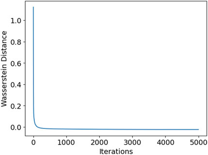
Figure 5. JS distance variation curve.

2.1.3.2 Planning-stage PV scenario generation

Obtain the cumulative installed PV capacity at a future time cross-section based on the Bass model. Extract the generator model trained with real historical data from Section 2.3.1. Use the cumulative installed PV capacity as the condition value c, input it along with high-dimensional noise following a normal distribution into the generator model. This ultimately yields rooftop PV output scenarios for each distribution area under that capacity, further obtaining planning-stage PV generation scenarios for each rooftop PV connection point in the distribution area.

The blue line in Figure 6 shows a historical daily PV operation scenario for a distribution area with a total rooftop PV capacity of 154 kW. When the total rooftop PV capacity of this area increases to 188kW, the corresponding planning-stage PV operation scenario for that day is shown by the red line. Similarly, in Figure 7, the old capacity is 170 kW and the new capacity is 195 kW.

Figure 6

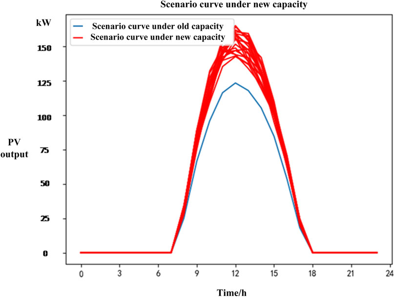
Figure 6. PV scenario for distribution area 1.

Figure 7

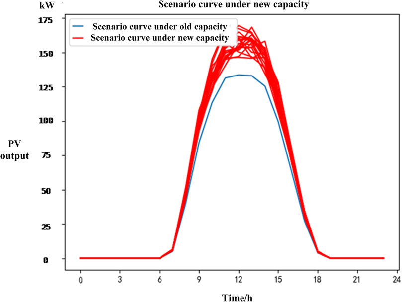
Figure 7. PV scenario for distribution area 2.

As shown in Figure 8, for node 7/12 of the feeder line in Figure 2, 365 daily PV operation scenarios are generated using the trained CGAN generator under a specific future PV capacity. The PV output has been normalized.

Figure 8

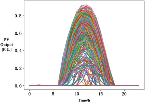
Figure 8. Generated planning-stage PV scenarios for a certain distribution area.

The proposed CGAN model, through its convolutional neural network architecture, captures the short-term variability of PV generation by learning the temporal correlations in historical PV output data. This allows the model to generate realistic hourly PV output scenarios that reflect the dynamic nature of solar power production. Additionally, the Bass model provides a framework for estimating future PV capacity growth, which, when combined with the CGAN-generated scenarios, accounts for long-term trends and seasonal variations in PV generation.

2.2 Construction of planning-stage load scenarios considering regional distribution network load growth characteristics

In this section, we focus on the construction of planning-stage load scenarios, taking into account the regional distribution network’s load growth characteristics. The approach involves categorizing loads into residential, commercial and industrial, agricultural, and office types, and estimating their growth rates based on historical data. This method inherently captures the diverse growth dynamics of each load type, which can exhibit non-linear trends due to varying socioeconomic factors.

By segregating loads into different categories, the model accounts for the unique growth patterns specific to each sector. For instance, residential load growth may be influenced by population dynamics and household electrification rates, while commercial and industrial loads might be affected by economic indicators such as GDP growth and industrial policy changes. This method thus allows for a nuanced understanding of load growth, reflecting the complex interplay of factors that drive demand in each sector.

Furthermore, the regional analysis in our model considers the specific characteristics of each sub-region, including local economic development and infrastructure expansion. This regional approach introduces variations in load growth patterns, acknowledging that different areas may experience distinct growth trajectories based on their economic and social contexts.

To construct planning-stage load scenarios, it is necessary to understand information such as load power and distribution at a future time cross-section. First, by studying the load growth patterns of specific regions and combining with existing loads, the load levels for a future period can be fitted, completing the construction of planning-stage load scenarios.

2.2.1 Load growth patterns

Load growth is an uncertain process, with different types of loads exhibiting distinct growth characteristics. However, loads in neighboring areas also have certain spatiotemporal correlations. Therefore, the key to constructing regional load growth patterns lies in distinguishing load types and determining the impact of load spatiotemporal characteristics on growth. This paper selects existing point load growth and large-capacity load application methods combined with spatiotemporal characteristics, using sequence operation theory to analyze and describe load growth (Goodfellow I. J. et al., 2014).

First, the loads in the studied area are categorized into four types: residential, commercial and industrial, agricultural, and office. The natural growth rates for each type are obtained through statistical analysis of historical load data from the distribution network data collection and monitoring system. Then, the natural growth rates are adjusted based on the development function positioning of the load area to determine the overall growth rate data for future loads, ultimately obtaining the total future load for each region and type.

To quantify the uncertainty of load growth and consider the differences in growth rates among different load types and regions, this paper establishes scenarios including high, low, and medium load growth. The studied area is divided into M sub-regions, with the load growth prediction value for sub-region k denoted as ${\mathrm{Q}}_{1\mathrm{k}}^{\mathrm{h}}、{\mathrm{Q}}_{1\mathrm{k}}^{\mathrm{m}}、{\mathrm{Q}}_{1\mathrm{k}}^1$ , and its corresponding probability as ${\mathrm{P}}_{1\mathrm{k}}^1,{\mathrm{P}}_{1\mathrm{k}}^{\mathrm{m}},{\mathrm{P}}_{1\mathrm{k}}^1\left(\mathrm{k}=1,2...,\mathrm{M}\right)$ . This is then discretized with a step size $\overline{Q}$, ultimately obtaining the probabilistic sequence formula $a_k\left(i\right),i=0,1,...,N_k$ for the sub-region as shown in Equations 10, 11:

$N_k=\left[Q_{lk}/\overline{Q}\right](10)$

$a_k\left(i\right)=\left\{\begin{array}{l}{P}_{lk}^{h}i=\left[Q_{lk}^h/\overline{Q}\right]\hfill \\ P_{lk}^{m}i=\left[Q_{lk}^m/\overline{Q}\right]\hfill \\ P_{lk}^{l}i=\left[Q_{lk}^l/\overline{Q}\right]\hfill \\ 0\text{else}\hfill \end{array}\right.(11)$

In Equation 10, $\left[x\right]$ represents the largest integer not exceeding x; $N_k$ is the number of discretized values for sub-region k. The superscripts h, m, and l represent high, medium, and low growth scenarios, respectively.

When considering the correlation between growth in different regions and load types, the total probability sequence $\mathrm{x}\left(\mathrm{i}\right)$ can be obtained according to the probability sequence derivation rule. By calculating the expected value of this sequence, we can obtain the expected value of total load growth as ${\mathrm{E}}_{\mathrm{Q}}$. Finally, the increased load is allocated according to the characteristics of load distribution, which can be expressed using Equations 12, 13:

$x\left(i\right)=a_1\left(i\right)\oplus a_2\left(i\right)\oplus ......\oplus a_m\left(i\right)(12)$

$E_Q=\overline{Q}{\displaystyle \sum _{i=0}^{N_0}}ix\left(i\right)(13)$

In Equations 12, 13, $N_0={\displaystyle {\sum }_{k=1}^M}{N}_k$; $\oplus$ represents the convolution sum operation.

For large user applications, the final total regional load growth prediction value is determined based on the installed load capacity $P_{cap}$ provided by the relevant power grid department, the load terminal utilization coefficient ${\alpha }_{pra}$, the stage coefficient $b_{sta}$, and considering the simultaneous rates of large user load ${\eta }_{ins}$ and regional load ${\eta }_{ng}$, determine the final total regional load growth forecast value $P_{Forecast}$, as shown in Formulas 14, 15:

$P_{install}=P_{cap}\times {\alpha }_{pra}\times b_{sta}(14)$

$P_{Forecast}={\eta }_{ng}\times \left(P_{Naturalgrowth}\left(E_Q\right)+{\eta }_{ins}\times P_{install}\right)(15)$

Through modeling and analysis of historical load data, as well as research on the distribution network load growth rate calculation model constructed based on regional characteristics, a series of load growth characteristics for a future time cross-section based on the actual situation of the regional distribution network are obtained.

2.2.2 Construction of planning-stage load scenarios

This section needs to integrate historical load scenarios and load growth characteristics, reasonably superimposing the load growth characteristics of the regional distribution network onto historical load scenarios. This updates a large number of historical load scenarios into planning-stage load scenarios that conform to a future time cross-section, laying the data foundation for forming typical planning-stage load scenarios.

Based on the above analysis, a load scenario prediction model oriented towards medium and long-term planning stages is established, as shown in Equation 16:

$M_t=M_{t_0}\times \left(1+\frac{P_{Forecast}-P_0}{P_0}\right)(16)$

Where $M_t$ represents the planning-stage daily load operation scenario for a future time cross-section; $M_{t_0}$ represents the historical daily load operation scenario; $P_{Forecast}$ is the load prediction value from Equation 15; $P_0$ represents the total regional load at the most recent time in the historical load data.

The blue lines in Figures 9, 10 show the daily load operation scenario for a distribution area with a transformer capacity of 1000kVA. Through the study of the load growth pattern in this distribution network area, the red line in Figure 9 shows the operation scenario for this distribution area’s load after 1 year, and the red line in Figure 10 shows the scenario after 2 years.

Figure 9

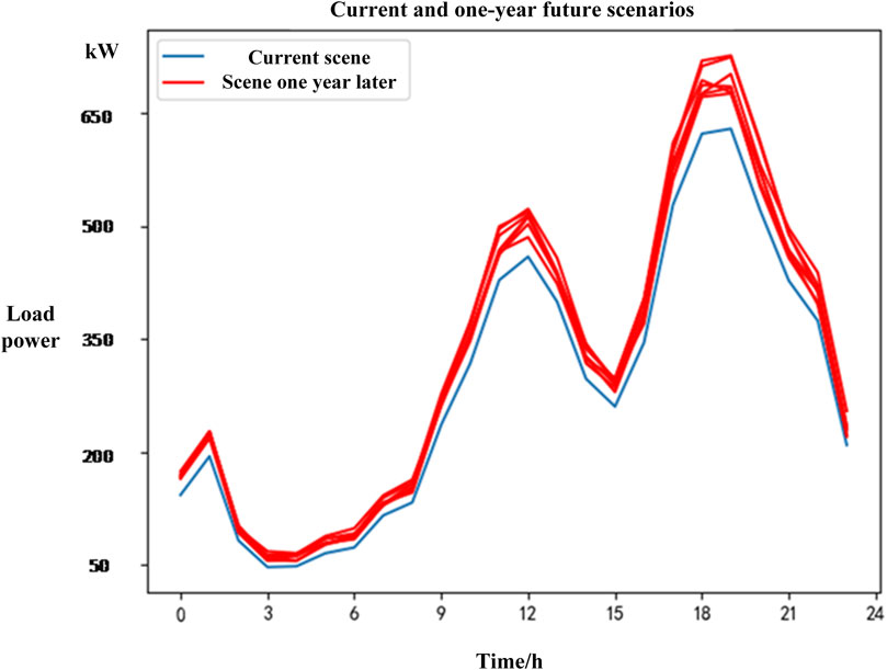
Figure 9. Planning-stage daily load operation scenario for a certain distribution area after 1 year.

Figure 10

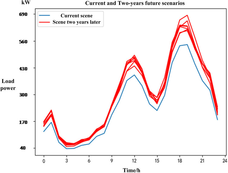
Figure 10. Planning-stage daily load operation scenario for a certain distribution area after 2 years.

From Figures 9, 10, it can be seen that with social development and improvement in people’s living standards, the load connected to a certain transformer area in the distribution network gradually increases. For a given day-ahead load scenario, through the study and calculation of the load growth pattern, the possible load scenarios after 1 year and 2 years are shown by the red lines in Figures 9, 10, respectively, representing the planning-stage daily load operation scenarios for this distribution area.

2.3 Typical weather day classification considering meteorological factor distribution characteristics

The natural correlation between PV output and meteorological information means that different meteorological data corresponds to different PV output scenarios. These meteorological factors mainly include solar radiation, temperature, precipitation, and wind speed. Based on the factors that significantly influence PV output and load power, regional weather is classified into several typical weather days. However, selecting more meteorological features is not always better. The correlation between PV output time series and meteorological features, as well as between load power and meteorological features, can be analyzed separately to select highly correlated meteorological features as the basis for dataset division.

2.3.1 Correlation analysis of meteorological features and sample data based on spearman correlation

Spearman correlation coefficient is a non-parametric measure of rank correlation, which can effectively measure the strength of the monotonic relationship between two variables (Su, 2023). For the relationship between PV output and meteorological features, the Spearman correlation coefficient ranks both the meteorological feature values and PV output sample data values from smallest to largest, calculating correlation using these ranks rather than actual values (Li, 2023).

To complete the correlation analysis between meteorological features and PV output/load power, this paper selects the Spearman correlation coefficient to analyze the correlation between six sample meteorological features (radiation, air pressure, relative humidity, precipitation, temperature, and sunshine duration) and PV output/load power sample data. The specific formula is shown in Equation 17:

$\mathrm{\rho }=\frac{{\displaystyle {\sum }_{\mathrm{i}=1}^{\mathrm{N}}}\left({\mathrm{x}}_{\mathrm{i}}-\overline{\mathrm{x}}\right)\left({\mathrm{y}}_{\mathrm{i}}-\overline{\mathrm{y}}\right)}{\sqrt{{\displaystyle {\sum }_{\mathrm{i}=1}^{\mathrm{N}}}{\left({\mathrm{x}}_{\mathrm{i}}-\overline{\mathrm{x}}\right)}^2{\left({\mathrm{y}}_{\mathrm{i}}-\overline{\mathrm{y}}\right)}^2}}(17)$

Where: N is the number of processed PV output sample data or meteorological sample data, ${\mathrm{x}}_{\mathrm{i}}$ and ${\mathrm{y}}_{\mathrm{i}}$ are the i-th sample PV output value and i-th sample weather feature value respectively, and are the average values of sample PV output and sample weather features respectively.

Through the calculation of Equation 17, the correlation coefficients between the six sample meteorological features and PV output/load power sample data are obtained, denoted as. The results are shown in Table 3.

Table 3

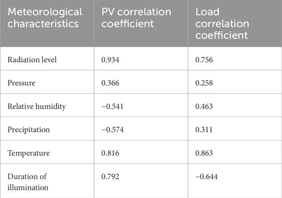
Table 3. Correlation analysis results of meteorological features with PV and load.

From the PV correlation coefficient column in Table 3, it can be seen that radiation, temperature, and sunshine duration have high correlations with PV output, with radiation having the highest correlation coefficient. The load correlation coefficient column shows that load power is also highly correlated with these three meteorological features, with temperature having the highest correlation coefficient with load power. Therefore, these three meteorological factors can be selected as the classification standard for typical weather days in this region for studying PV output and load power.

2.3.2 Typical weather day dataset division

Due to differences in climatic conditions across regions, mechanically dividing historical PV and load data into four seasonal datasets lacks applicability. Considering that meteorological conditions in the same area are stable over long time scales, generally alternating between specific types of weather days, and the proportion of a certain typical weather day in an annual meteorological cycle doesn't change significantly. To avoid mechanically using the average or median of meteorological factors as the division standard, this paper uses kernel density estimation to visualize the distribution characteristics of each meteorological factor and completes the division based on the distribution characteristics of regional meteorological factors. The data used in this paper’s case study is from a regional distribution network in Guangdong for the entire year of 2022. The specific division process is as follows:

(1) Select temperature, radiation, and sunshine duration as meteorological conditions for dataset division;

(2) For temperature, calculate the average daily temperature from the dataset, obtain the daily average temperature dataset, and use kernel density estimation to fit its distribution characteristics, as shown in Figure 11. Based on the distribution characteristics of daily average temperature, 19.2°C can be set as the temperature division point. For the i-th day, if the daily average temperature is higher than 19.2°C, it is considered a high-temperature day, otherwise a low-temperature day. Mark high-temperature days as 1 and low-temperature days as 0;

(3) For radiation, calculate the average daily radiation from the dataset, obtain the daily average radiation dataset, and use kernel density estimation to fit its distribution characteristics, as shown in Figure 12. Based on the distribution characteristics of daily average radiation, 147.4W/m² can be set as the radiation division point. For the i-th day, if the daily average radiation is higher than 147.4W/m², it is considered a high-radiation day, otherwise a low-radiation day. Mark high-radiation days as 1 and low-radiation days as 0;

(4) For light intensity (measured in Lux), count the number of hours in a day when the average light intensity within an hour is greater than 800 Lux, considering that hour to be in a bright state. After calculation, use a bar chart to represent the frequency of daily sunshine hours in the dataset, as shown in Figure 13. Based on the bar chart, 9 h can be set as the division point for sunshine duration. For the i-th day, if its sunshine duration is greater than or equal to 9 h, it is considered a long sunshine day, otherwise a short sunshine day. Mark long sunshine days as 1 and short sunshine days as 0;

(5) Based on the meteorological conditions from steps 2), 3), and 4), the dataset can be divided into 2 × 2 × 2 = 8 specific weather day types, forming the matrix in Equation 18:

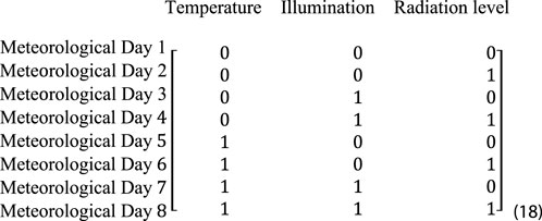
(6) According to the dates corresponding to each data category in the matrix, divide the distribution network area into 8 weather day types, and extract the corresponding PV and load data for each date. If the data for a certain category is extremely scarce, merge it with a similar category’s dataset. Finally, obtain 8 weather day dataset divisions based on the distribution characteristics of meteorological factors.

Figure 11

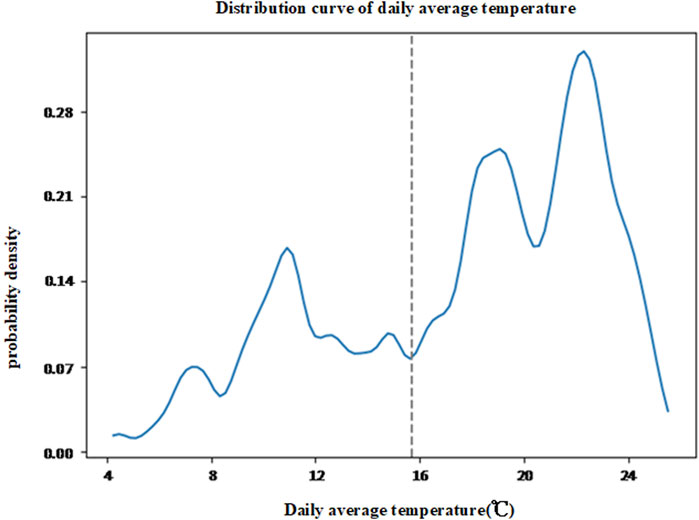
Figure 11. Distribution of daily average temperature.

Figure 12

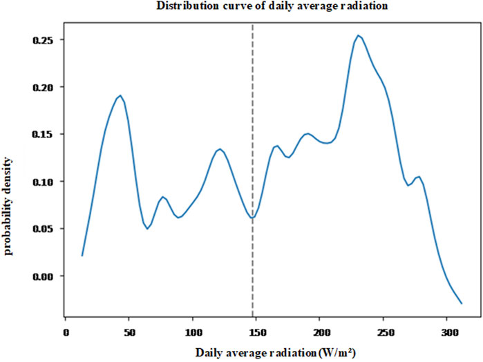
Figure 12. Distribution of daily average radiation.

Figure 13

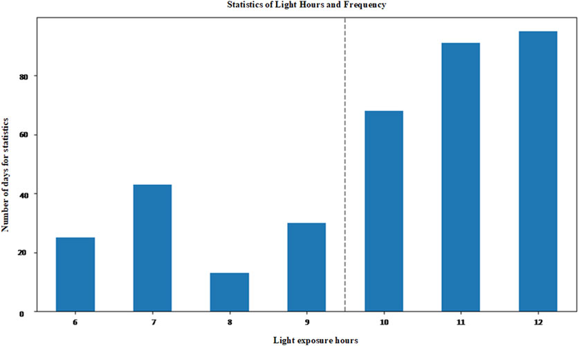
Figure 13. Frequency statistics of sunshine hours.

After constructing a large number of planning-stage PV and load daily scenario description matrices, divide the planning-stage PV and load daily scenario data into 8 different typical weather day datasets according to the dates of weather days, forming 8 planning-stage PV output datasets and 8 planning-stage load power datasets.

The following is the dataset classification of planning-stage PV and load scenarios for a feeder line with rooftop PV integration in Guangdong area for 2021 and 2022. The study period is two consecutive full years, i.e., 730 daily operation scenarios each for PV and load. According to the local typical weather day division method, these 730 daily operation scenarios are divided (Chong et al., 2023), and the classification results are shown in Table 4:

Table 4

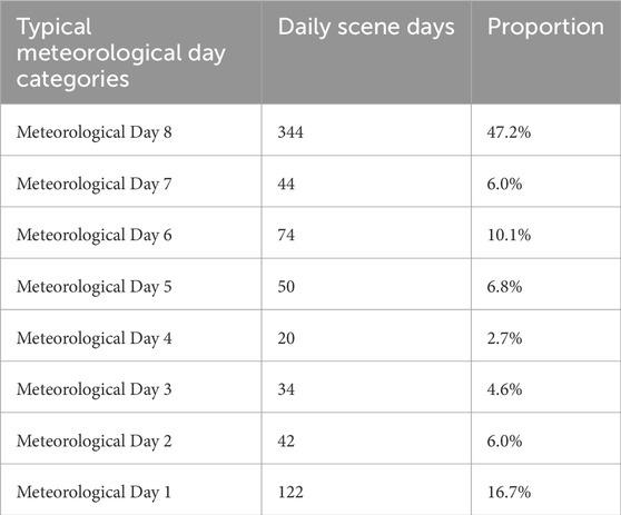
Table 4. Typical weather day dataset division.

3 Experimental results and related discussions

3.1 Scenario generation and validation

Due to the large number of historical operational scenarios involving photovoltaic systems and loads in the distribution network, it is necessary to perform scenario reduction to derive a limited number of representative historical scenarios. Scenario reduction employs mathematical algorithms and analysis to reduce the number of similar scenarios during the study period, thus lowering computational complexity (Qun et al., 2023). In this paper, the k-means clustering algorithm is used to perform scenario reduction on the 16 datasets mentioned above, utilizing Euclidean distance to measure the distance between data points. This ensures that scenarios within the same cluster have significant similarities, while those in different clusters display distinct differences (Li et al., 2023). This is particularly appropriate for the photovoltaic and load power curves. Ultimately, the cluster centers of each cluster are used as the typical scenarios for each typical meteorological day dataset.

The steps of the clustering algorithm are as follows:

1) Randomly select a data point from the dataset as the first cluster center $K_1$.

2) Calculate the distance between other sample data and the initial cluster center $K_1$, and select the sample data farthest away as the new center $K_2$.

3) For the i-th cluster center ${\mathrm{K}}_{\mathrm{i}}\left(\mathrm{i}\ge 3\right)$, it should satisfy the condition $\mathit{max}\left\{\mathit{min}\left({\mathrm{d}}_{\mathrm{i},1},{\mathrm{d}}_{\mathrm{i},2},...,{\mathrm{d}}_{\mathrm{i}-1,\mathrm{M}}\right)\right\}$ where ${\mathrm{d}}_{\mathrm{i}-1,\mathrm{M}}$ is the distance between the $\left(\mathrm{i}-1\right)-\text{th}$ cluster center and the M-th group of data.

4) Repeat step 3) until K cluster centers have been selected.

5) Assign all data points to the nearest cluster center.

6) Recalculate the cluster centers based on the data points in each cluster.

7) Repeat steps 5) and 6) until the cluster centers no longer change or a predefined number of iterations is reached.

To determine the optimal number of clusters for each scenario set, the Elbow Method is used in step 4) to identify the best number of clusters. The basic principle of this method is to observe the relationship between the sum of squared errors (SSE) and the number of clusters, looking for an inflection point or elbow, where the corresponding number of clusters is deemed optimal (Yuan and Yang, 2019). This completes the generation of typical historical scenarios for each specific meteorological day.

Figure 14 shows the cluster centers obtained using the k-means clustering method for 344 load and photovoltaic daily scenarios under meteorological day 8 at nodes 7/12, with three centers for load and two for photovoltaic. Figure 15 shows the typical scenarios corresponding to these cluster centers.

Figure 14

Figure 14. Clustering results of load and photovoltaic data at node 7/12 and meteorological day 8.

Figure 15

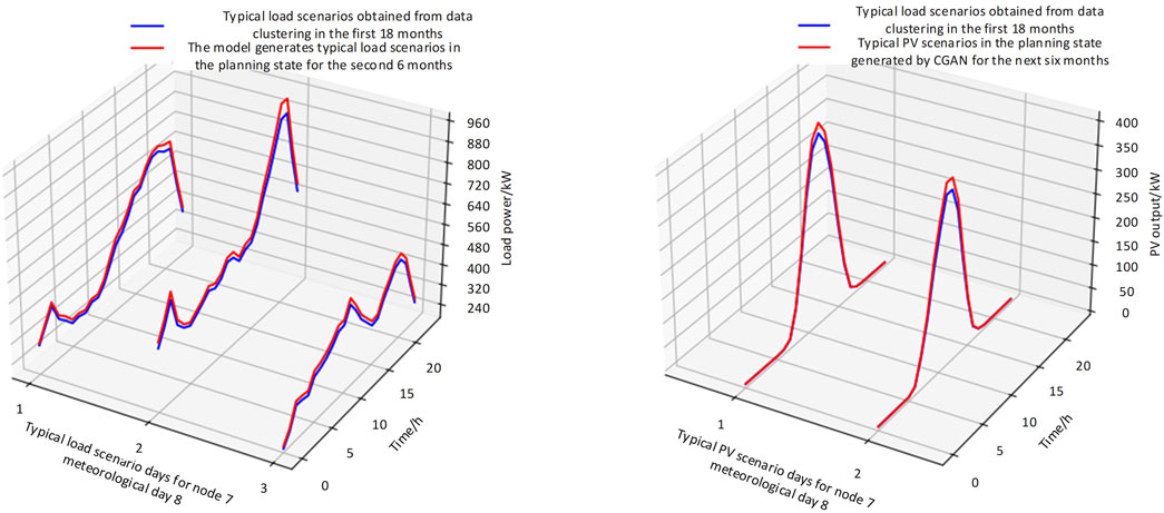
Figure 15. Typical daily scenarios of load and photovoltaic under node 7/12, meteorological day 8.

In addition, clustering analysis was conducted on each meteorological day dataset, and the clustering results are shown in Table 5.

Table 5

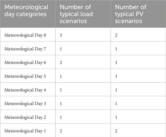
Table 5. Number of load and typical photovoltaic scenarios on each meteorological day.

Meteorological day division method discussed in this paper, the number of typical scenarios can be reduced to 12 for load nodes and 10 for photovoltaic nodes. In practice, these 22 typical scenarios do not appear randomly but are manifested according to the division of meteorological days, aligning with specific photovoltaic-load day scenarios within those days.

3.2 Practical application and computational efficiency

The proposed mathematical models and algorithms are designed to be applicable to real-world distribution networks. The Conditional Generative Adversarial Network (CGAN) and Bass model are implemented in a modular fashion, allowing for easy integration with existing distribution network planning tools. For instance, the CGAN can be trained offline using historical PV and load data, and the trained model can then be deployed to generate scenarios for specific future time horizons. This approach minimizes the computational burden during real-time planning, as the scenario generation process is decoupled from the optimization of network configurations.

Regarding computational complexity, the CGAN training process is the most resource-intensive step, as it involves iterative updates of the generator and discriminator networks. However, once trained, the CGAN can generate scenarios in a matter of seconds, making it highly efficient for practical applications. The Bass model, which is used to estimate future PV capacity, is computationally lightweight and can be executed in real-time. The overall computational efficiency of our method is further enhanced by the use of k-means clustering for scenario reduction, which reduces the number of scenarios to a manageable size without significant loss of information.

For large-scale networks, the proposed method can be scaled by parallelizing the CGAN training process and distributing the scenario generation across multiple computing nodes. Additionally, the modular design of the algorithm allows for integration with existing software tools, such as distribution network simulators and optimization platforms, enabling seamless implementation in real-world planning workflows. The experimental results demonstrate that the proposed method achieves a balance between computational efficiency and scenario accuracy, making it a practical tool for distribution network planning.

3.3 Dynamic characteristics of PV generation and scenario realism

The proposed CGAN model captures short-term PV variability by learning temporal correlations in historical data, enabling realistic hourly PV output scenarios. For example, it replicates rapid fluctuations caused by weather changes, as shown in the generated scenarios for nodes 7/12 (see Figures 6, 7). Combined with the Bass model, which estimates future PV capacity growth, the framework accounts for long-term trends and seasonal variations, ensuring scenarios reflect both short-term and long-term dynamics.

By classifying typical weather days based on radiation, temperature, and sunshine duration, the model inherently captures seasonal and weather-driven PV variability. This enhances scenario realism, as demonstrated in the clustering results for meteorological day 8 (see Figures 14, 15). While the current model does not explicitly use advanced time-series techniques, its modular design allows future integration of detailed meteorological data or seasonal forecasting models, further improving applicability to real-world planning.

4 Discussion

4.1 Experimental validation and comparative analysis

The example feeder line in this article is a 10 kV feeder line located in a certain area of Guangdong. Its topology structure is shown in Figure 2, and the photovoltaic, load, and meteorological data are the operational data of the feeder line for the years 2021 and 2022. In order to highlight the advantages of the planning state typical scenario construction method considering specific meteorological days in this article, we compared the photovoltaic and load scenarios under 8 meteorological days in the example feeder line, using the planning state typical scenario construction method considering specific meteorological days in this article and the typical scenario generation method using only historical data to reasonably superimpose photovoltaic and load growth rates. The scenario reduction was achieved using k-means clustering method.

For the validation method in this article, the photovoltaic and load data of the node for the first 18 months before 7/12 are shown below as training data for CGAN. Combined with the Bass model prediction results and clustering algorithm, a typical planning scenario for the next 6 months is constructed. For the method of considering only historical data and reasonably adding growth rates, the annual average photovoltaic and load growth rates are calculated using the photovoltaic and load data before 2022, and then the growth rates are reasonably added based on the operating data of the first half of 2022 to form the predicted photovoltaic and load operating data for the second half of 2022. Compare the scenarios generated by the above two methods with typical operating scenarios in the second half of 2022. The average errors of load and photovoltaic scenarios are shown in Figures 16, 17, respectively.

Figure 16

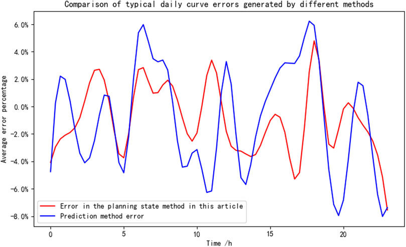
Figure 16. Comparison of errors in node 7/12 load scenarios under different methods.

Figure 17

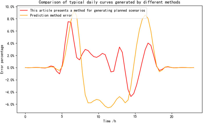
Figure 17. Comparison of node 7/12 photovoltaic scene error under different methods.

Analysis of the results from Figure 17 and Figure 18 reveals that, compared to the method that generates future load and photovoltaic scenarios solely based on historical load data, the planning state load and photovoltaic scenario construction method proposed in this paper is more aligned with real-world conditions. This is because the planning state scenario generation method developed in this study extensively investigates each load node type and its growth characteristics, as well as the probability of new capacity at each photovoltaic node. Consequently, for distribution networks rapidly integrating rooftop photovoltaics, the method presented in this paper offers a higher degree of accuracy in generating planning state load and photovoltaic scenarios.

4.2 Methodological advantages and practical applicability

The proposed methodology is designed with practical application in mind, particularly for real-world distribution networks. The Conditional Generative Adversarial Network (CGAN) and Bass model are implemented in a modular fashion, enabling seamless integration with existing distribution network planning tools. For instance, the CGAN can be trained offline using historical PV and load data, and the trained model can generate scenarios for specific future time horizons in a matter of seconds. This decouples the scenario generation process from real-time optimization, significantly reducing computational burden during planning tasks. The Bass model, used for estimating future PV capacity, is computationally lightweight and can be executed in real-time, further enhancing the method’s efficiency.

For large-scale networks, the scalability of our approach is ensured by the parallelizability of the CGAN-based scenario generation process. Scenarios for different nodes or time horizons can be generated independently, allowing the method to be efficiently scaled using distributed computing resources. Additionally, the modular design of the algorithm facilitates its integration with widely used optimization platforms such as MATPOWER and OpenDSS, making it suitable for real-world planning workflows.

4.3 Scenario generation rigor and validation

Regarding the scenario generation process, we employ a rigorous methodology to ensure the accuracy and representativeness of the generated scenarios. Historical PV and load data are preprocessed and used to train the CGAN, which learns the underlying distribution of PV output and load demand under varying meteorological conditions. Typical scenarios are selected using the k-means clustering algorithm, with cluster centers chosen as representative scenarios. The number of clusters is determined using the Elbow Method, balancing representativeness and computational efficiency.

To validate the accuracy of the generated scenarios, we compare them with historical operating data, calculating metrics such as mean absolute error (MAE) and root mean square error (RMSE). As shown in Figures 16, 17, the generated scenarios exhibit low error rates, confirming their alignment with real-world conditions. This validation process ensures that the scenarios are not only representative but also reliable for use in distribution network planning.

4.4 Limitations and future refinements

The Bass model simplifies the diffusion process by assuming homogeneous user behavior and static innovation/imitation coefficients (Mahajan et al., 1990). However, this approach may overlook regional economic disparities or policy-driven incentives that influence rooftop PV adoption rates. For example, Tsoularis and Wallace (2002) proposed a phased logistic growth model to capture heterogeneous diffusion dynamics across sub-regions (Tsoularis and Wallace, 2002). Future enhancements could incorporate multi-scale modeling, such as fitting region-specific Bass parameters or embedding stochastic processes, to improve prediction accuracy in heterogeneous markets. Additionally, high-resolution data on user demographics and policy impacts could enable discrimination among competing diffusion models for tailored planning.

While the proposed CGAN and Bass model framework effectively leverages historical data to generate planning-stage scenarios, it is essential to acknowledge its limitations in anticipating technological innovations. For instance, breakthroughs in photovoltaic materials or energy storage systems may significantly alter future energy landscapes, which cannot be fully captured by historical data alone. As noted by Norton and Bass (1987), successive generations of technology can disrupt traditional diffusion patterns, leading to deviations in market penetration predictions. To address this, future research could integrate technology trend forecasting or dynamic parameter adjustments into the model to better account for uncertainties arising from disruptive innovations.

4.5 Summary of contributions

In summary, our method addresses key challenges in scenario generation for distribution networks, offering a computationally efficient and scalable solution that can be readily integrated into existing planning workflows. The validation results further underscore the practical applicability and accuracy of the generated scenarios, making our approach a valuable tool for addressing the complexities of high-penetration PV integration and load growth in modern distribution networks.

5 Conclusion

1) For distribution networks rapidly integrating rooftop photovoltaics, this paper adopts a method driven by historical data using Conditional Generative Adversarial Networks (CGANs). It innovatively captures the photovoltaic capacity and three meteorological factors that have the highest correlation with photovoltaic output, thus generating planning state photovoltaic output scenarios for specific meteorological days and capacities. This approach addresses the limitations of traditional methods that rely solely on historical photovoltaic data for future scenario generation.

2) Regarding the correlation between meteorological factors and both load and photovoltaic outputs, this study employs the Spearman correlation coefficient method to analyze the correlation between meteorological characteristics and sample data. It identifies the three meteorological factors that have the highest correlation with load and photovoltaic outputs. Considering the unique meteorological distribution characteristics of each region, this paper avoids mechanically using the mean or median values of meteorological factors as classification standards. Instead, it employs kernel density estimation to visualize the distribution characteristics of each meteorological factor, allowing for the segmentation of meteorological factors based on variable quantiles according to regional characteristics.

3) Concerning the integration of planning state photovoltaic-load typical scenarios, this paper avoids mechanically dividing historical photovoltaic and load data into four seasonal datasets. Given that meteorological conditions in the same region are stable over long time scales and typically only a few specific meteorological days alternate, and that the proportion of a particular type of meteorological day does not vary significantly over an annual cycle, this study innovatively classifies future meteorological days using the meteorological factors most correlated with load and photovoltaic outputs. Therefore, the few planning state typical photovoltaic-load scenarios generated can be effectively combined under corresponding typical meteorological days.

6 Future work

The current methodology focuses on single-region distribution network planning. However, real-world power systems require coordinated multi-regional renewable energy deployment to mitigate generation volatility. Facchini et al. (2021) demonstrated that leveraging meteorological correlations across regions can optimize resource allocation and reduce fluctuations (Facchini et al., 2021). Furthermore, policy interventions—such as feed-in tariffs or renewable portfolio standards—could regulate the ‘natural penetration’ modeled by Bass curves, ensuring grid stability (Surmonte et al., 2021). Future work will explore correlated weather scenario generation for geographically dispersed systems and develop policy-aware Bass models to support national-scale energy planning. Stochastic approaches, as proposed by Scala et al. (2019), could further enhance robustness by integrating uncertainty in weather patterns and policy enforcement.

Data availability statement

The data analyzed in this study is subject to the following licenses/restrictions: Due to local legal reasons, the dataset cannot be directly made public. Requests to access these datasets should be directed to Xixian Liu, MjExMjIwNDUxMUBtYWlsMi5nZHV0LmVkdS5jbg==.

Author contributions

CG: Conceptualization, Data curation, Formal Analysis, Investigation, Methodology, Project administration, Software, Validation, Visualization, Writing–original draft, Writing–review and editing. QL: Conceptualization, Funding acquisition, Investigation, Methodology, Validation, Writing–original draft, Writing–review and editing. PC: Software, Validation, Writing–review and editing. ZX: Formal Analysis, Writing–review and editing. XW: Investigation, Visualization, Writing–review and editing. XL: Resources, Supervision, Writing–review and editing. FZ: Data curation, Writing–original draft, Writing–review and editing.

Funding

The author(s) declare that financial support was received for the research, authorship, and/or publication of this article. This research was supported by the planning subject project of Guangdong Power Grid Power Grid Co Ltd (031000QQ00240009). The funder was not involved in the study design, collection, analysis, interpretation of data, the writing of this article, or the decision to submit it for publication.

Conflict of interest

Authors CG, QL, PC, ZX, and XW were employed by Department of Distribution Network Planning and Research Planning Research of Guangdong Power Grid Co., Ltd.

The remaining authors declare that the research was conducted in the absence of any commercial or financial relationships that could be construed as a potential conflict of interest.

Publisher’s note

All claims expressed in this article are solely those of the authors and do not necessarily represent those of their affiliated organizations, or those of the publisher, the editors and the reviewers. Any product that may be evaluated in this article, or claim that may be made by its manufacturer, is not guaranteed or endorsed by the publisher.

References

Ali, E., and Qiang, Y. (2019). State-of-the-art techniques for modelling of uncertainties in active distribution network planning: a review. Appl. energy 239 1509–1523. doi:10.1016/j.apenergy.2019.01.211

CrossRef Full Text | Google Scholar

Chen, H., Jiang, W., and Han, J. (2021). Research on typical scenario generation method for photovoltaic power stations considering output power correlation. Electr. Power Eng. Technol. 40 (02), 11–17+25.

Google Scholar

Cheng, L., Liu, G., Huang, H., Wang, X., Chen, Y., and Zhang, J. (2020). Equilibrium analysis of general N-population multi-strategy games for generation-side long-term bidding: an evolutionary game perspective. J. Clean. Prod. doi:10.1016/j.ijepes.2020.106743

CrossRef Full Text | Google Scholar

Cheng, L., Peng, P., Lu, W., Huang, P., and Chen, Y. (2024). Study of flexibility transformation in thermal power enterprises under multi-factor drivers: application of complex-network evolutionary game theory. Mathematics doi:10.3390/math12162537

CrossRef Full Text | Google Scholar

Cheng, L., Yin, L., Wang, J., Shen, T., Chen, Y., Liu, G., et al. (2021). Behavioral decision-making in power demand-side response management: a multi-population evolutionary game dynamics perspective. Int. J. Electr. Power and Energy Syst. 129, 106743–0142-0615. doi:10.1016/j.ijepes.2020.106743

CrossRef Full Text | Google Scholar

Chong, G., Peng, Z., Qiang, L., Yao, D., Ye, H., Ran, C., et al. (2023). Evaluation method of distribution network power supply capacity considering actual load growth pattern. South. Power Syst. Technol. 17(07), 115–124. doi:10.13648/j.cnki.issn1674-0629.2023.07.013

CrossRef Full Text | Google Scholar

Colmenar-Santos, A., Reino-Rio, C., Borge-Diez, D., and Collado-Fernández, E. (2016). Distributed generation: a review of factors that can contribute most to achieve a scenario of DG units embedded in the new distribution networks. Renew. Sustain. Energy Rev. 59, 1130–1148. doi:10.1016/j.rser.2016.01.023

CrossRef Full Text | Google Scholar

Ehsanbakhsh, M., and Sepasian, M. S. (2023). Bi-objective robust planning model for optimal allocation of soft open points in active distribution network: a flexibility improvement approach. Electr. Power Syst. Res. 224, 109780. doi:10.1016/j.epsr.2023.109780

CrossRef Full Text | Google Scholar

Facchini, A., and Scala, A. (2021). “Complex systems applications to electric mobility and regional intermittent source planning.” in Renewable energy integration (Academic Press), 641–664.

Google Scholar

Gao, Y., Hu, X., Yang, W., Liang, H., and Li, P. (2017). Multi-objective bilevel coordinated planning of distributed generation and distribution network frame based on multiscenario technique considering timing characteristics, IEEE Trans. Sustain. Energy, 8(4), 1415–1429. doi:10.1109/TSTE.2017.2680462

CrossRef Full Text | Google Scholar

Goodfellow, I., Pouget-Abadie, J., Mirza, M., Xu, B., Warde-Farley, D., Ozair, S., et al. (2014a). Generative adversarial nets. Adv. Neural Inf. Process. Syst. 27. doi:10.48550/arXiv.1406.2661

CrossRef Full Text | Google Scholar

Goodfellow, I. J., Pouget-Abadie, J., Mirza, M., Xu, B., Warde-Farley, D., Ozair, S., et al. (2014b). “Generative adversarial nets.” in International conference on neural information processing systems.

Google Scholar

He, M., Soltani, Z., Khorsand, M., Dock, A., Malaty, P., and Esmaili, M. (2022). Behavior-aware aggregation of distributed energy resources for risk-aware operational scheduling of distribution systems. Energies 15, 9420. doi:10.3390/en15249420

CrossRef Full Text | Google Scholar

Hu, J., and Li, H. (2022). A transfer learning-based scenario generation method for stochastic optimal scheduling of microgrid with newly-built wind farm. Renew. Energy 185, 1139–1151. doi:10.1016/j.renene.2021.12.110

CrossRef Full Text | Google Scholar

Hu, S., Zhu, R., and Tang, B. (2022). WGAN photovoltaic power scenario generation method with gradient penalty. J. Electr. Power Syst. Automation 34 (11), 109–115. doi:10.19635/j.cnki.csu-epsa.000993

CrossRef Full Text | Google Scholar

Jun, D., Rui, L., Shuchun, H., Kun, L., and Zhuang, L. (2023). Short-term power generation forecast of distributed photovoltaic based on BIRCH clustering and L-Transformer. High. Volt. Eng. 1-14. doi:10.13336/j.1003-6520.hve.20230809

CrossRef Full Text | Google Scholar

Lefeng, C., Yang, C., and Guiyun, L. (2022). 2PnS-EG: a general two-population n-strategy evolutionary game for strategic long-term bidding in a deregulated market under different market clearing mechanisms. doi:10.1016/j.ijepes.2022.108182

CrossRef Full Text | Google Scholar

Li, Y., Liu, Y., and Feng, L. (2023). Feature extraction and fault detection of nonlinear dynamic process based on Spearman correlation analysis. J. Shandong Univ. Sci. Technol. Nat. Sci. Ed. 42 (02), 98–107. doi:10.16452/j.cnki.sdkjzk.2023.02.011

CrossRef Full Text | Google Scholar

Li, Z. (2023). Research on charging station planning based on electric vehicle quantity prediction. J. Taiyuan Urban Vocat. Coll. (12), 32–36. doi:10.16227/j.cnki.tycs.2023.0687

CrossRef Full Text | Google Scholar

Mahajan, V., Muller, E., and Bass, F. M. (1990). New product diffusion models in marketing: a review and directions for research. J. Mark. 54 (1), 1–26. doi:10.1177/002224299005400101

CrossRef Full Text | Google Scholar

Niu, G., Ji, Y., Zhang, Z., Wang, W., Chen, J., and Yu, P. (2021). Clustering analysis of typical scenarios of island power supply system by using cohesive hierarchical clustering based K-Means clustering method. Energy Rep. 7:250–256. doi:10.1016/j.egyr.2021.08.049

CrossRef Full Text | Google Scholar

Norton, J. A., and Bass, F. M. (1987). A diffusion theory model of adoption and substitution for successive generations of high-technology products. Manag. Sci. 33 (9), 1069–1086. doi:10.1287/mnsc.33.9.1069

CrossRef Full Text | Google Scholar

Qun, Y., Xiaodong, H., Jian, H., Lin, L., Jianxin, Z., and Yuyao, F. (2023). Trend prediction of power outages in China's power grid based on Spearman correlation coefficient and system inertia. Proc. Chin. Soc. Electr. Eng. 43(14), 5372–5381. doi:10.13334/j.0258-8013.pcsee.220035

CrossRef Full Text | Google Scholar

Scala, A., Facchini, A., Perna, U., and Basosi, R. (2019). Portfolio analysis and geographical allocation of renewable sources: a stochastic approach. Energy Policy 125, 154–159. doi:10.1016/j.enpol.2018.10.034

CrossRef Full Text | Google Scholar

Su, H. (2023). Research on the carrying capacity assessment of distribution network considering distributed rooftop photovoltaic access. Doctoral dissertation, Guangdong University of Technology. Available online at: https://d.wanfangdata.com.cn/thesis/ChhUaGVzaXNOZXdTMjAyNDA5MjAxNTE3MjUSCUQwMzExNjcwMBoIbHFrZHl3ZDQ%3D

Google Scholar

Surmonte, F., Perna, U., Scala, A., Rubino, A., and Facchini, A. (2021). A data-driven approach to renewable energy source planning at regional level. Energy Sources, Part B Econ. Plan. Policy 16 (1), 1064–1075. doi:10.1080/15567249.2021.1926598

CrossRef Full Text | Google Scholar

Tsoularis, A., and Wallace, J. (2002). Analysis of logistic growth models. Math. Biosci. 179 (1), 21–55. doi:10.1016/s0025-5564(02)00096-2

PubMed Abstract | CrossRef Full Text | Google Scholar

Uddin, M., Mo, H., Dong, D., Elsawah, S., Zhu, J., and Guerrero, J. M. (2023). Microgrids: a review, outstanding issues and future trends. Energy Strategy Rev. 49, 101127. doi:10.1016/j.esr.2023.101127

CrossRef Full Text | Google Scholar

Wang, X., Zhong, F., Xu, Y., Liu, X., Li, Z., Liu, J., et al. (2023). Extraction and joint method of PV–load typical scenes considering temporal and spatial distribution characteristics. Energies 16(18), 6458. doi:10.3390/en16186458

CrossRef Full Text | Google Scholar

Wenlong, L., Dechang, Y., Leijiao, G., Zhe, Y., Kuangpu, L., and Runan, S.(2022). Renewable energy scenario generation based on pixel convolutional generative network. High. Volt. Eng. 48(04), 1320–1331. doi:10.13336/j.1003-6520.hve.20211721

CrossRef Full Text | Google Scholar

Yang, H., Liang, R., Yuan, Y., Chen, B., Xiang, S., Liu, J., et al. (2022). Distributionally robust optimal dispatch in the power system with high penetration of wind power based on net load fluctuation data. Appl. Energy 313, 118813. doi:10.1016/j.apenergy.2022.118813

CrossRef Full Text | Google Scholar

Yanping, W., Jun, W., Nanfan, L., and Zhangli, S. (2023). Multi-scenario prediction model of random power in parks based on Markov chain. Integr. Intell. Energy 45 (01), 14–22.

Google Scholar

Yuan, C., and Yang, H. (2019). Research on K-value selection method of K-means clustering algorithm. J 2, 226–235. doi:10.3390/j2020016

CrossRef Full Text | Google Scholar

Zhangjin, F., Jun, X., Fengmei, L., Xinying, X., and Junjie, D. (2021). Research on a magnetic tile defect image generation method based on improved DCGANs network. Mini-Micro Comput. Syst. 42(03), 589–594.

Google Scholar

Zhang, S., Cheng, H., Wang, D., Zhang, L., Li, F., and Yao, L. (2018). Distributed generation planning in active distribution network considering demand side management and network reconfiguration. Appl. Energy 228, 1921–1936. doi:10.1016/j.apenergy.2018.07.054

CrossRef Full Text | Google Scholar

Zhu, Z., Cheng, L., and Shen, T. (2024). Spontaneous formation of evolutionary game strategies for long-term carbon emission reduction based on low-carbon trading mechanism. Mathematics 12 (19), 3109. doi:10.3390/math12193109

CrossRef Full Text | Google Scholar