Analysis of transient characteristics and fault ride-through control of hybrid grid-tied converters with grid-following and grid-forming

When the Grid-Following (GFL) and the Grid-Forming (GFM) converters are hybrid-connected to the grid, they are coupled through the grid impedance. During grid faults, the transient characteristics of the two converters become more complex due to this coupling. If one of the converters experiences stability issues, it affects the other, making fault ride-through challenging. A mathematical model for the hybrid grid-connected system of the two converters is first established to analyze the existence conditions of the equilibrium point. Using the phase-plane method, the mutual influence mechanism during faults is revealed. Subsequently, a method to adjust the GFM phase angle based on the degree of voltage sag is proposed, which also improves the phase-locked loop (PLL) of the GFL. The influence of GFL current injection is considered to limit the GFM fault current, thereby achieving hybrid fault ride-through control. Finally, the simulation verifies the effectiveness of the proposed control strategy. The results show that the proposed method can adjust the phase angle to support the grid, ensuring that the GFM outputs more reactive current within the maximum allowable current range. Meanwhile, the GFL injects current according to grid guidelines, effectively preventing overcurrent and phase angle instability of the converters.

1 Introduction

With the implementation of carbon peaking and carbon neutrality policies, the development and application of renewable energy have progressively become essential pathways toward achieving green, low-carbon, and sustainable development goals (Huang et al., 2024). The share of non-synchronous generation in power systems is steadily increasing, resulting in high proportions of renewable energy and power electronic devices becoming defining features of modern power systems (Gu and Green, 2023). A high proportion of new energy and power electronic equipment has become a notable characteristic of power systems. In order to provide the system support, a serial of the control is implemented into the Inverter-Based Resources (IBR). In general, the control of the IBR can be classified into the GFL and GFM. It is worth noting that using GFL as the main grid - connected devices does not provide sufficient inertia and damping for the system, resulting in a further decrease in system inertia, which jeopardizes the safe operation of the power system. GFM, which possess the characteristics of a synchronous generator, have garnered widespread attention. Compared to GFL, they can effectively function as a voltage source, allowing them to regulate system voltage and frequency and provide necessary inertia and damping support. Nevertheless, GFL still have advantages that GFM cannot replace. On the other hand, the current new energy power stations are equipped with GFL, making it impractical to replace them all with GFM. Therefore, a feasible alternative is to modify some of the already installed converters to grid-forming control. This implies that in future power systems, both grid-following and GFM will coexist (Zhao and Flynn, 2022).

Both GFL and GFM converters achieve frequency and voltage support functions. However, due to their different roles in the power system, their transient responses will also differ (Wei et al., 2024). The GFL behaves as a controlled current source, which uses the PLL to detect the grid state on the frequency and voltage and then accordingly provides a passive support (Kim et al., 2024). While the GFM behaves as a controlled voltage source, of which mechanism is similar with the power-angle transients of the synchronous generator and thus, which naturally can provide an active support (Zhang et al., 2023). In the event of a grid fault, a synchronous generator can inject 6 to 8 times its rated current (pu) to support the grid (Taul et al., 2020). However, the overcurrent tolerance of converters is relatively low. Without proper control, this could lead to disconnection of renewable energy generation equipment from the grid or damage to the converters. To address this, IEEE standard 2,800–2022 provides detailed technical requirements for renewable energy generation equipment regarding fault ride-through capabilities (IEEE, 2022). Currently, research mainly focuses on the transient processes of single GFL or single GFM converters during fault ride-through, with an emphasis on the control of fault current and power angle. For GFL, Zhang and Schuerhuber (2023) enhances system stability during grid faults and improves post-fault recovery performance by adjusting current injection via PLL frequency feedback. However, the steady-state operating points and stability become challenging to predict. Xu et al. (2021), by removing the frequency feedback loop and employing frequency-locking techniques, fixes the PLL frequency to maintain its output at the state of the previous moment. Nonetheless, this approach struggles to meet the requirements of grid codes. He et al. (2021) suggests locking only the integral part of the PLL during faults, but this method fails when there is no equilibrium point after the fault. Gao et al. (2023) adjusts the ratio of active to reactive current to match the grid impedance ratio, which helps ensure the existence of a post-fault equilibrium point. However, this approach still falls short of adhering to grid codes. For GFM, Li et al. (2022) highlights that under fault conditions, grid-forming control may need to switch to grid-following control. A backup PLL is essential for achieving seamless transitions, but stability issues may arise, particularly in weak grid environments. However, this process requires a backup PLL and may face stability issues in weak grid environments. Xi et al. (2022) adopt a current limiting method in the current loop of the converter’s double closed-loop control to limit fault currents. Lu et al. (2023) introduces virtual impedance in the current control loop (CCL) to dynamically adjust the voltage compensation value, effectively limiting high-frequency transient overcurrent. Zheng et al. (2023) enhances the low voltage ride-through (LVRT) strategy by incorporating current reference limitation functionality within the current control loop, successfully constraining the peak value of short-circuit currents. However, the above methods turn the voltage source into a current source, making power control difficult, reducing stability, and potentially causing instability. Chen et al. (2020) proposes a strategy using voltage limiting to control fault current, locking the reactive voltage droop, and calculating the reference voltage based on the maximum allowable current. For hybrid grid-tied converters (HGCs), that is, GFL and GFM are coupled with each other through the grid impedance and integrated into the same power system. Cheng et al. (2022) analyzes the transient voltage angle stability of GFL and GFM converters. Tian et al. (2023) studies the impact of steady-state operating points and control parameters of GFL and GFM modes on islanded microgrid stability and proposes a virtual impedance design methodology to enhance system stability. However, there are relatively few studies on the fault ride-through problem under the hybrid grid conditions where converters based on GFM and GFL controls coexist. In fact, during faults, the cooperation between converters with different control strategies can provide better service to the grid.

To overcome the aforementioned limitations, this study introduces a hybrid fault ride-through control strategy aimed at improving the issue of fault ride-through during symmetrical voltage dips when low voltage faults occur in the grid. The main contributions of this strategy are as follows:

• A hybrid grid-tied system model consisting of GFL and GFM converters operating in parallel is developed in the context of their coexistence in power systems. Transient stability analysis is performed to investigate the coupling effects between the two converters through grid impedance.

• The phase plane trajectories of the GFL and GFM converters under fault conditions are plotted to visually illustrate the dynamic characteristics of both converters during faults. This approach reveals how the mutual coupling between GFM and GFL influences system stability.

• A fault ride-through strategy is proposed, which involves adjusting the GFM power angle based on the degree of voltage dip and incorporating this adjustment into the GFL to improve its PLL. Additionally, the strategy considers the impact of GFL current injection and imposes fault current limitations on the GFM, achieving coordinated fault ride-through control for the hybrid system.

• A hybrid grid-tied system model, integrating GFL and GFM converters, is constructed in Matlab/Simulink. The output characteristics of GFL and GFM converters during faults are analyzed, and the proposed fault ride-through control strategy is validated through simulation experiments.

The structure of this paper is organized as follows: Section 2 constructs the basic model of the grid-following/grid-forming converter HGS. Section 3 analyzes the interaction mechanism between GFL and GFM when a low-voltage fault occurs in the power grid. Section 4 proposes a GFM power angle control considering the influence of GFL current injection and a hybrid fault ride-through control strategy based on an improved grid-forming phase-locked loop. During the fault period, this strategy can not only ensure the power angle stability and limited fault current of the GFM but also enable the GFL to inject current in accordance with the grid guidelines. Section 5 verifies the correctness and effectiveness of the proposed control strategy through simulation.

2 The connection of grid-forming and GFL with the system

2.1 Main circuit system topology

The research object of this paper is the parallel system of grid-following and GFM, as illustrated in Figure 1. In this parallel system, the DC-side power of the two converters can be supplied by photovoltaic panels, wind turbines, energy storage devices, or other sources. However, since the focus of this study lies in the characteristics of the converters on the AC side, the structure of the DC-side power sources is disregarded.

Figure 1

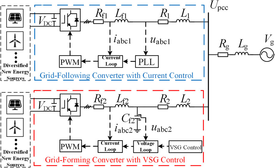
Figure 1. Parallel topology of grid-connected converters with GFL and GFM.

The fundamental concept of the HGS system is to combine grid-following and grid-forming control strategies in parallel, thereby integrating the respective characteristics of these two control approaches. The grid-following converter employs a PLL for synchronization control, and its control structure includes sampling, the PLL, inner current control loops, and a PWM generator. In contrast, the grid-forming converter adopts a more mature Virtual Synchronous Generator (VSG) control strategy. Its control circuit primarily consists of active power and reactive power loops, coordinate transformation, dual-loop voltage and current control, and PWM signal modulation. The two converters are connected to the main power grid via PCC.

In Figure 1, V_DC is a constant DC voltage; R_f1, L_f1, R_f2, and L_f2 are the filter resistances and filter inductances for the GFL and GFM converters, respectively; C_f2 is the filter capacitor for the GFM converter; R₁, L₁, R₂, and L₂ are the line resistances and line inductances for the GFL and GFM converters, respectively; R_g and L_g represent the line resistance and inductance between the PCC and the grid; U_pcc is the voltage at the PCC; i_abc1 and i_abc2 are the converter-side currents for the GFL and GFM converters, respectively; u_abc1 and u_abc2 are the output voltages for the GFL and GFM converters, respectively; V_g is the grid voltage.

2.2 Grid-following converter based on current control

The control system of the GFL is shown in Figure 2. The core of the GFL control strategy is the PLL, and its control structure is shown in Figure 3. The PLL synchronizes the generating unit with the grid by estimating and tracking the phase of the grid voltage u_abc1. The outer-loop power control compares the reference values with the actual values to generate an error signal, which serves as the reference for the inner-loop current control. The inner-loop current control generates modulation signals, which are then processed by the PWM stage.

Figure 2

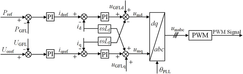
Figure 2. The control system of the GFL.

Figure 3

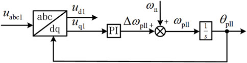
Figure 3. Schematic diagram of phase locked loop.

The mathematical model of the PLL can be expressed as follows:

$\left\{\begin{array}{l}\frac{\mathit{d}{\mathit{\theta }}_{\mathbf{\text{pll}}}}{\mathit{d}\mathit{t}}={\mathit{\omega }}_{\mathbf{\text{pll}}}\\ \frac{\mathit{d}{\mathit{\omega }}_{\mathbf{\text{pll}}}}{\mathit{d}\mathit{t}}={\mathit{k}}_{\mathbf{i}}{\mathit{u}}_{\mathbf{q}\mathbf{1}}+{\mathit{k}}_{\mathbf{p}}\frac{\mathit{d}{\mathit{u}}_{\mathbf{q}\mathbf{1}}}{\mathit{d}\mathit{t}}\end{array}\right.(1)$

In Equation 1: θ_pll is the output phase angle of the PLL; ω_pll is the output angular frequency of the PLL; u_d1 and u_q1 are the d-axis and q-axis voltages of the grid-connected point, respectively; k_i and k_p are the proportional and integral gains of the PI controller. θ_pll is used as the angle for the Park transformation, achieving decoupled control of active and reactive power by aligning u_abc1 with the d-axis, ensuring that u_q1 = 0.

The PLL is used to provide the reference angle for the Park transformation. By aligning u_abc1 to the d-axis, such that u_q1 = 0, decoupled control of active and reactive power is achieved. This ensures precise power regulation and synchronization of the system with the grid.

$\left\{\begin{array}{l}{\mathit{i}}_{\mathbf{\text{dref}}}={\mathit{k}}_{\mathbf{p}\_\mathbf{p}}\left({\mathit{P}}_{\mathbf{\text{ref}}}-{\mathit{P}}_{\mathbf{\text{GFL}}}\right)+{\mathit{k}}_{\mathbf{i}\_\mathbf{p}}\left({\mathit{P}}_{\mathbf{\text{ref}}}-{\mathit{P}}_{\mathbf{\text{GFL}}}\right)/\mathit{s}\\ {\mathit{i}}_{\mathbf{\text{dref}}}={\mathit{k}}_{\mathbf{p}\_\mathbf{u}\mathbf{\text{dc}}}\left({\mathit{U}}_{\mathbf{\text{dcref}}}-{\mathit{U}}_{\mathbf{\text{dc}}}\right)+{\mathit{k}}_{\mathbf{i}\_\mathbf{u}\mathbf{\text{dc}}}\left({\mathit{U}}_{\mathbf{\text{dcref}}}-{\mathit{U}}_{\mathbf{\text{dc}}}\right)/\mathit{s}\end{array}\right.(2)$

$\left\{\begin{array}{l}{\mathit{i}}_{\mathbf{\text{qref}}}={\mathit{k}}_{{\mathbf{p}}_{-}\mathbf{\text{uo}}}\left({\mathit{U}}_{\mathbf{\text{oref}}}-{\mathit{U}}_{\mathbf{\text{GFL}}}\right)+{\mathit{k}}_{{\mathbf{i}}_{-}\mathbf{\text{uo}}}\left({\mathit{U}}_{\mathbf{\text{oref}}}-{\mathit{U}}_{\mathbf{\text{GFL}}}\right)/\mathit{s}\\ {\mathit{i}}_{\mathbf{\text{qref}}}={\mathit{k}}_{{\mathbf{p}}_{-}\mathbf{q}}\left({\mathit{Q}}_{\mathbf{\text{ref}}}-{\mathit{Q}}_{\mathbf{\text{GFL}}}\right)+{\mathit{k}}_{{\mathbf{i}}_{-}\mathbf{q}}\left({\mathit{Q}}_{\mathbf{\text{ref}}}-{\mathit{Q}}_{\mathbf{\text{GFL}}}\right)/\mathit{s}\end{array}\right.(3)$

In Equations 2, 3, i_dref and i_qref represent the d-axis and q-axis reference currents, respectively. k_{p_p} and k_{i_p}, k_{p_udc} and k_{i_udc}, k_{p_uo} and k_{i_uo}, and k_{p_q} and k_{i_q} are the proportional and integral gains of the respective PI controllers. P_ref denotes the active power reference value, and Q_ref represents the reactive power reference value. U_dcref is the reference value for the DC-side voltage, while U_oref is the reference value for the PCC voltage. Finally, U_GFL indicates the output voltage magnitude of the GFL converter.

The mathematical model of the inner current loop can be expressed as follows:

$\left\{\begin{array}{l}{\mathit{u}}_{\mathbf{\text{md}}}={\mathit{u}}_{\mathbf{\text{GFLd}}}+{\mathit{k}}_{\mathbf{p}\_\mathbf{i}}\left({\mathit{i}}_{\mathbf{\text{dref}}}-{\mathit{i}}_{\mathbf{d}}\right)+{\mathit{k}}_{\mathbf{i}\_\mathbf{i}}\left({\mathit{i}}_{\mathbf{\text{dref}}}-{\mathit{i}}_{\mathbf{d}}\right)/\mathit{s}-\mathit{\omega }{\mathit{L}}_{\mathbf{f}}{\mathit{i}}_{\mathbf{q}}\\ {\mathit{u}}_{\mathbf{\text{mq}}}={\mathit{u}}_{\mathbf{\text{GFLq}}}+{\mathit{k}}_{\mathbf{p}\_\mathbf{i}}\left({\mathit{i}}_{\mathbf{\text{qref}}}-{\mathit{i}}_{\mathbf{q}}\right)+{\mathit{k}}_{\mathbf{i}\_\mathbf{i}}\left({\mathit{i}}_{\mathbf{\text{qref}}}-{\mathit{i}}_{\mathbf{q}}\right)/\mathit{s}+\mathit{\omega }{\mathit{L}}_{\mathbf{f}}{\mathit{i}}_{\mathbf{d}}\end{array}\right.(4)$

In Equation 4, u_md and u_mq represent the d-axis and q-axis components of the modulation signal, respectively. k_{p_i} and k_{i_i} are the proportional and integral gains of the PI controller, respectively. L_fi_q and L_fi_d denote the decoupling control terms.

2.3 Grid-forming converter based on VSG control

The control part of a VSG includes an active power loop, a reactive power loop, dual voltage-current control loops, and PWM signal modulation. The core of the control is the active and reactive power loops. VSG achieves synchronization with the grid by mimicking the rotor characteristic equations of a synchronous generator. Consequently, a grid-forming converter based on virtual synchronous generator control possesses the external characteristics of a synchronous generator. The schematic diagram is shown in Figure 4.

Figure 4

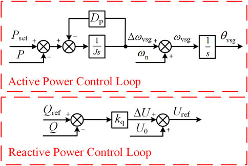
Figure 4. Virtual synchronous machine control schematic diagram.

The control system of GFM converter is shown in Figure 5. The voltage control, current control, and PWM generator of the GFM converter are consistent with those of the grid-following converter.

Figure 5

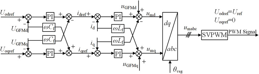
Figure 5. The control system of GFM converter.

The GFM converter achieves control over its output active and reactive power through the active power loop and reactive power loop. The mathematical model of the active power loop under VSG control can be expressed as follows:

$\left\{\begin{array}{l}\frac{\mathit{d}{\mathit{\theta }}_{\mathbf{\text{vsg}}}}{\mathit{d}\mathit{t}}={\mathit{\omega }}_{\mathbf{\text{vsg}}}\\ \mathit{J}\frac{\mathit{d}{\mathit{\omega }}_{\mathbf{\text{vsg}}}}{\mathit{d}\mathit{t}}={\mathit{P}}_{\mathbf{\text{set}}}-\mathit{P}-{\mathit{D}}_{\mathbf{p}}\left({\mathit{\omega }}_{\mathbf{\text{vsg}}}-{\mathit{\omega }}_{\mathbf{n}}\right)\end{array}\right.(5)$

In Equation 5: θ_vsg is the output phase angle of the VSG; ω_vsg is the derivative of θ_vsg; P_set is the input mechanical power; P is the output active power of the VSG; ω_n is the nominal angular frequency; J is the moment of inertia; and D_p is the damping coefficient.

The active power loop adjusts θ_vsg to regulate the output active power P of the VSG, ultimately ensuring that P = P_set.

The mathematical model of the reactive power loop can be expressed as:

${\mathit{U}}_{\mathbf{\text{ref}}}={\mathit{U}}_{\mathbf{0}}+{\mathit{k}}_{\mathbf{q}}\left({\mathit{Q}}_{\mathbf{\text{ref}}}-\mathit{Q}\right)(6)$

In Equation 6: U_ref is the output voltage of the VSG; U₀ is the set value of the output voltage; k_q is the droop coefficient of the reactive power loop; Q_ref is the reactive power reference value; and Q is the output reactive power of the VSG.

The reactive power loop adjusts the output voltage reference value based on the output reactive power.

3 Mathematical modeling of HGS

3.1 The mathematical model and transient characteristics of the grid-connected system

The bandwidth of the current loop in the GFL is significantly larger than the bandwidth of the PLL. By ignoring the dynamic process of the current loop, the GFL can be approximated as a current source. Similarly, in the GFM, the adjustment speed of the inner voltage and current loops is much faster than that of the active and reactive power loops. By neglecting the dynamic process of the inner voltage and current loops, the GFM can be approximated as a voltage source (Li et al., 2021). Circuit impedance is considered negligible, and the phase angle of the grid voltage is taken as the reference angle (Gursoy et al., 2023).The equivalent circuit diagram of Figure 1 is shown in Figure 6.

Figure 6

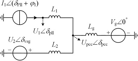
Figure 6. HGS equivalent circuit diagram.

In this figure, I₁ is the RMS value of the output current of the current-controlled converter; U₁ is the RMS value of the output voltage of the GFL; θ_pll is the phase angle difference between the PLL and the grid, corresponding to the power angle of a synchronous generator, and for convenience, it will be referred to as the power angle hereafter; φ₁ is the phase angle difference between voltage U₁ and current I₁; U₂ is the RMS value of the output voltage of the GFM; δ_vsg is the power angle of the GFM; V_g is the RMS value of the grid voltage.

According to the superposition theorem, the PCC voltage U_pcc∠δ_pcc in Figure 6 can be expressed in the stationary reference frame as:

${\mathit{U}}_{\mathbf{\text{pcc}}}\angle {\mathit{\delta }}_{\mathbf{\text{pcc}}}=\mathit{j}{\mathit{k}}_{\mathbf{1}}{\mathit{I}}_{\mathbf{1}}\angle \left({\mathit{\delta }}_{\mathbf{\text{pcc}}}+{\mathit{\phi }}_{\mathbf{1}}\right)+{\mathit{k}}_{\mathbf{2}}{\mathit{U}}_{\mathbf{2}}\angle {\mathit{\delta }}_{\mathbf{\text{vsg}}}+{\mathit{k}}_{\mathbf{3}}{\mathit{V}}_{\mathbf{g}}\angle \mathbf{0}°(7)$

In Equation 7: $k_1={\omega }_{\mathbf{\text{pll}}}\frac{L_2{L}_{\mathrm{g}}}{L_2+L_{\mathrm{g}}};k_2=\frac{L_{\mathrm{g}}}{L_2+L_{\mathrm{g}}};k_3=\frac{L_2}{L_2+L_{\mathrm{g}}}$.

The point where the PLL measures the voltage is U₁∠δ_pll, which can be expressed as:

${\mathit{U}}_{\mathbf{1}}\angle {\mathit{\delta }}_{\mathbf{\text{pll}}}=\mathit{j}{\mathit{k}}_{\mathbf{4}}{\mathit{I}}_{\mathbf{1}}\angle \left({\mathit{\delta }}_{\mathbf{\text{pll}}}+{\mathit{\phi }}_{\mathbf{1}}\right)+{\mathit{k}}_{\mathbf{2}}{\mathit{U}}_{\mathbf{2}}\angle {\mathit{\delta }}_{\mathbf{\text{vsg}}}+{\mathit{k}}_{\mathbf{3}}{\mathit{V}}_{\mathbf{g}}\angle \mathbf{0}°(8)$

In Equation 8: $k_4={\omega }_{\mathbf{\text{pll}}}{L}_1+{\omega }_{\mathbf{\text{pll}}}\frac{L_2{L}_{\mathrm{g}}}{L_2+L_{\mathrm{g}}}$.

Transforming Equation 8 to the dq rotating reference frame based on the PLL, the q-axis voltage of U₁ can be obtained as:

${\mathit{u}}_{\mathbf{q}\mathbf{1}}={\mathit{k}}_{\mathbf{4}}{\mathit{i}}_{\mathbf{d}\mathbf{1}}+{\mathit{k}}_{\mathbf{2}}{\mathit{U}}_{\mathbf{2}}\mathbf{sin}\left({\mathit{\delta }}_{\mathbf{\text{vsg}}}-{\mathit{\delta }}_{\mathbf{\text{pll}}}\right)-{\mathit{k}}_{\mathbf{3}}{\mathit{V}}_{\mathbf{g}}\mathbf{sin}{\mathit{\delta }}_{\mathbf{\text{pll}}}(9)$

In Equation 9: typically, δ_vsg, δ_pll∈[0,π/2].

Comparing Equation 9 with the case of a single GFL connected to the grid, it can be observed that the q-axis voltage u_q1 of the GFL has an additional impedance drop coupling term (Paquette and Divan, 2015). The magnitude of this coupling term is related to k₂, U₂, δ_vsg, and δ_pll, indicating that the power angle of the PLL is also influenced by the GFM power angle δ_vsg.

From Figure 6, the single-phase output complex power of the GFM can be expressed as:

${\dot{\mathit{S}}}_{\mathbf{2}}={\mathit{U}}_{\mathbf{2}}\angle {\mathit{\delta }}_{\mathbf{\text{vsg}}}{\left(\frac{{\mathit{U}}_{\mathbf{2}}\angle {\mathit{\delta }}_{\mathbf{\text{vsg}}}-{\mathit{U}}_{\mathbf{\text{pcc}}}\angle {\mathit{\delta }}_{\mathbf{\text{pcc}}}}{\mathit{j}{\mathit{X}}_{\mathbf{2}}}\right)}^{\ast }(10)$

In Equation 10, X₂ = ω_n L₂, where ω_n is the nominal angular frequency.

Substituting Equation 7 into Equation 10, we obtain:

${\mathit{P}}_{\mathbf{2}}=\frac{{\mathit{k}}_{\mathbf{3}}{\mathit{U}}_{\mathbf{2}}{\mathit{V}}_{\mathbf{g}}}{{\mathit{X}}_{\mathbf{2}}}\mathbf{sin}{\mathit{\delta }}_{\mathbf{\text{vsg}}}-\frac{{\mathit{k}}_{\mathbf{1}}{\mathit{U}}_{\mathbf{2}}{\mathit{I}}_{\mathbf{1}}}{{\mathit{X}}_{\mathbf{2}}}\mathbf{cos}\left({\mathit{\delta }}_{\mathbf{\text{vsg}}}-{\mathit{\delta }}_{\mathbf{\text{pll}}}-{\mathit{\phi }}_{\mathbf{1}}\right)(11)$

${\mathit{Q}}_{\mathbf{2}}=\frac{{\mathit{U}}_{\mathbf{2}}^{\mathbf{2}}-{\mathit{k}}_{\mathbf{2}}{\mathit{U}}_{\mathbf{2}}^{\mathbf{2}}}{{\mathit{X}}_{\mathbf{2}}}-\frac{{\mathit{k}}_{\mathbf{3}}{\mathit{U}}_{\mathbf{2}}{\mathit{V}}_{\mathbf{g}}}{{\mathit{X}}_{\mathbf{2}}}\mathbf{cos}{\mathit{\delta }}_{\mathbf{\text{vsg}}}-\frac{{\mathit{k}}_{\mathbf{1}}{\mathit{U}}_{\mathbf{2}}{\mathit{I}}_{\mathbf{1}}}{{\mathit{X}}_{\mathbf{2}}}\mathbf{sin}\left({\mathit{\delta }}_{\mathbf{\text{vsg}}}-{\mathit{\delta }}_{\mathbf{\text{pll}}}-{\mathit{\phi }}_{\mathbf{1}}\right)(12)$

From Equations 11, 12, it can be seen that the GFL affects both the active power loop and the reactive power loop of the GFM. Compared to the single machine case, an additional active power coupling term and a reactive power coupling term are introduced. The magnitude of this impact is related to k₁、U₂、I₁、X₂、δ_vsg, δ_pll, and φ₁. The power angle of the GFM is also influenced by the output current I₁ of the GFL. By calculating the three-phase active power using Equation 11 and substituting it into Equation 5, it can be obtained that the GFM in steady state satisfies Equation 13.

${\mathit{P}}_{\mathbf{\text{set}}}-\mathbf{3}\frac{{\mathit{k}}_{\mathbf{3}}{\mathit{U}}_{\mathbf{2}}{\mathit{V}}_{\mathbf{g}}}{{\mathit{X}}_{\mathbf{2}}}\mathbf{sin}{\mathit{\delta }}_{\mathbf{\text{vsg}}}+\mathbf{3}\frac{{\mathit{k}}_{\mathbf{1}}{\mathit{U}}_{\mathbf{2}}{\mathit{I}}_{\mathbf{2}}}{{\mathit{X}}_{\mathbf{2}}}\mathbf{cos}\left({\mathit{\delta }}_{\mathbf{\text{vsg}}}-{\mathit{\delta }}_{\mathbf{\text{pll}}}-{\mathit{\phi }}_{\mathbf{1}}\right)=\mathbf{0}(13)$

In summary, the transient analysis model of the HGS can be obtained, as shown in Figure 7. It can be seen that the integration of the GFL adds a power coupling term to the GFM; similarly, the GFM adds an impedance drop coupling term to the GFL (Zhang et al., 2024).

Figure 7

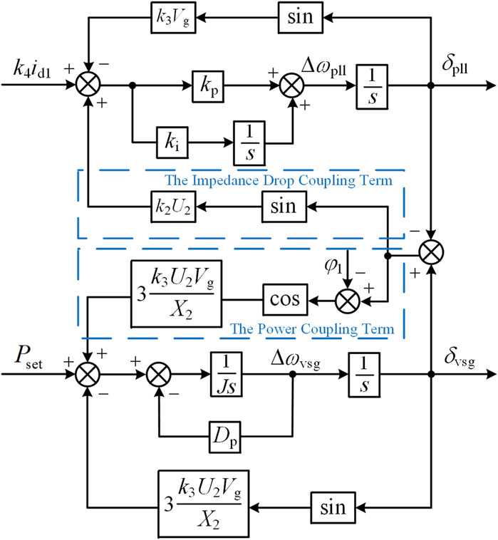
Figure 7. Transient analysis model of HGS.

3.2 Transient stability analysis considering coupling effects

Setting Equation 9 to 0, the condition for the PLL to have an equilibrium point can be obtained as:

$\sqrt{{\left(\frac{{\mathit{k}}_{\mathbf{2}}{\mathit{U}}_{\mathbf{2}}}{{\mathit{k}}_{\mathbf{4}}}\right)}^{\mathbf{2}}+{\left(\frac{{\mathit{k}}_{\mathbf{3}}{\mathit{V}}_{\mathbf{g}}}{{\mathit{k}}_{\mathbf{4}}}\right)}^{\mathbf{2}}+\mathbf{2}\frac{{\mathit{k}}_{\mathbf{2}}{\mathit{k}}_{\mathbf{3}}{\mathit{U}}_{\mathbf{2}}{\mathit{V}}_{\mathbf{g}}}{{\mathit{k}}_{\mathbf{4}}^{\mathbf{2}}}\mathbf{cos}{\mathit{\delta }}_{\mathbf{\text{vsg}}}}\ge {\mathit{i}}_{\mathbf{d}\mathbf{1}}(14)$

When the GFM operates stably, δ_vsg ∈[0, π/2]. If $i_{\mathrm{d}1}>\frac{k_2{U}_2+k_3{V}_{\mathrm{g}}}{k_4}$, then Equation 14 cannot be satisfied, and there is no equilibrium point for the PLL. If $i_{\mathrm{d}1}\le \frac{k_2{U}_2+k_3{V}_{\mathrm{g}}}{k_4}$, then Equation 14 can be satisfied, and an equilibrium point exists for the PLL.

From Equation 13, it can be seen that the presence of I₁ increases δ_vsg, reducing the stability margin of the GFM. The magnitude of δ_vsg is directly proportional to k₁, U₂, and I₁, and inversely proportional to X₂. If I₁ is too large, it may cause the initially stable GFM to lose power angle stability. If the GFM loses power angle stability due to a fault or other reasons, its output angle δ_vsg increases indefinitely. As indicated by Equation 14, when δ_vsg = 2kπ + π, k∈Z, the impact on the PLL is maximized, leading to two possible situations: ① If Equation 14 is not satisfied, the GFL becomes unstable. ② If Equation 14 is satisfied, since δ_vsg increases indefinitely, Equation 9 remains in a state of adjustment and cannot stabilize or converge to 0, indicating that the GFL becomes unstable.

Therefore, transient instability in the GFM will trigger a chain reaction, causing transient instability in the GFL.

From Equation 13, the GFM has a steady-state point when the following condition is satisfied:

$\sqrt{\mathbf{9}{\left(\frac{{\mathit{k}}_{\mathbf{3}}{\mathit{U}}_{\mathbf{2}}{\mathit{V}}_{\mathbf{g}}}{{\mathit{X}}_{\mathbf{2}}}\right)}^{\mathbf{2}}+\mathbf{9}{\left(\frac{{\mathit{k}}_{\mathbf{1}}{\mathit{U}}_{\mathbf{2}}{\mathit{I}}_{\mathbf{1}}}{{\mathit{X}}_{\mathbf{2}}}\right)}^{\mathbf{2}}-\mathbf{18}\frac{{\mathit{k}}_{\mathbf{1}}{\mathit{k}}_{\mathbf{3}}{\mathit{U}}_{\mathbf{2}}^{\mathbf{2}}{\mathit{V}}_{\mathbf{g}}{\mathit{I}}_{\mathbf{1}}}{{\mathit{X}}_{\mathbf{2}}^{\mathbf{2}}}\mathbf{sin}\left({\mathit{\delta }}_{\mathbf{\text{pll}}}+{\mathit{\phi }}_{\mathbf{1}}\right)}\ge {\mathit{P}}_{\mathbf{\text{set}}}(15)$

When the GFL operates stably, δ_pll ∈ [0, π/2] and φ₁ ∈ [-π/2, 0]. If ${\mathrm{P}}_{\mathbf{\text{set}}}>3\frac{{\mathrm{k}}_3{\mathrm{U}}_2{\mathrm{V}}_{\mathrm{g}}+{\mathrm{k}}_1{\mathrm{U}}_2{\mathrm{I}}_1}{{\mathrm{X}}_2}$, Equation 15 cannot be satisfied, and there is no equilibrium point for the GFM. If ${\mathrm{P}}_{\mathbf{\text{set}}}\le 3\frac{{\mathrm{k}}_3{\mathrm{U}}_2{\mathrm{V}}_{\mathrm{g}}+{\mathrm{k}}_1{\mathrm{U}}_2{\mathrm{I}}_1}{{\mathrm{X}}_2}$ , then Equation 15 can be satisfied, and an equilibrium point exists for the GFM.

From Equation 9, it can be seen that when δ_vsg > δ _pll, δ _pll increases, and the stability margin of the GFL decreases. When δ_vsg < δ_pll, δ_pll decreases, and the stability margin of the GFL increases. When δ_vsg = δ_pll, the coupling term is zero, and δ_pll is not affected by the GFM. If the GFL loses synchronization stability due to a fault or other reasons, the PLL will have no equilibrium point, causing the power angle δ_pll to increase indefinitely, thereby affecting the GFM. There are two possible scenarios: ① If Equation 15 is not satisfied, the GFM becomes unstable. ② If Equation 15 is satisfied, due to δ_pll increasing indefinitely, Equation 13 remains in a state of adjustment and cannot converge to zero, indicating that the GFM becomes unstable.

Therefore, when the GFL experiences transient instability, the increase in its output phase also causes the GFM to experience transient instability.

In summary, it is essential to ensure the simultaneous stability of both converters; instability in either one will affect the stability of the other.

Additionally, during grid voltage sag, the GFM, being a voltage source type, can experience transient overcurrent and steady-state overcurrent. Under fault conditions, the circuit satisfies:

$\left({\mathit{L}}_{\mathbf{2}}+{\mathit{L}}_{\mathbf{g}}\right)\frac{\mathit{d}{\mathit{i}}_{\mathbf{2}\mathbf{F}}}{\mathit{d}\mathit{t}}={\mathit{u}}_{\mathbf{2}\mathbf{F}}-{\mathit{\nu }}_{\mathbf{\text{gF}}}-{\mathit{L}}_{\mathbf{g}}\frac{\mathit{d}{\mathit{i}}_{\mathbf{1}}}{\mathit{d}\mathit{t}}(16)$

In Equation 16: i_2F is the instantaneous value of the GFM output current during a fault; u_2F is the instantaneous value of the GFM output voltage during a fault; v_gF is the instantaneous value of the grid voltage during a fault; i₁ is the instantaneous value of the output current of the current-controlled converter.

From Equation 16, it can be seen that the presence of the GFL can reduce the fault current of the GFM.

During a fault, reducing the GFL output current i_d1 not only ensures the existence of the PLL equilibrium point, but also, as seen from Equation 9, the reduction of i_d1 can slow down the acceleration process of the GFL output ω_pll during the fault, thereby reducing the deviation of ω_pll. Since the inertia of the GFM is much larger than the equivalent inertia of the GFL, the increase rate of δ_vsg is slower than that of δ_pll during a fault. Additionally, because the fault duration is short, during the fault, (δ_vsg − δ_pll) ∈ [-π/2, 0] (Cheng et al., 2022). For purely active power output, φ₁ = 0, and the reduction in i_d1 is much greater than the change in the cosine function, so the effect of the cosine function can be ignored. Therefore, when i_d1 is reduced, the power coupling term in Equation 11 is also reduced. From Equation 5, it can be seen that this also helps to slow down the acceleration of the GFM output ω_vsg during the fault, reducing the deviation of ω_vsg. The phase plane diagram of the HGS under different i_d1 conditions during a fault is shown in Figure 8.

Figure 8

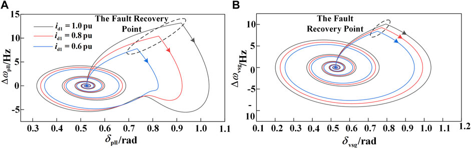
Figure 8. Phase portrait of different i_d1 of GFL. (A) The phase plane of the GFL under fault conditions. (B) The phase plane of the GFM under fault conditions.

From Figure 8, it can be observed that reducing the active current of the GFL can slow down the acceleration process of both the GFL and GFM during a fault, thereby improving the synchronization stability of the two converters. Moreover, the smaller the i_d1, the better the synchronization stability of the two converters; conversely, the larger the i_d1, the worse the synchronization stability of the two converters.

During a fault, reducing the input mechanical power P_set of the GFM not only ensures the existence of the GFM’s equilibrium point but, as shown in Equation 5, also slows down the acceleration process of the GFM’s output ω_vsg during the fault, reducing the deviation of ω_vsg. A decrease in P_set during a fault causes the δ_vsg of the GFM, which has inertia, to increase more slowly than δ_pll. The smaller the P_set, the slower the increase of δ_vsg, the larger the | δ_vsg − δ_pll |, and the smaller the impedance drop coupling term in Equation 9, resulting in a smaller deviation of the GFL’s output ω_pll. The phase plane diagram of the HGS under different P_set conditions during a fault is shown in Figure 9.

Figure 9

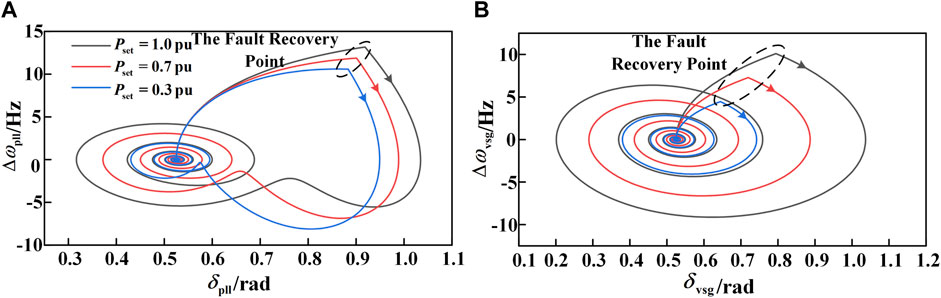
Figure 9. Phase portrait of different P_set of GFM. (A) The phase plane of the GFL under fault conditions. (B) The phase plane of the GFM under fault conditions.

From Figure 9, it can also be seen that reducing the input mechanical power P_set of the GFM can similarly slow down the acceleration process of both the GFM and GFL during a fault, thereby enhancing the synchronization stability of the two converters. Moreover, the smaller the P_set, the better the synchronization stability of the two converters; conversely, the larger the P_set, the worse the synchronization stability of the two converters.

4 Fault ride-through control of the HGS

During a low voltage sag fault in the grid, the HGS faces three issues: power angle instability caused by the power imbalance between the GFM and GFL; outputting reactive current in compliance with grid codes to support the grid; and the risk of overcurrent due to the large short-circuit current of the GFM, which threatens power electronic equipment.

From the previous analysis, it is known that reducing i_d1 and P_set during a grid fault helps ensure the existence of the equilibrium points of the GFL and GFM, and simultaneously enhances the transient stability of both converters. However, the conditions for the existence of the equilibrium points of both converters are coupled through the GFL power angle δ_pll, the GFL output current I₁, the GFM power angle δ_vsg, and the GFM output voltage U₂. Directly controlling the power angles by adjusting i_d1 and P_set is quite challenging. Therefore, this paper first determines the values of the GFM power angle δ_vsgF, the fault currents I_1F and I_2F during the fault, and then calculates the required VSG output voltage U_2F and mechanical power P_setF based on the power angles.

4.1 Equations transient power angle control

During a grid fault, while maintaining power angle stability, the GFM power angle δ_vsgF is adjusted based on the extent of the grid voltage sag to modify the reactive component of the output current during the fault, thereby supporting the grid. The adjustment rules are as follows:

$\begin{array}{rr}{\mathit{\delta }}_{\mathbf{\text{vsgF}}}& =\left\{\begin{array}{ll}\frac{{\mathit{V}}_{\mathbf{\text{gF}}}}{{\mathit{V}}_{\mathbf{g}}}{\mathit{\delta }}_{\mathbf{2}}^{\mathbf{0}}& ,\mathbf{0.2}<\frac{{\mathit{V}}_{\mathbf{\text{gF}}}}{{\mathit{V}}_{\mathbf{g}}}<\mathbf{0.9}\\ \mathbf{0}& ,\frac{{\mathit{V}}_{\mathbf{\text{gF}}}}{{\mathit{V}}_{\mathbf{g}}}\le \mathbf{0.2}\end{array}\right.\end{array}(17)$

In Equation 17, δ 0 2 is the power angle of the GFM before the fault;V_gF is the RMS value of the grid phase voltage after the fault. During the fault, by adjusting P_set, we can control the power angle of the GFM, making it reach δ_vsgF under the corresponding V_gF.

According to Equation 14, the equilibrium point of the PLL is not only related to the output current i_d1 but also affected by the inductances L₁, L₂, and L_g. Therefore, by adjusting only the current, especially in a weak grid environment, it is impossible to ensure the existence of the equilibrium point. Hence, the output phase angle θ_vsg of the GFM is transmitted to the PLL. However, under this circumstance, the PLL becomes an open-loop system with a steady-state error, making it impossible to precisely align Ů₁ with the d-axis.

From Figure 10A, it can be seen that there is a fixed angular difference φ between Ů₁ and the d-axis d_GFL of the GFL. Therefore, the angle of the GFL needs to be adjusted by adding a fixed angle φ on the basis of θ_vsg. This can be obtained by measuring the deviation of u_q1 and applying PI control.

$\left\{\begin{array}{c}{\mathit{\theta }}_{\mathbf{\text{pll}}}={\mathit{\theta }}_{\mathbf{\text{vsg}}}+\mathit{\varphi }\\ \mathit{\varphi }={\mathit{k}}_{\mathbf{p}}{\mathit{u}}_{\mathbf{q}\mathbf{1}}+{\mathit{k}}_{\mathbf{i}}\int {\mathit{u}}_{\mathbf{q}\mathbf{1}}\end{array}\right.(18)$

Figure 10

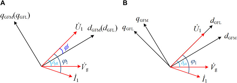
Figure 10. Voltage vector diagram. (A) Based on the GFM rotating coordinate system. (B) Based on the GFL rotating coordinate system.

Using Equation 18, an improved PLL based on the grid-forming model can be obtained, which can also precisely align U₁ with the d-axis of the two-phase rotating coordinate system of the GFL, as shown in Figure 10B. At this point, the active power and reactive power of the GFL are decoupled.

The P_setF during the fault can be obtained as:

${\mathit{P}}_{\mathbf{\text{setF}}}=\mathbf{3}\frac{{\mathit{k}}_{\mathbf{3}}{\mathit{U}}_{\mathbf{2}}{\mathit{V}}_{\mathbf{\text{gF}}}}{{\mathit{X}}_{\mathbf{2}}}\mathbf{sin}{\mathit{\delta }}_{\mathbf{\text{vsgF}}}-\mathbf{3}\frac{{\mathit{k}}_{\mathbf{1}}{\mathit{U}}_{\mathbf{2}}{\mathit{I}}_{\mathbf{1}}}{{\mathit{X}}_{\mathbf{2}}}\mathbf{cos}\left(\mathit{\varphi }+{\mathit{\phi }}_{\mathbf{1}}\right)(19)$

After introducing the input mechanical power adjustment loop in the GFM and adopting the improved PLL based on the grid-forming model in the GFL, the control block diagrams of the GFM and GFL are shown in Figure 11. In this case, as long as the GFM remains stable, the stability of the GFL can be ensured.

Figure 11

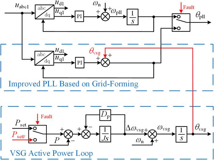
Figure 11. HGS transient power angle control.

4.2 Fault current control

4.2.1 Steady-state current control

Although the GFM is stabilized by adjusting the input mechanical power, this does not effectively suppress the overcurrent phenomenon. Even though the presence of the GFL can reduce the fault current of the GFM, the GFM may still generate a significant fault current when there is a substantial drop in grid voltage. Therefore, when the fault current I_2F exceeds 1.5 times the rated current, the control of the GFM fault current I_2F is as follows:

${\mathit{I}}_{\mathbf{2}\mathbf{F}}=\mathbf{1.5}{\mathit{I}}_{\mathbf{2}\mathbf{n}}(20)$

In Equation 20: I_2n is the rated value of the GFM output current.

Since the GFL is a current source type, it will not generate steady-state overcurrent during a fault. However, to support the grid, it needs to output reactive current. The adjustment rules for the output current of the grid-following type are as follows:

$\begin{array}{ll}{\mathit{I}}_{\mathbf{q}\mathbf{1}\mathbf{F}}& =\left\{\begin{array}{ll}\mathbf{0}& ,\frac{{\mathit{V}}_{\mathbf{\text{gF}}}}{{\mathit{V}}_{\mathbf{g}}}\ge \mathbf{0.9}\\ -\mathbf{1.5}\left(\mathbf{0.9}-\frac{{\mathit{V}}_{\mathbf{\text{gF}}}}{{\mathit{V}}_{\mathbf{g}}}\right){\mathit{I}}_{\mathbf{1}\mathbf{n}}& ,\mathbf{0.2}\le \frac{{\mathit{V}}_{\mathbf{\text{gF}}}}{{\mathit{V}}_{\mathbf{g}}}<\mathbf{0.9}\\ -\mathbf{1.05}{\mathit{I}}_{\mathbf{1}\mathbf{n}}& ,\frac{{\mathit{V}}_{\mathbf{\text{gF}}}}{{\mathit{V}}_{\mathbf{g}}}<\mathbf{0.2}\end{array}\right.\end{array}(21)$

${\mathit{I}}_{\mathbf{d}\mathbf{1}\mathbf{F}}=\left\{\begin{array}{l}\sqrt{{\mathit{I}}_{\mathbf{1}\mathbf{n}}^{\mathbf{2}}-{\mathit{I}}_{\mathbf{q}\mathbf{1}\mathbf{F}}^{\mathbf{2}}},\frac{{\mathit{V}}_{\mathbf{\text{gF}}}}{{\mathit{V}}_{\mathbf{g}}}\ge \mathbf{0.2}\\ \mathbf{0},\frac{{\mathit{V}}_{\mathbf{\text{gF}}}}{{\mathit{V}}_{\mathbf{g}}}<\mathbf{0.2}\end{array}\right.(22)$

In Equations 21, 22: I_1n is the rated value of the GFL output current;I_d1F is the d-axis output current of the GFL during a fault;I_q1F is the q-axis output current of the GFL during a fault.

Based on Equations 17, 21, 22, the values of δ_vsgF, I_q1F, and I_d1F are obtained, respectively. From Equations 7, 9, 11, 20, the following system of equations can be derived:

$\left\{\begin{array}{rr}{\left(\mathit{A}-{\mathit{k}}_{\mathbf{3}}{\mathit{V}}_{\mathbf{g}}\right)}^{\mathbf{2}}+{\mathit{B}}^{\mathbf{2}}-\mathbf{2}{\left(\mathbf{1.5}{\mathit{X}}_{\mathbf{2}}{\mathit{I}}_{\mathbf{2}\mathbf{n}}\right)}^{\mathbf{2}}& =\mathbf{0}\\ {\mathit{k}}_{\mathbf{4}}{\mathit{i}}_{\mathbf{d}\mathbf{1}\mathbf{F}}-{\mathit{k}}_{\mathbf{2}}{\mathit{U}}_{\mathbf{2}\mathbf{F}}\mathbf{sin}\mathit{\varphi }-{\mathit{k}}_{\mathbf{3}}{\mathit{V}}_{\mathbf{g}}\mathbf{sin}\left({\mathit{\delta }}_{\mathbf{\text{vsgF}}}+\mathit{\varphi }\right)& =\mathbf{0}\\ {\mathit{P}}_{\mathbf{\text{sefF}}}=\mathit{C}\mathbf{sin}{\mathit{\delta }}_{\mathbf{\text{vsgF}}}-\mathit{D}\mathbf{cos}\left(\mathit{\varphi }+{\mathit{\phi }}_{\mathbf{\text{lF}}}\right)& \end{array}\right.(23)$

In Equation 23: ${\phi }_{1\mathrm{F}}=\arctan \left(\frac{I_{\mathrm{q}1\mathrm{F}}}{I_{\mathrm{d}1\mathrm{F}}}\right);I_{1\mathrm{F}}=\sqrt{I_{\mathrm{d}1\mathrm{F}}^2+I_{\mathrm{q}1\mathrm{F}}^2};A=U_{2\mathrm{F}}\cos {\delta }_{\mathbf{\text{vsgF}}}+k_1{I}_{1\mathrm{F}}\sin \left({\delta }_{\mathbf{\text{vsgF}}}+\varphi +{\phi }_{1\mathrm{F}}\right)-k_2{U}_{2\mathrm{F}}\cos {\delta }_{\mathbf{\text{vsgF}}};$ $B=U_{2\mathrm{F}}\sin {\delta }_{\mathbf{\text{vsgF}}}-k_1{I}_{1\mathrm{F}}\cos \left({\delta }_{\mathbf{\text{vsgF}}}+\varphi +{\phi }_{1\mathrm{F}}\right)-k_2{U}_{2\mathrm{F}}\sin {\delta }_{\mathbf{\text{vsgF}}};C=3\frac{k_3{U}_{2\mathrm{F}}{V}_{\mathrm{g}}}{X_2}.$

Equation 21 can be solved using numerical methods to obtain the output voltage U_2F of the GFM and the input mechanical power P_setF during a fault. Since the reactive power loop adjusts the output voltage command, this may lead to inaccurate fault current control. Therefore, during a fault, the reactive power loop is locked, and the calculated U_2F is used to replace the output of the reactive power loop.

4.2.2 Steady-state current control

The transient current of the GFL is small and has a minimal impact on the system, so it can be neglected. However, the transient current of the GFM is relatively large, and adjusting the reference voltage of the reactive power loop alone is not effective. If left unchecked, it can damage transistors.

Therefore, transient virtual impedance is used to suppress transient overcurrent. The threshold current Ith for the virtual impedance is set slightly above 1.5 times I_2n. When the detected fault current exceeds Ith, the virtual impedance is activated; otherwise, the virtual impedance remains inactive. By combining the virtual impedance with the adjustment of the reactive power loop, the output voltage of the GFM can be expressed as:

${\mathit{U}}_{\mathbf{\text{ref}}}={\mathit{U}}_{\mathbf{2}\mathbf{F}}-{\mathit{I}}_{\mathbf{2}\mathbf{F}}{\mathit{Z}}_{\mathbf{v}}(24)$

In Equation 24: Z_v is the virtual impedance.

The overall current control block diagram is shown in Figure 12:

Figure 12

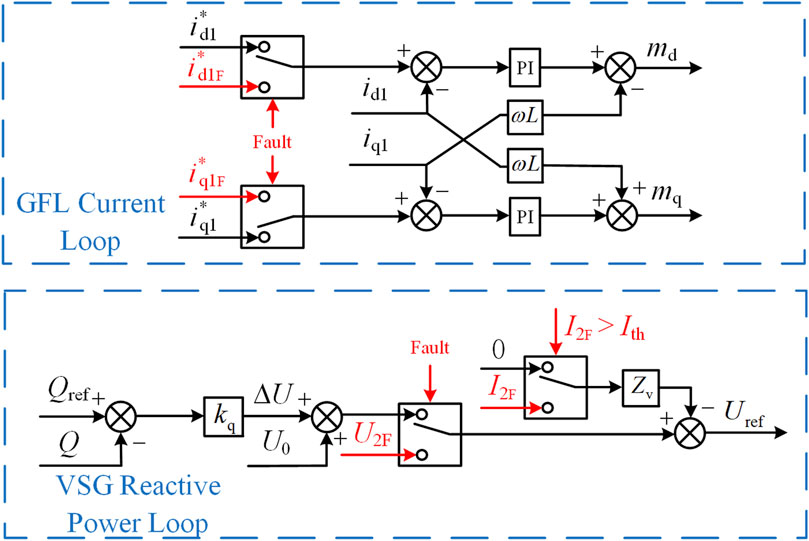
Figure 12. HGS fault current control.

4.3 Fault ride-through control process for HGS

The fault ride-through control process is illustrated in Figure 13. The system operates under normal conditions, monitoring V_g to determine whether a fault has occurred. In the event of a ground fault, the value of V_g decreases.

Figure 13

Figure 13. Fault ride-through control flowchart.

When the grid voltage drops above a specified threshold, the transient current is evaluated to determine whether it exceeds the current-limiting threshold, thereby deciding whether to activate transient virtual impedance control. If the grid voltage falls below the threshold, transient power angle control is first applied to the hybrid system. Using Equations 17, 21, 22, the fault power angle of the GFM converter and the reference current for the GFL converter are determined. Subsequently, the value of P_setF is calculated according to Equation 19.

Next, the fault current of the GFM converter is monitored. If the current exceeds the transient current-limiting threshold, both the reactive power loop and transient virtual impedance control for the GFM converter are activated. If the current only exceeds the steady-state current-limiting threshold of the GFM converter, only the reactive power loop control is applied.

Once the reactive power loop control is engaged in the GFM converter, the previously determined GFM fault power angle and GFL reference current are used to calculate P_setF and U_2F according to Equation 23. When V_g recovers above the threshold value, the hybrid system transitions back to the normal control strategy.

5 Case study

To verify the theoretical analysis and the proposed fault ride-through control strategy, a hybrid grid-connected model of grid-following and GFM, as shown in Figure 1, was built in Matlab/Simulink. The system parameters are listed in Table 1.

Table 1

Table 1. Parameters of HGS.

5.1 Output characteristics of GFM and GFL during fault conditions

When the three-phase grid voltage drops to 0.5, the output currents and power angles of the GFM and GFL are shown in Figure 14. The simulation duration is set to 3 s, with a fault occurring at 0.5 s and clearing at 2 s. As seen in Figure 14, during the fault, the power angles of both the GFM and GFL increase indefinitely. The output currents of the two converters are affected by the power angles, resulting in oscillations. Since the GFM is a voltage source type, its maximum current amplitude reaches three times its rated operating value. The output active and reactive power of both converters also experience oscillations.

Figure 14

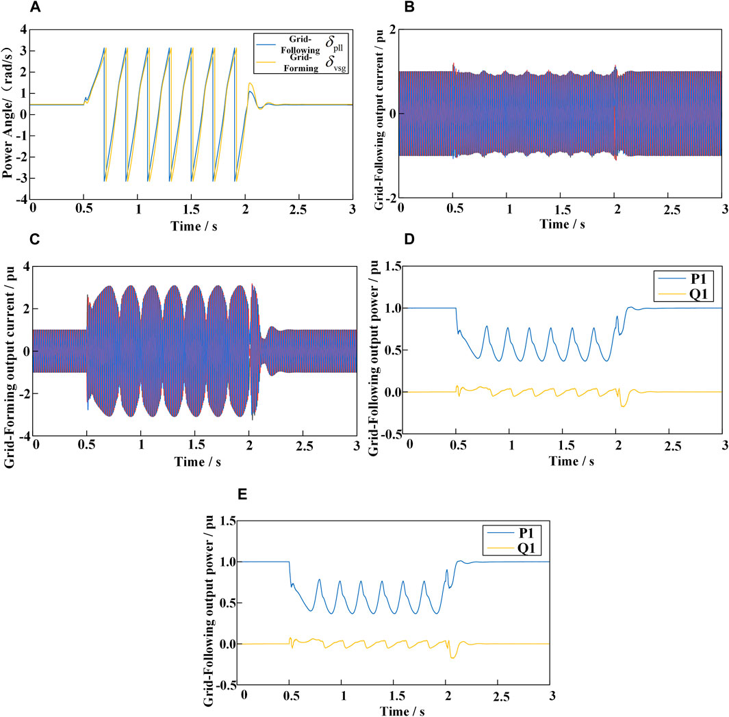
Figure 14. Output waveform under symmetrical fault of grid. (A) Power angle curve. (B) Grid-Following output current. (C) Grid-Forming output current. (D) Grid-Following output power. (E) Grid-Forming output power.

Figure 15A shows the power angle curves of both converters when the d-axis current reference value I *d1 of the grid-following converter is changed from 1 pu to 2.5 pu at 0.5 s and restored to 1 pu at 2 s. Figure 15B shows the power angle curves of both converters when the input mechanical power P_set of the grid-forming converter is changed from 1 pu to 3 pu at 0.5 s and restored to 1 pu at 2 s. Based on the output power angles, it can be seen that the occurrence of power angle instability in the GFL immediately causes power angle instability in the GFM. Similarly, the occurrence of power angle instability in the GFM immediately causes power angle instability in the GFL. This verifies the analysis of the mutual influence between the two converters mentioned earlier.

Figure 15

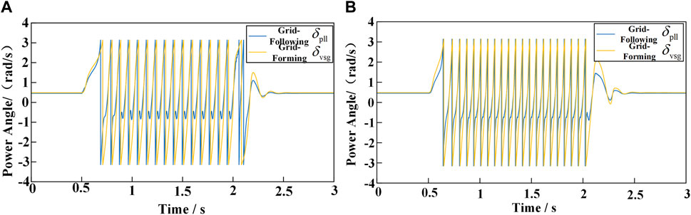
Figure 15. Change the reference value of the inverter. (A) Changing Grid-Following reference current. (B) Changing Grid-Forming input mechanical power.

5.2 Verification of the proposed fault ride-through control strategy

Figure 16 shows the output waveforms when the grid voltage symmetrically drops to 0.4 pu at 0.5 s and rises back to 1 pu at 2 s. During the fault, transient power angle control is applied to the HGS, and both the GFL and GFM remain stable after a brief transient process. As seen in Figure 16B, during the fault, by adjusting the input mechanical power P_set of the GFM and using the improved PLL based on the grid-forming model for the GFL, the power angles of both converters can be kept stable. However, as shown in Figure 16D, the transient current output by the GFM is too large, and the steady-state current also exceeds 1.5 pu, approaching 2 pu. From Figure 16F, it can be seen that this is due to the excessive reactive current output by the GFM. Although reactive current can support the grid, there is still a risk of damaging transistors. Therefore, it is necessary to suppress transient and steady-state overcurrents through fault current control.

Figure 16

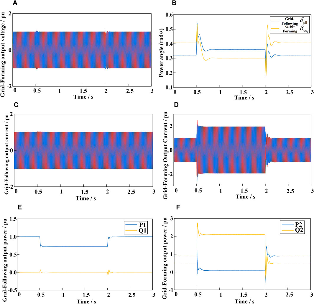
Figure 16. Output waveform under transient power Angle fault ride-through control only. (A) Grid-Forming output voltage. (B) Power angle curve. (C) Grid-Following output current. (D) Grid-Forming output current. (E) Grid-Following output power. (F) Grid-Forming output power.

Figure 17 shows the waveforms of the HGS when transient power angle and fault current control are implemented as the grid voltage symmetrically drops to 0.4 pu. Similarly, the GFL and GFM remain stable after a brief transient process. As shown in Figure 17D, during the fault, by reducing the output voltage of the GFM, the GFM’s output current is precisely controlled to 1.5 pu. Thanks to the virtual impedance, the transient current is also effectively suppressed. As depicted in Figure 17E, the GFL, while remaining stable, is able to provide reactive current in accordance with grid codes, supporting the grid. After the fault is cleared, both converters can return to their pre-fault operating state after a brief transient process.

Figure 17

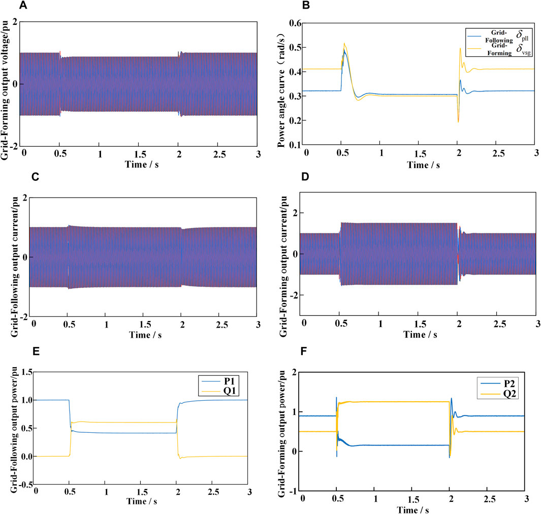
Figure 17. Output waveform under transient power Angle and current fault ride-through control. (A) Grid-Forming output voltage. (B) Power angle curve. (C) Grid-Following output current (D) Grid-Forming output current.(E) Grid-Following output power. (F) Grid-Forming output power.

Figure 18 presents the waveforms of transient power angle and fault current control for the HGS system during a symmetrical grid voltage dip to 0.6 pu. Similarly, both the GFL and GFM converters remain stable after a brief transient process. As shown in Figure 17C, during the fault, the output current of the GFM converter is below 1.5 pu, in contrast to the scenario where the grid voltage symmetrically drops to 0.4 pu. This reduction is attributed to the implementation of virtual impedance, which effectively suppresses transient currents. As depicted in Figure 17D, the GFL converter, while maintaining stability, provides reactive current in compliance with grid codes, thereby supporting the grid. After the fault is cleared, both converters recover to their normal operating conditions following a brief transient period.

Figure 18

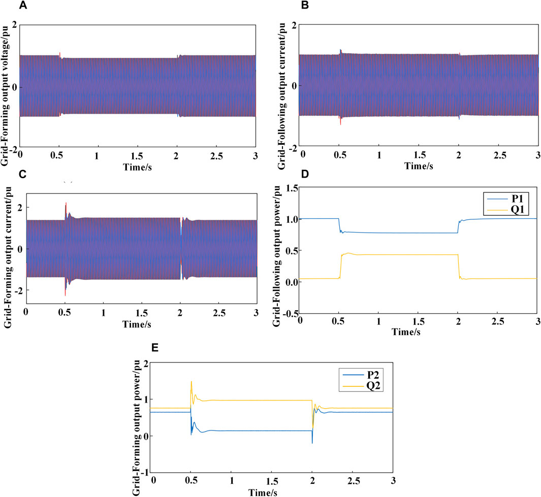
Figure 18. Transient power angle and fault current waveforms under fault ride-through control. (A) Grid-Forming output voltage. (B) Grid-Following output current. (C) Grid-Forming output current. (D) Grid-Following output power. (E) Grid-Forming output power.

6 Conclusion

This paper analyzes the transient stability of HGS with parallel GFL and GFM, and proposes a fault ride-through control strategy considering the interactive effects between GFL and GFM. By establishing a mathematical model of the HGS, the dynamic coupling mechanism between GFM and GFL is revealed, and the fault ride-through problem under symmetrical voltage drops is studied. The main conclusions are as follows:

1) Through the transient stability analysis of the HGS with parallel GFL and GFM, demonstrating that the two are mutually coupled through the grid impedance. The instability of one converter will lead to the instability of the other converter. During a fault, reducing the i_d1 of GFL or the P_set of GFM can simultaneously improve the transient stability of both converters.

2) During a fault, the GFM adjusts the power angle according to the extent of the grid voltage drop and modifies the output voltage while considering the impact of the current injected by the GFL when limiting current. This approach can effectively suppress short-circuit overcurrent and maintain power angle stability. The GFL uses an improved PLL based on grid-forming control, which can effectively prevent GFL instability and inject current into the grid in accordance with grid codes.

3) Considering the interactive effects of GFL and GFM, a fault ride-through control strategy applicable to the HGS is proposed. By setting a threshold current Ith slightly greater than 1.5 I_2n in the GFM, virtual impedance is introduced when the detected fault current exceeds Ith, effectively suppressing transient overcurrent.

4) The transient current of the GFM is relatively large. By setting a threshold current Ith slightly greater than 1.5I_2n in the GFM, virtual impedance is introduced when the detected fault current exceeds Ith, effectively suppressing transient overcurrent. This approach addresses the shortcomings of reactive voltage reference adjustment alone, which is less effective and risks damaging transistors.

This study preliminarily explores the interaction mechanisms and fault ride-through control for GFL and GFM converters under symmetrical faults. However, the transient processes and fault control strategies under asymmetrical faults are more complex. Future work will focus on control strategies for asymmetrical fault conditions.

Data availability statement

The original contributions presented in the study are included in the article/supplementary material, further inquiries can be directed to the corresponding author.

Author contributions

BZ: Conceptualization, Methodology, Writing–original draft. SL: Conceptualization, Validation, Writing–review and editing. ZX: Software, Validation, Writing–review and editing. FD: Data curation, Writing–review and editing. JC: Funding acquisition, Project administration, Resources, Supervision, Writing–review and editing. HW: Formal Analysis, Investigation, Validation, Visualization, Writing–review and editing.

Funding

The author(s) declare that financial support was received for the research, authorship, and/or publication of this article. This research was funded by the Science and Technology Department of Xinjiang under grant No. 2022A01004.

Conflict of interest

Authors BZ, SL, ZX and HW were employed by the company Electric Power Research Institute of State Grid Xinjiang Electric Power Co., Ltd.

The remaining authors declare that the research was conducted in the absence of any commercial or financial relationships that could be construed as a potential conflict of interest.

Generative AI statement

The author(s) declare that no Generative AI was used in the creation of this manuscript.

Publisher’s note

All claims expressed in this article are solely those of the authors and do not necessarily represent those of their affiliated organizations, or those of the publisher, the editors and the reviewers. Any product that may be evaluated in this article, or claim that may be made by its manufacturer, is not guaranteed or endorsed by the publisher.

References

Chen, J., Prystupczuk, F., and O' Donnell, T. (2020). Use of voltage limits for current limitations in grid-forming converters. CSEE J. Power Energy Syst. 6 (2), 259–269. doi:10.17775/CSEEJPES.2019.02660

CrossRef Full Text | Google Scholar

Cheng, H., Shuai, Z., Peng, Y., Huang, W., and Shen, Z. J. (2022). “Coupled problem of transient voltage/angle stability in paralleled synchronous and virtual synchronous generators with dynamic loads,” in 2022 IEEE 5th International Electrical and Energy Conference (CIEEC), Nangjing, China, 2303–2308. doi:10.1109/CIEEC54735.2022.9846152

CrossRef Full Text | Google Scholar

Gao, X., Zhou, D., Anvari-Moghaddam, A., and Blaabjerg, F. (2023). “Analysis of X/R ratio effect on stability of grid-following and grid-forming converters,” in 2023 IEEE 17th International Conference on Compatibility, Power Electronics and Power Engineering (CPE-POWERENG), Tallinn, Estonia, 14-16 June 2023 (IEEE), 1–6.

CrossRef Full Text | Google Scholar

Gu, Y., and Green, T. C. (2023). Power system stability with a high penetration of inverter-based resources. Proc. IEEE 111 (7), 832–853. doi:10.1109/jproc.2022.3179826

CrossRef Full Text | Google Scholar

Gursoy, M., Sadeque, F., Fateh, F., and Mirafzal, B. (2023). “Direct control methods for grid-forming and grid-following inverters,” in 2023 IEEE Energy Conversion Congress and Exposition (ECCE), Nashville, TN, USA, 1081–1088. doi:10.1109/ECCE53617.2023.10361995

CrossRef Full Text | Google Scholar

He, X., Geng, H., Xi, J., and Guerrero, J. M. (2021). Resynchronization analysis and improvement of grid-connected VSCs during grid faults. IEEE J. Emerg. Sel. Top. Power Electron. 9 (1), 438–450. doi:10.1109/jestpe.2019.2954555

CrossRef Full Text | Google Scholar

Huang, Z., Chen, D., Qiu, Y., and Ying, K. (2024). “Optimization of resource allocation for distributed energy consumption based on a meta-heuristic algorithm,” in 2024 3rd International Conference on Energy and Electrical Power Systems (ICEEPS), Guangzhou, China, 198–201. doi:10.1109/ICEEPS62542.2024.10693062

CrossRef Full Text | Google Scholar

IEEE (2022). “Ieee standard for interconnection and interoperability of inverter-based resources (ibrs) interconnecting with associated transmission electric power systems,” in Ieee std 2800-2022 (IEEE), 1–180. doi:10.1109/IEEESTD.2022.9762253

CrossRef Full Text | Google Scholar

Kim, K.-H., Cui, S., and Jung, J.-J. (2024). Current-oriented phase-locked loop method for robust control of grid-connected converter in extremely weak grid. IEEE Trans. Power Electron. 39 (10), 11963–11968. doi:10.1109/tpel.2024.3419445

CrossRef Full Text | Google Scholar

Li, M., Quan, X., Wu, Z., Li, W., Zhu, L., and Hu, Q. (2021). “Modeling and transient stability analysis of mixed-GFM-GFL-based power system,” in 2021 IEEE Sustainable Power and Energy Conference (iSPEC), Nanjing, China, 2755–2759. doi:10.1109/iSPEC53008.2021.9735564

CrossRef Full Text | Google Scholar

Li, Y., Gu, Y., and Green, T. C. (2022). Revisiting grid-forming and grid-following inverters: a duality theory. IEEE Trans. Power Syst. 37 (6), 4541–4554. doi:10.1109/tpwrs.2022.3151851

CrossRef Full Text | Google Scholar

Lu, Y., Cao, W., Zhang, Z., and Hu, B. (2023). “Fault-current limiting strategy for grid-forming converters with virtual impedance from both inner CCL and outer VCL,” in 2023 IEEE 7th Conference on Energy Internet and Energy System Integration (EI2), Hangzhou, China, 1907–1911. doi:10.1109/EI259745.2023.10512712

CrossRef Full Text | Google Scholar

Paquette, A. D., and Divan, D. M. (2015). Virtual impedance current limiting for inverters in microgrids with synchronous generators. IEEE Trans. Industry Appl. 51 (2), 1630–1638. doi:10.1109/tia.2014.2345877

CrossRef Full Text | Google Scholar

Taul, M. G., Wang, X., Davari, P., and Blaabjerg, F. (2020). Current limiting control with enhanced dynamics of grid-forming converters during fault conditions. IEEE J. Emerg. Sel. Top. Power Electron. 8 (2), 1062–1073. doi:10.1109/jestpe.2019.2931477

CrossRef Full Text | Google Scholar

Tian, Z., Li, X., Zha, X., Tang, Y., Sun, P., Huang, M., et al. (2023). Transient synchronization stability of an islanded AC microgrid considering interactions between grid-forming and grid-following converters. IEEE J. Emerg. Sel. Top. Power Electron. 11 (4), 4463–4476. doi:10.1109/jestpe.2023.3271418

CrossRef Full Text | Google Scholar

Wei, Y., Liu, J., Xiong, L., Chen, Z., Liu, J., You, L., et al. (2024). “Comparisons of dynamic characteristics between grid-forming and grid-following converters,” in 2024 IEEE 10th International Power Electronics and Motion Control Conference (IPEMC2024-ECCE Asia), Chengdu, China, 4604–4610. doi:10.1109/IPEMC-ECCEAsia60879.2024.10567983

CrossRef Full Text | Google Scholar

Xi, J., Wang, J., Zhang, J., Zhang, Y., Su, C., and Liu, C. (2022). “Current limiting strategy of grid-forming converter based on additional current loop,” in 2022 4th International Conference on Smart Power and Internet Energy Systems (SPIES), Beijing, China, 328–332. doi:10.1109/spies55999.2022.10082058

CrossRef Full Text | Google Scholar

Xu, J., Qian, H., Hu, Y., Bian, S., and Xie, S. (2021). Overview of SOGI-based single-phase phase-locked loops for grid synchronization under complex grid conditions. IEEE Access 9, 39275–39291. doi:10.1109/access.2021.3063774

CrossRef Full Text | Google Scholar

Zhang, X., Huang, Z., Wang, Z., Li, G., Zheng, L., and Xia, S. (2024). “Transient stability analysis for hybrid GFM-GFL systems with current limit,” in 2024 IEEE Power and Energy Society General Meeting (PESGM), Seattle, WA, USA, 1–5. doi:10.1109/PESGM51994.2024.10688760

CrossRef Full Text | Google Scholar

Zhang, Y., Zhang, C., Yang, R., Molinas, M., and Cai, X. (2023). Current-constrained power-angle characterization method for transient stability analysis of grid-forming voltage source converters. IEEE Trans. Energy Convers. 38 (2), 1338–1349. doi:10.1109/tec.2023.3236620

CrossRef Full Text | Google Scholar

Zhang, Z., and Schuerhuber, R. (2023). Impact of reactive current and phase-locked loop on converters in grid faults. Energies 16 (7), 3122. doi:10.3390/en16073122

CrossRef Full Text | Google Scholar

Zhao, X., and Flynn, D. (2022). Stability enhancement strategies for a 100% grid-forming and grid-following converter-based Irish power system. IET Renew. Power Gener. 16, 125–138. doi:10.1049/rpg2.12346

CrossRef Full Text | Google Scholar

Zheng, Y., Wang, T., He, S., Wu, Y., Kang, Y., and Liu, D. (2023). “Analytical expression of short circuit current for virtual synchronous generator with improved low voltage ride through control strategy,” in 2023 IEEE Power and Energy Society General Meeting (PESGM), Orlando, FL, USA, 1–5. doi:10.1109/PESGM52003.2023.10253183

CrossRef Full Text | Google Scholar