A novel method for power transformer fault diagnosis considering imbalanced data samples

Introduction: Machine learning-based power transformer fault diagnosis methods often grapple with the challenge of imbalanced fault case distributions across different categories, potentially degrading diagnostic accuracy. To address this issue and enhance the accuracy and operational efficiency of power transformer fault diagnosis models, this paper presents a novel fault diagnosis model that integrates Neighborhood Component Analysis (NCA) and k-Nearest Neighbor (KNN) learning, with the incorporation of correction factors.

Methods: The methodology begins by introducing a correction factor into the objective function of the NCA algorithm to reduce the impact of sample imbalance on model training. We derive a sample parameter correlation quantization matrix from oil chromatography fault data using association rules, which serves as the initial value for the NCA algorithm’s training metric matrix. The metric matrix obtained from training is then applied to perform a mapping transformation on the input data for the KNN classifier, thereby reducing the distance between similar samples and enhancing KNN classification performance. Hyperparameter tuning is achieved through the Bayesian optimization algorithm to identify the model parameter set that maximizes test set accuracy.

Results: Analysis of the transformer fault case library reveals that the model proposed in this paper reduces diagnostic time by nearly half compared to traditional machine learning diagnosis models. Additionally, the accuracy for minority sample classes is improved by at least 15% compared to other models.

Discussion: The integration of NCA and KNN with correction factors not only mitigates the effects of sample imbalance but also significantly enhances the operational efficiency and diagnostic accuracy of power transformer fault diagnosis. The proposed model’s performance improvements highlight the potential of this approach for practical applications in the field of power transformer maintenance and diagnostics.

1 Introduction

Transformers are among the most important equipment in power systems, playing a key role in ensuring the safe, reliable, economical and high-quality operation of the power system (Ling et al., 2012). Natural aging of insulating materials, harsh environmental conditions and excessive operating load can all induce power trans-former faults, leading to serious social and economic losses (Lu et al., 2024). Research on fault diagnosis based on the characteristic parameters of existing transformer fault cases is instrumental in accurately identifying fault types by leveraging the differentiated performance of different fault types in indicator attributes (Wu et al., 2022). This research holds important guiding significance for the maintenance of operating transformers and the formulation of appropriate maintenance strategies.

Oil chromatography data analysis is a crucial technique for fault diagnosis in oil-immersed transformers, which are vital components in power systems. This method involves analyzing the dissolved gases in the transformer oil to detect and diagnose potential faults. Oil chromatography data can detect initial signs of faults such as partial discharge, low energy discharge, high energy discharge, and various levels of overheating. Early detection helps in scheduling maintenance before a catastrophic failure occurs. Condition monitoring analysis of oil chromatography data allows for continuous monitoring of the transformer’s health, providing insights into the operational status and predicting potential failures. Asset management: oil chromatography data aids in making informed decisions about asset replacement or upgrades, ensuring optimal use of resources and extending the life of transformers. Meanwhile, there are many limitations, such as, data imbalance, complexity in data interpretation, cost and accessibility, and dependency on historical data.

In practice, the transformer status analysis method based on oil chromatography has several advantages, including live detection capability, immunity to electrical and magnetic signal fields, and simple operation. As a result, this method has been widely applied in production practice (Wang et al., 2016). As one of the most effective and reliable means of health status assessment and fault diagnosis of oil-immersed transformers, this method is still a research hotspot. Researchers initially established a basic method system with simple processes such as IEC three ratios (International Electro-technical Commission, IEC), Rogers ratio (Rogers, 1978), and Da-vid triangle (Duval, 1989). However, due to the limitations of missing codes and absolute thresholds, these traditional methods are now only used as auxiliary means for transformer fault diagnosis. With the development of machine learning theory and deep learning framework hardware, transformer fault diagnosis methods based on artificial intelligence (AI) have become a hot research topic in academia due to their high classification accuracy, such as support vector machine (SVM) (Li and Shu, 2016), neural networks, Bayesian networks (Bai et al., 2013), decision trees (Gu and Guo, 2014), deep belief network, etc., (Dai et al., 2018). However, the above AI-based methods also have their inherent disadvantages: Firstly, each round of supervised training of the model takes a long time (Li et al., 2019); secondly, it takes a lot of time to adjust the hyperparameters to train an excellent model; thirdly, in the process of maximizing the overall classification accuracy, these methods are prone to favor the parameter update of the majority-class samples and ignore the correct classification of the minority-class samples (He and Garcia, 2008).

The k-nearest neighbors (KNN) model proposed by Cover and Hart (1967) is a lazy learning model with no training process. It judges the class of sample points based on the type of neighboring points and does not require a lot of time to train the model. The KNN principle is simple, easy to understand and implement, and has stable classification performance. However, the algorithm has poor classification effect and operation efficiency when the samples are imbalanced and the number of sample dimensions is too large (Tejaswini and Riad Al-Fatlawy, 2024). To address this challenge, many researchers have improved their algorithms or data (Fan, 2023). For example, Wang et al. (2012) proposed a new weight allocation system model based on GAK-KNN by combining K-means with the genetic algorithm. This approach overcomes the defect of imbalanced data distribution to a certain extent, but it suffers from difficulties in determining the number of clusters and increasing the data preprocessing time; Zhang et al. (2010) used the Bagging algorithm to extract multiple sub-classification sets from the training set, then classified each sub-classification set using the KNN algorithm and obtained the final classification result by voting. This can improve the operating efficiency of KNN to a certain extent, but it does not consider the distribution of imbalanced data, and the classification accuracy is relatively low; Li and Hu (2004) proposed a density-based KNN classifier training sample clipping method, which clips the majority-class training samples near the test sample and retains the minority-class training samples. The method can increase the calculation speed of KNN and reduce the imbalance of samples, but it may affect the classification accuracy. In general, these methods mainly focus on a single aspect of optimizing the KNN algorithm, lacking a comprehensive analysis of the algorithm’s operating efficiency, performance optimization, and imbalanced data set training problems. Additionally, the evaluation methods used are relatively simple.

To solve the above problems, this paper proposed an improved and optimized transformer fault diagnosis model based on KNN by introducing the neighbor-hood component analysis (NCA) algorithm (Goldberger et al., 2005) and the Bayesian hyperparameter optimization algorithm (Deng, 2019). NCA is a distance metric learning algorithm that can be used to solve the model selection problem. First, a correction factor was introduced to correct the objective function of the NCA algorithm and reduce the influence of sample imbalance on model training. According to the support metric evaluation parameter in the association rule, the correlation between the various parameters of the oil chromatography sample was constructed. The quantified results were used as the initial value of the distance metric matrix training. The improved NCA algorithm was used to learn the KNN distance metric method and reduce the sample dimension, thereby improving the computational performance of the classification model and the generalization of minority class samples. Then, the Bayesian optimization algorithm was used to tune the hyperparameters of the classification model, further improving the prediction accuracy of the classification model. Comparative analysis of examples shows that the algorithm proposed in this paper can save nearly half the time compared with traditional ma-chine learning diagnosis models, and the diagnostic accuracy of minority-class samples was improved by at least 15%, enhancing the classification accuracy of the model while ensuring the operation efficiency of the model.

2 Neighborhood component analysis (NCA) algorithm and its improvement

2.1 NCA algorithm

The expression of the square of the Mahalanobis distance between two samples x_i and x_j is:

$\mathit{d}\mathit{i}\mathit{s}{\mathit{t}}_{\mathit{m}\mathit{a}\mathit{h}}^{\mathbf{2}}\left({\mathit{x}}_{\mathit{i}},{\mathit{x}}_{\mathit{j}}\right)={\left({\mathit{x}}_{\mathit{i}}-{\mathit{x}}_{\mathit{j}}\right)}^{\mathit{T}}\mathit{M}\left({\mathit{x}}_{\mathit{i}}-{\mathit{x}}_{\mathit{j}}\right)$

$=‖{\mathit{x}}_{\mathit{i}}-{\mathit{x}}_{\mathit{j}}|{|}_{\mathit{M}}^{\mathbf{2}}$

Where, M is called the “metric matrix”. To ensure that the distance is non-negative and symmetric, M, a (semi-) positive definite symmetric matrix, can be decomposed into M = AA^T. Different distance measurement methods correspond to different choices of metric matrices. The NCA algorithm is to learn the transformation matrix A, which is a metric learning algorithm (Goldberger et al., 2005).

The NCA algorithm searches for the transformation matrix A, with the goal of maximizing the leave-one-out accuracy, which is equivalent to minimizing the distance between classes:

$\mathit{f}\left(\mathit{A}\right)={\displaystyle \sum _{\mathit{i}=\mathbf{1}}^{\mathit{m}}}{\mathit{p}}_{\mathit{i}}={\displaystyle \sum _{\mathit{i}=\mathbf{1}}^{\mathit{m}}}{\displaystyle \sum _{\mathit{j}\in {\mathit{\Omega }}_{\mathit{i}}}}{\mathit{p}}_{\mathit{i}\mathit{j}}$

where, p_i denotes the leave-one-out accuracy of xi, namely, the probability that x_i is correctly classified by all samples other than itself, with a total of m samples; Ω_t denotes the subscript set of samples belonging to the same class as x_i; p_ij is the probability that any sample x_j affects the classification result of x_i. The nearest neighbor classifier usually uses majority voting, where 1 vote is given to each of the samples in the domain and 0 votes are given to the samples outside the domain. Here, it is replaced by the probability voting, that is,

${\mathit{p}}_{\mathit{i}\mathit{j}}=\frac{\mathit{exp}\left(-\Vert {\mathit{x}}_{\mathit{i}}-{\mathit{x}}_{\mathit{j}}|{|}_{\mathit{M}}^{\mathbf{2}}\right)}{{\displaystyle \sum _{\mathit{l}}}\mathit{exp}\left(-\Vert {\mathit{x}}_{\mathit{i}}-{\mathit{x}}_{\mathit{l}}|{|}_{\mathit{M}}^{\mathbf{2}}\right)}$

It can be seen that the influence of x_j on x_i decreases as the distance between them increases.

This unconstrained optimization problem can be solved by updating the transformation matrix A with the conjugate gradient method or the stochastic gradient method. Differentiate A:

$\frac{\mathit{\partial }\mathit{f}\left(\mathit{A}\right)}{\mathit{\partial }\mathit{A}}=-\mathbf{2}\mathit{A}{\displaystyle \sum _{\mathit{i}}^{\mathit{m}}}{\displaystyle \sum _{\mathit{j}\in {\mathit{\Omega }}_{\mathit{i}}}}{\mathit{p}}_{\mathit{i}\mathit{j}}\left({\mathit{x}}_{\mathit{i}\mathit{j}}{{\mathit{x}}_{\mathit{i}\mathit{j}}}^{\mathit{T}}-{\displaystyle \sum _{\mathit{k}}}{\mathit{p}}_{\mathit{i}\mathit{k}}{\mathit{x}}_{\mathit{i}\mathit{k}}{{\mathit{x}}_{\mathit{i}\mathit{k}}}^{\mathit{T}}\right)$

where, x_ij = x_i−x_j. When M is a low-rank matrix, a set of orthogonal bases can be found by performing eigenvalue decomposition on M. The number of orthogonal bases is the rank of the matrix (M), which is less than the number of original attributes d. Thus, a transformation matrix $\mathit{A}\in {\mathbb{R}}^{\mathit{d}\times \mathit{r}\mathit{a}\mathit{n}\mathit{k}\left(\mathit{M}\right)}$ can be derived, which can be used to reduce the sample to the rank (M) dimension space (Zhou et al., 2016).

2.2 Existing problems and improvements

The objective function of NCA can be rewritten into:

$\mathit{f}\left(\mathit{A}\right)={\displaystyle \sum _{\mathit{i}}^{\mathit{m}}}{\displaystyle \sum _{\mathit{j}\in {\mathit{\Omega }}_{\mathit{i}}}}{\mathit{p}}_{\mathit{i}\mathit{j}}={\displaystyle \sum _{\mathit{i}\in {\mathit{Y}}_{\mathbf{1}}}}{\displaystyle \sum _{\begin{array}{c}\mathit{j}\in {\mathit{Y}}_{\mathbf{1}}\\ \mathit{j}\ne \mathit{i}\end{array}}}{\mathit{p}}_{\mathit{i}\mathit{j}}+\cdots +{\displaystyle \sum _{\mathit{i}\in {\mathit{Y}}_{\mathit{N}}}}{\displaystyle \sum _{\begin{array}{c}\mathit{j}\in {\mathit{Y}}_{\mathit{N}}\\ \mathit{j}\ne \mathit{i}\end{array}}}{\mathit{p}}_{\mathit{i}\mathit{j}}$

$={\displaystyle \sum _{\mathit{n}=\mathbf{0}}^{\mathit{N}}}\left({\displaystyle \sum _{\mathit{i}\in {\mathit{Y}}_{\mathit{n}}}}{\displaystyle \sum _{\begin{array}{c}\mathit{j}\in {\mathit{Y}}_{\mathit{n}}\\ \mathit{j}\ne \mathit{i}\end{array}}}{\mathit{p}}_{\mathit{i}\mathit{j}}\right)={\displaystyle \sum _{\mathit{n}=\mathbf{0}}^{\mathit{N}}}{\mathit{P}}_{\mathit{n}}$

where, Y_n denotes the set of samples of the nth class among N classes; P_n denotes the sum of the accuracy of the leave-one-out method for the nth class samples. For the convenience of subsequent discussion, this paper defined it as the inter-class influence factor. Generally speaking, the larger the value is, the smaller the inter-class distance will be, and the greater the possibility that the test samples of this class are correctly classified in kNN. Generally, during the NCA training process, the inter-class influence factor of each class of samples will increase as the objective function f(A) gradually increases. However, if the samples to be classified are imbalanced data, for example, the majority class samples are dozens or even hundreds of times the minority class samples, then NCA may ignore the minority class during the training process, that is, there is a problem that the objective function optimization is biased towards majority-class data, which will result in poor classification accuracy of small sample data.

In order to reduce the influence of sample imbalance on NCA model training, this paper introduced a correction factor c, which allocated a lower weight to the fault class with a large number of samples to suppress its importance and gave a higher weight to the class with a small number of samples. Based on this idea, this paper corrected the objective function of the NCA algorithm.

ψ was defined as a function to calculate the number of samples of each class. Then, the correction factor can be summarized as:

${\mathit{c}}_{\mathit{n}}=\frac{\mathit{max}{\left(\mathit{\psi }\right)}^{\mathbf{2}}}{\mathit{\psi }{\left(\mathit{n}\right)}^{\mathbf{2}}},\mathit{n}=\mathbf{1},\cdots ,\mathit{N}$

The objective function of NCA was corrected as:

$\mathit{f}\left(\mathit{A}\right)={\displaystyle \sum _{\mathit{i}=\mathbf{1}}^{\mathit{m}}}{\displaystyle \sum _{\mathit{j}\in {\mathit{\Omega }}_{\mathit{i}}}}{\mathit{c}}_{{\mathit{\Omega }}_{\mathit{i}}}{\mathit{p}}_{\mathit{i}\mathit{j}}$

This can alleviate the problem that the objective function optimization is biased towards majority-class data during the NCA training process when the number of samples is imbalanced.

2.2.1 Derivation of the correction factor

Step 1: Define the Decision Function

The decision function $\mathit{f}\left(\mathit{A}\right)$ can be any scoring function, such as the output of a logistic regression model, a support vector machine, or a neural network. For simplicity, we assume: $\mathit{f}\left(\mathit{A}\right)={\mathit{w}}^{\mathit{T}}\mathit{f}\left(\mathit{A}\right)+\mathit{b}$ where ww is the weight vector, xx is the feature vector, and bb is the bias term.

Step 2: Introduce the Correction Factor

To adjust the decision boundary in favor of the minority class, we introduce a correction factor αα that modifies the decision function: ${\mathit{f}}^{\prime }\left(\mathit{A}\right)=\mathit{\alpha }\mathit{f}\left(\mathit{A}\right)$ where $\mathit{\alpha }$ is a function of the class label Y_n.

Step 3: Determine the Value of α

The value of αα should be larger for the minority class to increase the sensitivity of the classifier to this class. A common approach is to set $\mathit{\alpha }\left(y_n\right)$ based on the inverse of the class prior probabilities:

$\mathit{\alpha }\left(y_n\right)=\frac{\mathbf{1}-{\mathit{p}}_{\mathit{n}}}{{\mathit{p}}_{\mathit{n}}}$

Step 4: Apply the Correction Factor

The corrected decision function $\mathit{f}\left(\mathit{A}\right)$ is applied to each sample: ${\mathit{f}}^{\prime }\left(\mathit{A}\right)=\mathit{\alpha }\mathit{f}\left(\mathit{A}\right)$ This means:

For the minority classes, ${\mathit{f}}^{\prime }\left(\mathit{A}\right)$ is amplified by $\frac{\mathbf{1}-{\mathit{p}}_{\mathit{n}}}{{\mathit{p}}_{\mathit{n}}}$

Common techniques for handling class Imbalance include: a) Oversampling, this technique increases the number of instances in the minority class. The simplest form is random oversampling, which duplicates existing minority class instances. A more sophisticated method is SMOTE (Synthetic Minority Over-sampling Technique), which generates synthetic samples by interpolating between existing minority class instances. b) Undersampling: This involves reducing the number of instances in the majority class. Random undersampling is a basic approach, but it can lead to the loss of important information. More advanced techniques include cluster-based undersampling and using Tomek Links to remove instances that are likely to be noise. c) Cost-sensitive Learning: This method adjusts the cost of misclassification for each class. By assigning a higher cost to misclassifications of the minority class, the model is encouraged to pay more attention to it. d) Ensemble Methods: Techniques like Random Forests or boosting can be adapted to focus more on the minority class. For example,. e) EasyEnsemble combines multiple AdaBoost learners trained on different subsets of the majority class.

Experimental comparisons across different balancing methods have shown varying impacts on classification results: 1) Impact on model behavior, which is a study analyzed the impact of balancing methods on model behavior using Explainable AI tools. This suggests that the choice of balancing method can significantly affect not just the performance metrics but also the interpretability and reliability of the model. 2) Performance metrics: Comparisons using accuracy, F1 score, and AUC-ROC have shown that while oversampling and undersampling can improve the performance on minority classes, they might also lead to overfitting or loss of information. 3) Cost-sensitive learning and ensemble methods often provide a better balance by adjusting the learning process rather than the data distribution directly. 4) Necessity and Superiority of Correction Factor: The correction factor, when used in conjunction with these techniques, can further refine the model’s ability to distinguish between classes. 5) Algorithmic Adjustments: Some algorithms can be adjusted to handle imbalance internally, such as by modifying the decision threshold or using different loss functions.

3 k-nearest neighbor classification and hyperparameter tuning

3.1 k-nearest neighbor classification

k-nearest neighbor learning is a widely used supervised learning method. The working mechanism of fault classification using kNN is very simple: Give a test fault sample, the method identifies the k training fault samples closest to the test fault sample based on a specific distance metric and then make predictions based on the fault type information of these k “neighbors”.

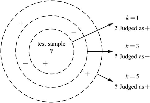
Figure 1 shows a diagram of a k-nearest neighbors classifier, with the dotted lines as the equidistant lines. Obviously, when k is taken different values, the classification results will be significantly different; on the other hand, if different distance measurement methods are used, the “nearest neighbors” found for a given test sample will also be different, which can result in substantially different classification results (Goldberger et al., 2005). This paper optimized the kNN classification model starting from the above two aspects to improve its accuracy and prediction ability. The main means was to introduce the modified nearest NCA algorithm and Bayesian hyperparameter tuning.

Figure 1

Figure 1. Diagram of k-Nearest Neighbors Classifier.

3.2 Iterative paramete updating strategy and convergence analysis of bayesian optimization process

Bayesian optimization is an effective method for hyperparameter tuning, involving an iterative process of parameter updating and convergence analysis to find the optimal solution. Here’s a detailed description of the iterative parameter updating strategy and convergence analysis in the Bayesian optimization process:

3.2.1 Iterative parameter updating strategy

The iterative parameter updating in Bayesian optimization follows these steps:

Step 1. Initialization:

Select an initial set of hyperparameters and evaluate them using the objective function (e.g., cross-validation score of a model).

Step 2. Build a Surrogate Model:

Use a probabilistic model like Gaussian Processes (GP) to approximate the objective function. This surrogate model learns the distribution of the objective function based on the evaluations made so far.

Step 3. Choose an Acquisition Function:

The acquisition function determines the next hyperparameter point to evaluate. Common acquisition functions include Expected Improvement (EI), Upper Confidence Bound (UCB), and Entropy Search.

Step 4. Optimize the Acquisition Function:

Find the hyperparameter point that maximizes the acquisition function. This point is chosen based on a trade-off between high predicted performance and high uncertainty.

Step 5. Evaluate New Hyperparameters:

Assess the objective function using the selected hyperparameter point and add the result to the existing dataset.

Step 6. Update the Surrogate Model:

Incorporate the new evaluation result into the surrogate model, then repeat steps 3 to 5 until a stopping criterion is met (such as reaching a maximum number of iterations or when improvements are no longer significant).

3.2.2 Convergence analysis

The convergence analysis of Bayesian optimization focuses on whether the algorithm can converge to the global optimum or its vicinity. The theoretical convergence of Bayesian optimization depends on several factors:

1. Accuracy of the Surrogate Model: If the surrogate model can accurately approximate the objective function, the algorithm is more likely to find the optimal solution.

2. Choice of Acquisition Function: Different acquisition functions lead to different search strategies. For example, Expected Improvement (EI) tends to look for improvements near regions that are already known to be good, while Upper Confidence Bound (UCB) places more emphasis on exploring unknown regions.

3. Balance Between Exploration and Exploitation: Bayesian optimization balances exploration (searching in areas with high uncertainty) and exploitation (searching in areas predicted to have high performance) through the acquisition function. A good balance can improve the speed and quality of convergence.

4. Stopping Criteria: Appropriate stopping criteria prevent overfitting and unnecessary computation. Common stopping criteria include reaching a maximum number of iterations, improvements falling below a certain threshold, or limitations on computational resources.

In practice, Bayesian optimization typically requires fewer iterations than grid search and random search to find a near-optimal set of hyperparameters, especially in high-dimensional search spaces. However, the convergence rate and final performance of Bayesian optimization are also influenced by the choice of surrogate model, acquisition function design, and initial point selection.

Overall, Bayesian optimization iteratively updates parameters and carefully designed acquisition functions to balance exploration and exploitation, effectively addressing hyperparameter tuning problems. Although its theoretical convergence may be difficult to guarantee in some cases, Bayesian optimization has proven to be a powerful and effective tool in practice.

3.3 Hyperparameter tuning

The process of identifying the best set of model parameters, including the nearest neighbor k, is called hyperparameter tuning. Two common parameter tuning methods are grid search and Bayesian optimization. Although grid search can thoroughly traverse a limited set of parameter value combinations to evaluate the objective function value and find the best model, it takes too long and is prone to the disaster of dimensionality. The Bayesian optimization algorithm (BOA) is based on Bayes’ theorem (Deng, 2019), the basic idea of which is to use all available information in previous evaluations to learn the form of the objective function, so as to find the minimum value of the complex non-convex function through few evaluations. This process is divided into two steps:

1) Use the probability model to represent the unknown objective function of the original model to be evaluated, continuously increase the volume of information and modify the prior through iteration. The probabilistic model established in this paper adopted the Gaussian process, which is highly flexible and scalable (Cui and Yang, 2018).

If X refers to the training set {x₁,x₂, … ,x_t}, f refers to the set of function values {f (x₁),f (x₂),…,f (x_t)} for an unknown function, θ refers to the hyperparameter. When there is observed noise and if the noise ε satisfies the independent and equally distributed Gaussian distribution p(ε) = (0, σ²), the marginal likelihood distribution can be obtained as follows:

$\mathit{p}\left(\mathit{y}|\mathit{X},\mathit{\theta }\right)=\int \mathit{p}\left(\mathit{y}|\mathit{f}\right)\mathit{p}\left(\mathit{y}|\mathit{X},\mathit{\theta }\right)\mathit{d}\mathit{f}$

By maximizing the marginal likelihood distribution through maximum likelihood estimation, θ_best is obtained, which is the optimal solution based on the observed values so far.

2) Choose an acquisition function to construct a utility function from the posterior model, and determine the next sampling point. In this paper, the common expectation improvement function was used to accomplish this goal by finding the maximum expected increment under the current best situation:

$\mathit{\alpha }\left(\mathit{\theta }|\mathit{\mu },\mathit{\sigma }\right)=\mathit{E}\left[\mathit{max}\left(\mathbf{0},\mathit{f}\left(\mathit{\theta }\right)-\mathit{f}\left({\mathit{\theta }}_{\mathit{b}\mathit{e}\mathit{s}\mathit{t}}\right)\right)\right]$

where, μ is the predicted mean function of the prior model, and σ is the predicted variance function of the prior model.

In each iteration, the Bayesian hyperparameter tuning algorithm first selects the next most promising evaluation point x_t according to the maximum acquisition function, then evaluates the objective function value f (x_t) based on the selected evaluation point, and finally adds the newly obtained observation value to the historical observation set and updates the probability proxy model to prepare for the next iteration.

The NCA-KNN model reduces computational complexity by dimensionality reduction, Feature Extraction, efficient distance calculation, adaptive K values, clustering-based search, .and utilizing of KD trees. Achieving a balance between computational efficiency and classification accuracy involves several strategies, including parameter tuning, hybrid approaches, intelligent data sampling, regular model validation.

4 Transformer fault diagnosis based on NCA and kNN

4.1 Diagnosis process

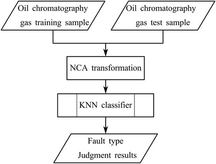
The transformer fault diagnosis process based on kNN is shown in Figure 2.

Figure 2

Figure 2. Flowchart of the fault diagnosis based on KNN.

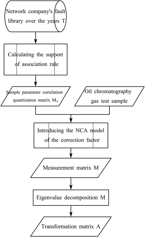
NCA transformation refers to the mapping of the transformer fault samples using the output results (metric matrix) of the NCA model. The training process of NCA is shown in Figure 3, and the improved NCA algorithm proposed in this paper was used in the process.

Figure 3

Figure 3. Flowchart of the NCA training.

In addition, the performance of the model is highly dependent on the selection of hyperparameters (number of NCA trainings and kNN nearest neighbor parameter k). In this paper, the Bayesian Optimization Algorithm (BOA) (Deng, 2019) was used to optimize them to enhance the diagnostic performance of the model. Since the goal of BOA is to find the minimum value of a complex non-convex function, this paper sets its objective function as the negative value of the fault classification accuracy of the test set.

4.2 Selection of initial value of metric matrix

In the NCA algorithm, the metric matrix M is usually initialized by random assignment. In order to reduce the number of NCA training times and improve the training efficiency, this paper quantified the correlation of each parameter of transformer fault samples into a multidimensional array through the support calculation method of the association rule (Li et al., 2013), thereby forming the initial metric matrix M₀ of NCA as a whole.

The association rule is to find the correlation between different items appearing in the same event. It is supposed that I = {i₁,i₂,i₃, …, i_B} is a finite item set consisting of B items to be studied and a transaction database T = {T₁,T₂,T₃, … ,T_D} is given. If, for a subset P of I, a transaction T ⊃ P exists, then the transaction is said to contain P. There are two basic metrics for measuring the association rule: support and confidence. Since the metric matrix is symmetric, this paper used support to measure the correlation between parameters.

Support S is defined as the probability that P and Q appear in a transaction at the same time, and is estimated by the proportion of the number of transactions in which P and Q appear in the sample data set I in the total number of transactions:

$\mathit{S}\left(\mathit{P}\to \mathit{Q}\right)=\mathit{S}\left(\mathit{Q}\to \mathit{P}\right)=\frac{\left|\mathit{T}(\mathit{P}\vee \left.\mathit{Q})\right|\right.}{\left|\mathit{T}\right|}$

In the above formula, |T(P˅Q)| indicates the number of transactions that contain both P and Q; |T| indicates the total number of transactions.

In this paper, the total number of transactions T is the total number of all oil chromatography sample databases, and the item set i_b = {the value of the bth gas parameter is greater than the average of the parameters in the database}. In this way, the support of each gas parameter of the oil chromatography was calculated respectively, and finally, the initial metric matrix M₀ was obtained.

5 Case analysis

5.1 Oil chromatography data

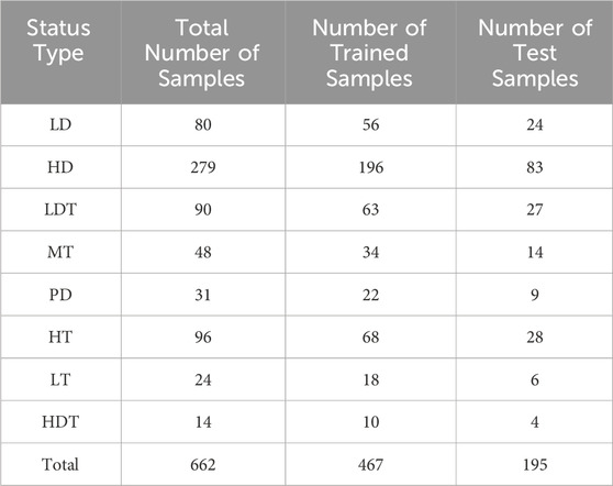
The method proposed in this paper was discussed by using a data set of 662 samples, which consisted of the fault case library of a certain power grid company and the oil chromatography data in the published literature in the related field as an example (Li and Tao, 2024). Each sample in the library contains eight characteristic parameters: H₂, CH₄, C₂H₂, C₂H₄, C₂H₆, CO, CO₂ and total hydrocarbon content. The faults were divided into eight types: low energy discharge (LD), high energy discharge (HD), low energy discharge and overheating (LDT), partial discharge (PD), medium temperature overheating (MT) (300°C < T < 700°C), low temperature overheating LT (T < 300°C), high energy discharge and overheating (HDT) and high temperature overheating (HT) (T > 700°C). Among the 662 samples, 468 sets of data were taken as training sets and the remaining 194 sets of data were taken as test sets for parameter training and generalization test of the model. The number distribution of data set samples is shown in Table 1.

Table 1

Table 1. Sample distribution in training and testing dataset.

5.2 Data preprocessing

In actual oil chromatography fault samples, the values of some characteristic gases grow exponentially, which makes the distance between fault samples of the same type larger, and has a greater influence on the kNN algorithm based on metric distance classification. Besides, in order to reduce the influence of the absolute value fluctuation of each characteristic gas concentration in different cases, the normalization method of the following formula was adopted in this paper to perform numerical scaling with a target interval of (0,1]:

${\mathit{x}}^{\prime }={\mathit{log}}_{\left(\mathit{max}\mathit{x}+\mathbf{1}\right)}\left(\mathbf{1}+\mathit{x}\right)$

The logarithmic transformation in the formula can stretch the data distribution within the lower amplitude range and compress the data distribution within the higher amplitude range, making the distribution of fault data as uniform as possible and reducing the influence of extreme values on the classification results to a certain extent. The normalized sample data were stacked row by row, generating a training set matrix of 467 × 8 and a test set matrix of 195 × 8, respectively.

5.3 Initial value of metric matrix

The initial value M₀ of the metric matrix in this example was obtained by calculating the support of each gas parameter in the oil chromatography using the method proposed in this paper, based on the oil chromatography data of 1,104 fault samples from a certain network company over the years. With H₂ and CH₄ as examples, there are 37 samples whose values of the two parameters are simultaneously greater than the corresponding average. The calculation process is as follows: S(CH₄→H₂) = S(CH₄←H₂) = 37/1,104 = 0.0335,145. Similarly, each parameter was calculated and an item of 8-dimensional data was finally obtained, as shown in Table 2.

Table 2

Table 2. Quantitative Correlation matrix of oil chromatography sample parameters (%).

5.4 Optimization of sample imbalance

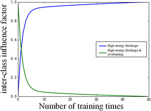
From the data volume distribution in Table 1, it can be seen that the ratio of high-energy discharge with the largest number of samples and the high-energy discharge and overheating with the smallest number of samples in the training samples was 19.6:1, indicating a serious imbalance. Figure 4 shows the change of the inter-class influence factors of high-energy discharge samples and high-energy discharge overheating samples with the number of training times during the training of the traditional NCA model. For the convenience of comparison, the inter-class influence factors were scaled according to the maximum and minimum values in the target interval [0,1]. The actual ratio of the two is about 400:1.

Figure 4

Figure 4. The curves of HD and HDT’s inter-class influence factor.

As can be seen from Figure 4, with the training of NCA, the inter-class influence factor of high-energy discharge samples gradually increased, while the opposite is true for high-energy discharge and overheating, and the optimization of the objective function tended to favor large-class data.

The improved NCA model proposed in this paper was used to train the fault samples, and the inter-class influence factors of high-energy discharge samples as well as high-energy discharge and overheating samples change with the number of training times as shown in Figure 5.

Figure 5

Figure 5. The curve of HD and HDT’s inter-class influence factor.

It can be seen that with the method proposed in this paper, the inter-class influence factors of the two gradually increased with training, and the problem of small samples being ignored due to sample imbalance in Figure 4 was controlled to a certain extent.

5.5 Hyperparameter tuning

The hyperparameter tuning results of this case obtained according to the hyperparameter tuning method in this paper, are shown in Figure 6.

Figure 6

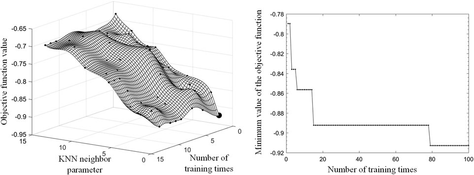
Figure 6. Hyper Parameter Tuning Process and Results. (A) Objective function fitting the distribution model; (B) Minimum change curve of the objective function.

Figure 6A shows the objective function distribution model obtained based on the historical observation set, where the slightly smaller dots indicate the sampled observation points, and the slightly larger dots are the best-estimated feasible points, that is, the sampling points with the lowest function values estimated by the latest model. Figure 6B shows a curve indicating the change of the minimum value of the historical observation set of the objective function with the number of iterations during the training process. It can be seen that the model trained with the optimized hyperparameters saw increased fault classification accuracy on the test set and enhanced model diagnostic performance.

If the traditional grid search method is used, that is, a finite set of parameter value combinations is thoroughly traversed to evaluate the objective function value, the performance comparison is shown in Table 3. The results show that the fault classification accuracy of the test set of the model trained with hyperparameters optimized by the Bayesian optimization algorithm is slightly lower than the result of the grid search, but significantly higher than the accuracy before optimization. This indicates that the BOA algorithm can effectively optimize the hyperparameters of the model proposed in this paper, and the effect is as expected. Also, the computational time cost of the Bayesian optimization algorithm was reduced by about 19.32s compared with the grid search, which indicates a significant effect.

Table 3

Table 3. Performance comparison of hyper parameter optimization methods.

5.6 Fault diagnosis analysis and comparison

The transformer faults were diagnosed with the method proposed in this paper. For comparison, other traditional methods (three-layer BP-based neural network, support vector machine (SVM) with radial basis kernel function (RBF), kNN and uncorrected NCA-kNN) were also used in this paper. In addition, for a fair comparison, the same Bayesian optimization algorithm was used to optimize the hyperparameters of each model, with the learning rate set to 0.001 and the accuracy set to 1e-5. At the same time, SVM used inter-class imbalanced weight adjustment during training.

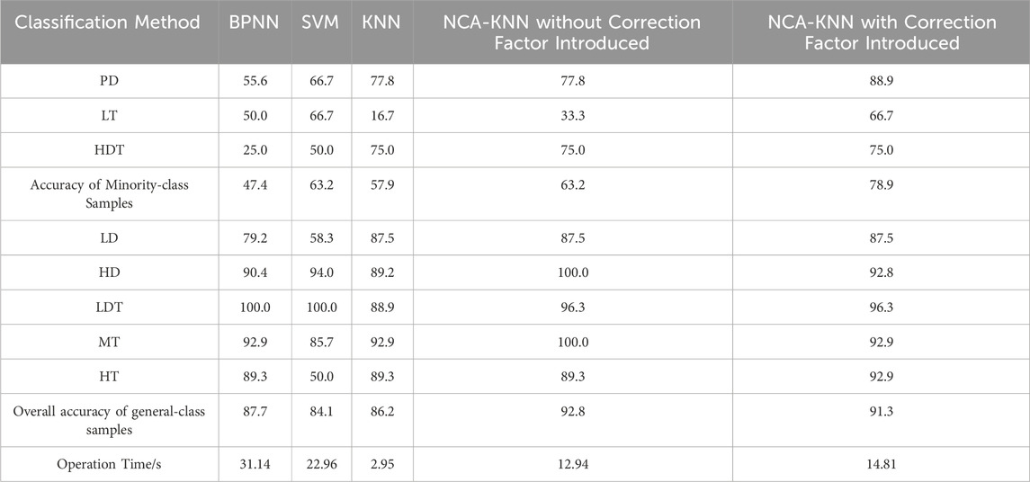
The diagnostic accuracy and running time were compared. According to the number of fault samples, partial discharge (PD), low temperature overheating (LT) and high energy discharge and overheating (HDT) were classified as minority samples. The diagnostic results are shown in Table 4.

Table 4

Table 4. Comparison of diagnostic accuracy of each model on testing dataset.

By analyzing the data in the table, it is known that the traditional NCA-kNN had the best performance among the five methods from the perspective of overall diagnostic accuracy, reaching 92.8%, and the improved NCA-kNN model in this paper was secondary, with an accuracy of 91.3%.

From the perspective of the operation time of each model, the two NCA-kNN models achieved performance superior to that of BPNN and SVM algorithms in only about 1/2 to 1/3 of the time.

From the perspective of the classification accuracy of minority samples, that is, the recall rate, the NCA-kNN model with the correction factor proposed in this paper had the best performance, reaching 78.9%. Besides, it was not less than 60% for any fault type, more stable than that of other models. The BPNN model did not adopt any method for training imbalanced data, the accuracy of minority-class samples was only 47.4%, which was the worst performance among all models. SVM adopted the weight adjustment of inter-class imbalance and slightly reduced the performance difference between minority-class samples and majority-class samples, but its effect was still not ideal.

In the k-nearest neighbor (k-NN) algorithm, by adjusting the distance metric or using a weighted voting mechanism to introduce a correction factor, and SVM by introducing weights in the loss function as a correction factor, the model can pay more attention to minority class samples during training, thereby improving the classification performance of minority classes.

It can be seen that the improved NCA-kNN model with the correction factor proposed in this paper had an overall accuracy rate of only 1.5% lower than the best value among all the models. Also, its minority-class sample accuracy was improved by 15%–31% compared with other models. This indicates that the model had a good recognition and diagnosis capability for minority-class samples while ensuring the overall classification performance and operating efficiency.

6 Conclusion

In this paper, an NCA-kNN fault diagnosis model with a correction factor was constructed and its application in power transformer fault diagnosis was analyzed and introduced. Finally, the following conclusions were drawn through comparative analysis:

(1) By introducing a correction factor into the objective function of the NCA algorithm, the issue of small samples being ignored when optimizing the objective function due to sample imbalance was controlled to a certain extent;

(2) The correlation between the parameters of the oil chromatography samples was discovered by using the association rule, and the quantified results were used as the initial values for NCA algorithm training. Compared with random initialization, the number of NCA training times was smaller, and the training efficiency of NCA was improved. After NCA training, the number of dimensions of the sample decreased, which reduced the distance calculation time of the KNN classification network;

(3) The Bayesian optimization algorithm was used to tune the hyperparameters of the diagnostic model proposed in this paper. The diagnostic accuracy was improved by 11% compared with the unoptimized model, and the time cost was reduced by 19.32s compared with the common grid search. The operation efficiency optimization effect is obvious;

(4) Through comparison with other machine learning diagnosis methods, the transformer diagnosis model proposed in this paper can improve the accuracy of minority class samples by at least 15%. It only takes about half the processing time for the model to achieve an overall accuracy that is better than that of traditional machine learning algorithms. Besides, the model has good performance in overall classification, operation efficiency and classification of minority class samples.

Data availability statement

The original contributions presented in the study are included in the article/supplementary material, further inquiries can be directed to the corresponding author.

Author contributions

JC: Conceptualization, Data curation, Methodology, Project administration, Writing–original draft. YW: Formal Analysis, Investigation, Writing–original draft. LK: Software, Visualization, Writing–original draft. YC: Validation, Writing–original draft. MC: Funding acquisition, Resources, Writing–original draft. QC: Writing–review and editing. GS: Supervision, Writing–review and editing.

Funding

The author(s) declare that financial support was received for the research, authorship, and/or publication of this article. This work was supported by Science and Technology Project of China Southern Power Grid Co. Ltd. (No: GDKJXM20220236/030111KK52220019).

Conflict of interest

Authors JC, YW, LK, YC, and MC were employed by Guangzhou Power Supply Bureau of Guangdong Power Grid Co. Ltd.

The remaining authors declare that the research was conducted in the absence of any commercial or financial relationships that could be construed as a potential conflict of interest.

The authors declare that this study received funding from China Southern Power Grid Co. Ltd. The funder provided additional resources in the form of equipment and an expert consultant for the data analysis phase of the study.

Publisher’s note

All claims expressed in this article are solely those of the authors and do not necessarily represent those of their affiliated organizations, or those of the publisher, the editors and the reviewers. Any product that may be evaluated in this article, or claim that may be made by its manufacturer, is not guaranteed or endorsed by the publisher.

Supplementary material

The Supplementary Material for this article can be found online at: https://www.frontiersin.org/articles/10.3389/fenrg.2024.1500548/full#supplementary-material

References

Bai, C., Gao, W., Jin, L., et al. (2013). Integrated diagnosis of transformer faults based on three-layer bayesian network. High. Volt. Eng. 39 (2), 330–335.

Google Scholar

Cover, T. M., and Hart, P. E. (1967). Nearest neighbor pattern classification. IEEE Trans. Inf. Theory 13, 21–27. doi:10.1109/tit.1967.1053964

CrossRef Full Text | Google Scholar

Cui, J., and Yang, B. (2018). Survey on bayesian optimization methodology and applications. J. Softw. 29 (10), 3068–3090.

Google Scholar

Dai, J., Song, H., Yang, Y., et al. (2018). Dissolved gas analysis of insulating oil for power transformer fault diagnosis based on ReLU-DBN. Power Syst. Technol. 42 (2), 658–664.

Google Scholar

Deng, S., Chen, Y., Sheng, G., and Jiang, X. (2019). Hyper-parameter optimization of CNN based on improved Bayesian optimization algorithm. Appl. Res. Comput. 36 (7), 1984–1987.

Google Scholar

Duval, M. (1989). Dissolved gas analysis: it can save your transformer. IEEE Electr. Insul. Mag. 5 (6), 22–27. doi:10.1109/57.44605

CrossRef Full Text | Google Scholar

Fan, Y. (2023). “Research on transformer Fault Diagnosis method based on deep learning algorithm optimization,” in 2023 international conference on electronics and devices, computational science (ICEDCS) (Marseille, France: IEEE), 276–281.

CrossRef Full Text | Google Scholar

Goldberger, J., Roweis, S., Hinton, G., et al. (2005). Neighbourhood component analysis. Adv. Neural Inf. Process. Syst. 17, 513–520.

Google Scholar

Gu, K., Guo, J., and Salakhutdinov, R. (2014). Transformer fault diagnosis method based on compact fusion of fuzzy set and fault tree. High. Volt. Eng. 40 (5), 1507–1513.

Google Scholar

He, H., and Garcia, E. A. (2008). Learning from imbalanced data. IEEE Trans. Knowl. Data Eng. 9, 1263–1284.

Google Scholar

Li, R., and Hu, Y. (2004). A density-based method for reducing the amount of training data in KNN text classification. J. Of Comput. Res. Dev. 41 (4), 539–545.

Google Scholar

Li, Y., and Shu, N. (2016). Transformer fault diagnosis based on fuzzy clustering and complete binary tree support vector machine. Trans. China Electrotech. Soc. 31 (4), 64–70.

Google Scholar

Li, W., and Tao, W. (2024). “Research on prediction model of dissolved gas concentration in transformer oil based on deep learning algorithm,” in 2024 IEEE 2nd international conference on sensors, electronics and computer engineering (ICSECE) (Jinzhou, China: IEEE), 1459–1463.

CrossRef Full Text | Google Scholar

Li, L., Zhang, D., Xie, L., et al. (2013). A condition assessment method of power transformers based on association rules and variable weight coefficients. Proc. CSEE 24, 152–159.

Google Scholar

Li, W., Li, Q., Liu, Z., Yu, B., and Lin, F. (2019). Salient object detection using weighted k-nearest neighbor linear blending. J. Electron. and Inf. Technol. 41 (10), 2442–2449.

Google Scholar

Ling, H., Liu, J., and Li, Z. (2012). Troubleshooting of transformer faults by chromatogram analysis of transformer oil. Hydraulics Pneumatics and Seals 32 (5), 46–50.

Google Scholar

Lu, T., Ma, H., Zhang, Y., et al. (2024). “Fault diagnosis of power transformer based on KPCA-RF,” in 2024 9th international conference on intelligent computing and signal processing (ICSP) (Xian, China: IEEE), 1698–1702.

CrossRef Full Text | Google Scholar

Rogers, R. R., and Qin, X. (1978). IEEE and IEC codes to interpret incipient faults in transformers, using gas in oil analysis. IEEE Trans. Electr. Insulation. 5, 349–354. doi:10.1109/tei.1978.298141

CrossRef Full Text | Google Scholar

Tejaswini, N. P., Riad Al-Fatlawy, R., et al. (2024). “Fault detection in smart grids by hybrid generative adversarial networks with neuro fuzzy algorithm,” in 2024 international conference on intelligent algorithms for computational intelligence systems (IACIS) (Hassan, India: IEEE), 1–4.

Google Scholar

Wang, C., Pan, Z., Ma, C., Malathy, V., Kirthiga, N., and Mudunuri, E. C. V. S. (2012). Classification for imbalanced dataset of improved weighted KNN algorithm. Comput. Eng. 38 (20), 160–163.

Google Scholar

Wang, K., Li, J., Zhang, S., Dong, L., and Zhang, T. (2016). New features derived from dissolved gas analysis for fault diagnosis of power transformers. Proc. Chin. Soc. Electr. Eng. 36 (23), 6570–6578.

Google Scholar

Wu, M., Wang, G., Liu, H., Sun, J., Wang, J., Gao, F., et al. (2022). “Research on transformer Fault Diagnosis based on SMOTE and random forest,” in 2022 4th international conference on electrical engineering and control technologies (CEECT) (Shanghai, China: IEEE), 359–363.

CrossRef Full Text | Google Scholar

Zhang, X., Zhou, Mi., and Geng, G. (2010). Research on improvement of Bagging Chinese text categorization classifier. J. Of Chin. Comput. Syst. 31 (2), 281–284.

Google Scholar

Zhou, H. T., Chen, J., Dong, G. M., Wang, H. C., and Yuan, H. D. (2016). Bearing fault recognition method based on neighborhood component analysis and coupled hidden Markov model. Mech. Syst. Signal Process. 66/67, 568–581.

Google Scholar