A two-phase robust comprehensive optimal scheduling strategy for regional distribution network based on multiple scenarios

With the increasing integration of renewable energy sources, the optimization of distribution networks has become a critical challenge to ensure sustainable and reliable energy supply. In this paper, a robust comprehensive optimization (RCO) strategy based on multi-scenarios is proposed to manage the uncertainty of distributed power supply and load in regional distribution networks, for making up for the shortcomings of existing methods in multi-scenario integrated energy optimization of distribution networks. Firstly, the development of a holistic model that concurrently considers constraints related to wind power, photovoltaics (PVs), gas turbines (GTs), energy storage systems, reactive power compensation, and carbon dioxide (CO₂) emissions, ensuring a comprehensive approach to network management. Then, the application of Latin Hypercube Sampling (LHS) for scenario generation, combined with an adaptive K-means clustering approach using the elbow method (EM), which results in the creation of highly representative prototypical scenarios. In addition, the imposition of 1-norm and ∞-norm constraints on the probability confidence intervals for scenario distribution, provides a rigorous framework for addressing uncertainty in energy scenarios. Furthermore, a novel two-phase decomposition model based on the box decomposition algorithm will be introduced to handle the temporal dependencies between energy storage and unit commitment, optimizing both operational costs and system flexibility. Using the column and constraint generation (C&CG) algorithm, the proposed complex optimization problem has been solved comprehensively. Finally, the validation of the model using the IEEE 33-note system based on the Matlab/Simulink platform from four regional distribution networks, demonstrates that the proposed method can effectively improve the practicability, reduce the clustering error, enhance the robustness, and have better scene representation.

1 Introduction

In the wake of the global energy structure’s metamorphosis and the relentless progress of new energy technologies, distributed generation (DG) has attracted widespread scrutiny and undergone rapid proliferation on a global scale (Cheng et al., 2023). Nonetheless, this has also brought to the fore an increasingly prominent tension between the unpredictability of DG output and the flexibility of the power grid, presenting immense challenges to the security of the worldwide electrical system (Li et al., 2021). Under conventional centralized power management systems, the distribution of system load and power generation is orchestrated and allocated by a central control mechanism, thereby ensuring a higher degree of operational stability (Saaklayen et al., 2024). However, with the integration of DG, the power sources within the grid have become more dispersed, and the output of DG is subject to the vagaries of weather and environmental factors, thereby exhibiting considerable uncertainty (Zhang et al., 2020). This unpredictability complicates the forecasting of the power grid’s operation, substantially impacting its flexibility and stability, and consequently placing increased demands on system security (Mahdavi et al., 2023). Thus, the conundrum of reconciling the uncertainty of DG output with the grid’s flexibility to enhance the security of the global energy infrastructure has become a paramount challenge for the international energy sector (Wang et al., 2020).

Randomized optimization (Wada and Fujisaki, 2015) and robust optimization (RO) (Margellos et al., 2014) are the two principal approaches to addressing the uncertainty in DG output, yet its own challenges beset each: the former with issues of statistical optimality, where decision accuracy is contingent upon the quantity of statistical data, and the latter with problems of conservatism. The literature Zhang et al., (2018) introduces a method to evaluate distribution systems’ maximum hosting capacity (MHC) for DG, considering the optimal operation of on-load tap changers and static var compensators under uncertain conditions. However, the method may not account for all MHC scenarios and does not address robustness against data errors. The literature Wang et al. (2016) examined the use of fractional order (FO) automatic generation control for controlling power system frequency oscillations in a hybrid distributed energy system. Compared to optimal solutions, its parameters are tuned using RO with particle swarm optimization (PSO) variants. However, the method may face challenges in accurately approximating FO operators and could be computationally intensive, potentially leading to a large number of function evaluations despite the archival-based strategy. The literature Abboud et al. (2016) suggests a frequency control scheme for electric vehicles (EVs) that adjusts operational modes based on grid frequency thresholds, aiming to stabilize the grid during supply-demand imbalances. The method’s limitations include the requirement for accurate threshold determination and potential vulnerability to variations in EV participation rates. The asynchronous distributed alternating direction method of multipliers (ADMM) algorithm investigated in the literature Moghadam et al. (2016) offers flexibility in handling synchronization constraints and random local failures, making it suitable for applications like the direct-current optimal power flow in power transmission networks. Whereas, the algorithm may encounter challenges in maintaining convergence due to substantial network delays or communication failures. The literature Yuan et al. (2016) proposed probability-weighted RO method for long-term DG planning in micro-grids effectively handles the uncertainty of intermittent sources like wind turbines. The method provides full operational robustness. However, it is computationally intensive, which may limit its practicality for large-scale systems or in resource-constrained environments.

Distributed robust optimization (DRO) (Bürger et al., 2014) effectively mediates the tension between randomized optimization and RO, emerging as a potent strategy for coping with uncertainty. By leveraging the 1-norm (Barni, 1997) and ∞-norm (Campo and Morari, 1986) to circumscribe confidence intervals, this method circumvents the complexities of non-deterministic polynomial problems, thus simplifying the solution process. To date, this approach has garnered preliminary application in areas such as energy storage management (Darivianakis et al., 2017), integrated energy system dispatch (Zhang et al., 2021), and transmission network planning (Bagheri et al., 2017). Such applications have demonstrated that DRO holds great promise, offering precise and robust solutions in the management of DG output uncertainty. The literature Wang et al. (2021) proposes a DRO approach for hybrid AC/DC regional distribution networks, which simultaneously minimizes network losses, voltage deviations, and operational costs, enhancing safety, flexibility, and economy. However, its computational requirements should be considered for large-scale systems, and the method’s effectiveness may be sensitive to the selection of parameters and the accuracy of input data. The literature Wang et al. (2022) proposed a transactive energy sharing (TES) approach for micro-grids aims to minimize social costs while addressing uncertainties in renewable generation and loads. The TES problem is solved using ADMM, with adaptive RO and column and constraint generation (C&CG) managing uncertainties. An alternating uncertainty update procedure is introduced to improve ADMM convergence. Nevertheless, the method may be computationally intensive, especially for large-scale micro-grids, and its performance could be sensitive to parameter selection and input data accuracy.

To address the deficiencies inherent in the aforementioned research, this paper constructs a robust comprehensive optimization (RCO) model that amalgamates wind, solar, load, and storage, taking into account the network architecture. By manipulating the network topology and the output of various distributed generators, the model ascertains the most cost-effective solution while satisfying system security constraints. Considering the dynamic constraints imposed by energy storage, turbines, and topology on the solution efficiency, the variables are decoupled into two categories for resolution: the continuous variables such as turbines and energy storage are designated as the first category, whereas the discrete variables associated with network topology are classified as the second. The box decomposition algorithm Ratschan (2002) is applied to regional distribution network optimization, with the first category of variables undergoing a two-phase resolution process. Phase 1 introduces dynamic constraints, and the original multi-period optimization problem is decomposed into several single-period optimization problems in Phase 2. The resultant first-category variables are then incorporated into the dynamic reconstruction model, with a heuristic rule-based particle swarm algorithm employed to determine the second-category variables. The 1-norm and ∞-norm are utilized to identify the probability distribution under the worst-case scenario. The RCO model uses the C&CG algorithm and intelligent algorithms for iterative solutions.

The content of this paper is organized as follows: Second 2 analyzes the scene generation process of RCO method, and gives the design steps of data sampling and scenario clustering; Section 3, the optimization model of regional distribution network is presented, the objective function and constraint conditions are given in two-phase, and the random optimization model is proposed based on the dynamic reconstruction mechanism. In Section 4, the detailed solving steps of the proposed model are given based on the classification mechanism of the main problem and sub-problem. In Section 5, the performance of the proposed model is analyzed with an IEEE 33-node example system to verify the superior performance of the two-phase RCO, comprehensive optimal scheduling model for solving the integrated energy system of the regional distribution network.

2 Integrated energy system scenario generation

The RO approach predicated on scenario probability distributions exacts a premium on both the quantity and the precision of scenario generation. In light of the inter dependencies among load, wind power, and photovoltaic (PV) output, which are influenced by geographical and anthropogenic factors within real-world scenarios, this paper employs Latin hypercube sampling (LHS) (Shin et al., 2009) to treat the initial sample data for correlation, thereby yielding sample datasets with defined correlation coefficients. Subsequently, the elbow method (EM) (Liu and Deng, 2021) is utilized to ascertain the most appropriate number of scenarios, followed by the application of an enhanced K-means clustering technique (Sinaga and Yang, 2020) to derive more representative prototypical scenarios.

2.1 Data sampling

The distribution of errors in random variables significantly impacts the rationality of random scenario generation under multiple scenarios. The kernel density estimation method (Hu et al., 2017) can validate that the error distributions of load and DG outputs conform to a normal distribution. LHS accomplishes a stratified sampling process, uniformly and comprehensively covering the distribution range of variables, encompassing both sampling and correlation control.

2.1.1 Sampling process

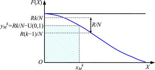
The essence of sampling is to divide the value range of the distribution function into N equal parts without altering the original density function, then to apply inverse function transformations based on the probability density function to the sampling values of each part, ultimately yielding the sampling results. The specific sampling procedure is shown in Figure 1. The detailed steps are as follows:

Step 1: It is presupposed that there are M random variables, each requiring N samples to generate an M×N order sample matrix denoted as X_MN:

${\mathit{X}}_{MN}=\left[\begin{array}{cccc}{x}_1^1& x_1^2& \cdots & x_1^N\\ x_2^1& x_2^2& \cdots & x_2^N\\ ⋮& ⋮& & ⋮\\ x_M^1& x_M^2& \cdots & x_M^N\end{array}\right](1)$

Step 2: The F(X) represents the probability density function of X, which is a normal distribution function. To facilitate the inversion of the function, F(X) is halved at its median point, and then sampling is conducted separately for the left and right halves.

Step 3: Assuming that the sampling result set of the M-th random variable is X_M = {x_M¹, x_M², …, x_M^k, …, x_M^N}, with the value domain of the normal distribution function being [0, R], the interval is divided into N non-overlapping sub-intervals based on the required sample size N. The k-th sampling result y_M^k obtained by random sampling within each interval according to a uniform distribution is as follows:

$y_M^k=\frac{Rk}{N}-\mathrm{U}\left(0,1\right)(2)$

where, U (0,1) denotes the uniformly distributed random sample values within the interval (0,1).

Step 4: Taking the inverse of the probability distribution function yields the actual sampling value x_M^k as follows:

$x_M^k=F^{-1}\left(y_M^k\right)(3)$

Step 5: Continuing to sample from the remaining sub-intervals, the steps above are repeated until the sampling process is complete.

Figure 1

Figure 1. Latin hypercube sampling process.

2.1.2 Correlation control method

Among the methods for correlation control, the Cholesky decomposition method (Hakkarinen et al., 2015) is widely utilized due to its computational simplicity. The steps are as follows:

Step 1: A random N×M matrix ANM is generated, which has the exact dimensions the original sampled data X_NM. N and M represent the number of variables and the number of samples drawn for each variable, respectively.

Step 2: Calculate the correlation coefficient matrix R_A between the row vectors of matrix ANM. Perform Cholesky decomposition on R_A to obtain a non-singular lower triangular matrix Q, and then can calculate the matrix D by the relationship as D = Q⁻¹A.

Step 3: The correlation matrix of the input variable is denoted as R_set. Perform the Cholesky decomposition on R_set to obtain the lower triangular matrix Q_set, and then calculate D_set = Q_setD.

Step 4: Subsequently, rearrange the elements of each row in matrix A according to the magnitude of the corresponding elements in D_set, resulting in a novel matrix A_set. By reordering the original data matrix in accordance with A_set, the ultimate sample matrix X_set is derived. At this juncture, the correlation matrix of X_set conforms to the predetermined correlation coefficient matrix.

2.2 Scenario clustering

2.2.1 Determine the number of clusters

As the number of clusters increases, the resulting scenarios more closely approximate the probability distribution of random variables. However, an excessively high number of clusters can compromise the computational efficiency of DRO models. Therefore, it is imperative to determine the most appropriate number of clusters based on the intrinsic characteristics of the data. The EM, renowned for its simplicity and efficacy, has emerged as a prevalent algorithm for determining the optimal number of clusters.

The EM employs the ratio of intra-cluster average distance (nSE) to inter-cluster average distance (wSE) as an indicator to describe the clustering error (SE). As the number of clusters increases, the sample partition becomes more refined, and the cohesion within each cluster gradually improves, resulting in a smaller nSE. However, when the number of clusters becomes too large, wSE is also tiny, yet SE may not necessarily be small. Therefore, a smaller clustering distance is observed only when nSE is relatively tiny, and wSE is relatively large. When the number of clusters k is less than the actual number of clusters, as k increases, wSE does not change significantly, while nSE decreases sharply, leading to a substantial decrease in SE. When k reaches the number of clusters, the decrease in nSE diminishes, and wSE remains unchanged or may even decrease slightly. At this point, the reduction rate in SE slows down, forming an elbow-shaped curve in the relationship between SE and the number of clusters k. The value of k corresponding to the elbow point represents the number of clusters within the data. The model can be expressed as follows:

$SE=\frac{nSE}{wSE}(4)$

$nSE={\displaystyle \sum _{i=1}^k}\left({\displaystyle \sum _{ks\in {\delta }_i}}{\left|ks-m_i\right|}^2/kn\right)/k(5)$

$wSE={\displaystyle \sum _{i=1}^k}{\displaystyle \sum _{j=i+1}^k}{\left|m_i-m_j\right|}^2/\left(k\left(k-1\right)/2\right)(6)$

where, δ_i represents the i-th cluster, k_s denotes the samples within δ_i, m_i is the centroid of δ_i, which is the mean of the samples in δ_i, and k_n is the number of samples within δ_i.

2.2.2 Improved K-means clustering

The primary steps for determining the optimal number of clusters using the EM, in conjunction with an enhanced K-means clustering algorithm, are as follows:

Step 1: Set the number of clusters to k and randomly select a scenario as the first cluster centroid, denoted as K₁.

Step 2: Calculate the Euclidean distance (Schouhamer Immink and Weber, 2015) between the remaining scenarios and K₁. Select the scenario with the greatest distance as the second cluster centroid, K₂. Then, calculate the sum of distances from the remaining scenarios to the two cluster centroids, identifying the scenario with the maximum sum as the third cluster centroid, K₃. Continue this process iteratively to obtain k initial cluster centroids.

Step 3: Compute the distances between the remaining scenarios and each cluster centroid, assigning the scenarios to the nearest cluster centroid and recalculating the cluster centroids for each category.

Step 4: Define the sum of squared distances between each scenario and its assigned cluster centroid as the clustering error H. When the difference in clustering error H between two consecutive iterations falls below a certain convergence threshold, terminate the iteration process, output the cluster centroids from the final iteration, and otherwise return to Step 3.

3 Regional distribution network optimization model

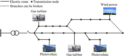
For a typical regional distribution network, as shown in Figure 2, in this paper, the box decomposition algorithm Ratschan (2002) is employed to decompose the variables into a two-phase solution process: dynamic constraints are incorporated into Phase 1, where the operational domains of microturbines and energy storage during each period are constrained, yielding the operational status and domain for each period of the unit, as well as the single-period operational domain for energy storage. In Phase 2, utilizing the results from Phase 1, the dynamic optimization problem across multiple time scales is decomposed into several single-scale optimization problems, from which the values of the first type of variables are obtained. Under the condition of known injection powers at each node, the PSO algorithm is used for dynamic reconstruction to solve for the second type of variables.

Figure 2

Figure 2. Schematic diagram of typical regional distribution network.

3.1 Model of phase 1

3.1.1 Objective function of the phase 1 model

The objective function for the first phase comprises the constant running cost of the gas turbine (GT), denoted as C_GT, the wind power generator operation cost C_WI, and the PV generator operation cost C_PV, as illustrated following:

$f_{P1}=\min \left(C_{\text{GT}}+C_{\text{WI}}+C_{\text{PV}}\right)(7)$

where

$\left\{\begin{array}{l}{C}_{\text{GT}}=C_S^{\text{GT}}{\displaystyle \sum _{t=1}^T}{\displaystyle \sum _{j\in {\mathrm{\Omega }}_{\text{GT}}}}{v}_{j,t}^{\text{GT}}{S}_{j,t}^{\text{GT}}\\ C_S^{\text{GT}}={\displaystyle \sum _{t=1}^T}{\displaystyle \sum _{j\in {\mathrm{\Omega }}_{\text{GT}}}}{u}_{j,t}^{\text{GT}}{c}_j^{\text{GT}}\\ S_{j,t}^{\text{GT}}={\alpha }_j^{\text{GT}}+{\beta }_j^{\text{GT}}\left[1-\exp \left(\frac{T_{j,t-1}^{\text{GT},\text{off}}}{{\tau }_j^{\text{GT}}}\right)\right]\forall t,\forall j\in {\mathrm{\Omega }}_{\text{GT}}\end{array}\right.(8)$

$\left\{\begin{array}{l}{C}_{\text{WI}}=C_S^{\text{WI}}\frac{r{\left(1+r\right)}^T}{{\left(1+r\right)}^T-1}{\displaystyle \sum _{j\in {\mathrm{\Omega }}_{\text{WI}}}}{N}_j^{\text{WI}}\\ C_S^{\text{WI}}={\displaystyle \sum _{j\in {\mathrm{\Omega }}_{\text{WI}}}}{u}_j^{\text{WI}}{c}_j^{\text{WI}}\end{array}\right.(9)$

$\left\{\begin{array}{l}{C}_{\text{PV}}=C_S^{\text{PV}}\frac{r{\left(1+r\right)}^T}{{\left(1+r\right)}^T-1}{\displaystyle \sum _{j\in {\mathrm{\Omega }}_{\text{PV}}}}{N}_j^{\text{PV}}\\ C_S^{\text{PV}}={\displaystyle \sum _{j\in {\mathrm{\Omega }}_{\text{PV}}}}{u}_j^{\text{PV}}{c}_j^{\text{PV}}\end{array}\right.(10)$

where, C_S^GT, C_S^WI and C_S^PV are the operating cost constants of GTs, wind power generators and PV generators, respectively; T represents the number of time periods; Ω_GT, Ω_WI and Ω_PV denotes the set of nodes containing GTs, wind power generators and PV generators; S_j,t^GT signifies the startup cost of the unit at node j during time period t; v_j,t^GT indicates the startup status of the unit at node j during time period t, where a value of 1 signifies that the unit has been started, and 0 indicates that it has not; u_j,t^GT denotes the operating status of the unit at node j during time period t, with a value of 1 indicating that the unit is running, and 0 indicating that it is not; α_j,t^GT and β_j,t^GT are the given constants for the unit at node j; τ_j,t^GT represents the time constant for the unit at node j; c_j^GT stands for the coefficient of the constant term for the operating cost of the unit at node j; and T denotes the consecutive downtime of the unit at node j during the time period t−1; r represents the discount rate; N_j^WI and N_j^PV respectively represent the number of wind power generators and PV generators installed at node j; u_j^WI and u_j^PV denote the operating status of wind power generators and PV generators of the unit at node j; c_j^WI and c_j^PV stand for the coefficient of constant terms for the operating cost of wind power generators and PV generators of the unit at node j.

3.1.2 Phase 1 constraints

Phase 1 of the unit constraint conditions encompasses the upper and lower bounds of the unit operating domain, the ramping constraints within the operating domain of the unit, and the minimum continuous running time constraint for the unit, which are respectively represented by (Equations 11–13), as shown in following:

$u_{j,t}^{\text{GT}}{P}_{j,t}^{\text{GT},\min }\le {\underset{\_}{P}}_{j,t}^{\text{GT}}\le {\overline{P}}_{j,t}^{\text{GT}}\le u_{j,t}^{\text{GT}}{P}_{j,t}^{\text{GT},\max }\forall t,\forall j\in {\mathrm{\Omega }}_{\text{GT}}(11)$

$\left\{\begin{array}{l}0\le t\left(u_{j,t}^{\text{GT}}-u_{j,t-1}^{\text{GT}}\right)+{\displaystyle \sum _{\gamma =t+1}^{\min \left(t-1+T_j^{\text{GT},\text{on}},T\right)}}{u}_{j,\gamma }^{\text{GT}}\le \min \left(t-1+T_j^{\text{GT},\text{on}},T\right)\forall t,\forall j\in {\mathrm{\Omega }}_{\text{GT}}\\ 0\le t\left(u_{j,t-1}^{\text{GT}}-u_{j,t}^{\text{GT}}\right)+{\displaystyle \sum _{\gamma =t+1}^{\min \left(t-1+T_j^{\text{GT},\text{off}},T\right)}}\left(1-u_{j,\gamma }^{\text{GT}}\right)\le \min \left(t-1+T_j^{\text{GT},\text{off}},T\right)\forall t,\forall j\in {\mathrm{\Omega }}_{\text{GT}}\end{array}\right.(12)$

$\left\{\begin{array}{c}\frac{{\underset{\_}{P}}_{j,t}^{\text{GT}}-{\underset{\_}{P}}_{j,t-1}^{\text{GT}}}{\Delta t}\le \Delta P_{j,t}^{\text{GT}+}\forall t,\forall j\in {\mathrm{\Omega }}_{\text{GT}}\\ \frac{{\overline{P}}_{j,t-1}^{\text{GT}}-{\overline{P}}_{j,t}^{\text{GT}}}{\Delta t}\le \Delta P_{j,t}^{\text{GT}-}\forall t,\forall j\in {\mathrm{\Omega }}_{\text{GT}}\end{array}\right.(13)$

where: P_j,t^GT,min and P_j,t^GT,max respectively denote the minimum and maximum technical output of the unit at node j during period t; ${\overline{P}}_{j,t}^{\text{GT}}$ and ${\underset{\_}{P}}_{j,t}^{\text{GT}}$ respectively signify the upper and lower limits of the production P_j,t^GT of the unit at node j during period t; T_j^GT,on and T_j^GT,off respectively represent the continuous operating time and the continuous downtime of the unit at node j; ΔP_j,t^GT+ and ΔP_j,t^GT− respectively indicate the maximum ramping up and ramping down power of the unit at node j during period t; and Δt denotes the time interval.

Phase 1 of the energy storage operational constraints includes the energy storage charging and discharging state constraints, the upper and lower bounds of the energy storage operating domain constraints, and the energy storage capacity constraints, which are respectively illustrated by (Equations 14–16) as follows:

$y_{j,t}^{\mathrm{E},\text{ch}}+y_{j,t}^{\mathrm{E},\text{dis}}\le 1\forall t,\forall j\in {\mathrm{\Omega }}_{\mathrm{E}}(14)$

$\left\{\begin{array}{l}0\le {\underset{\_}{P}}_{j,t}^{\mathrm{E},\text{ch}}\le {\overline{P}}_{j,t}^{\mathrm{E},\text{ch}}\le y_{j,t}^{\mathrm{E},\text{ch}}{P}_j^{\text{ch},\max }\forall t,\forall j\in {\mathrm{\Omega }}_{\mathrm{E}}\\ 0\le {\underset{\_}{P}}_{j,t}^{\mathrm{E},\text{dis}}\le {\overline{P}}_{j,t}^{\mathrm{E},\text{dis}}\le y_{j,t}^{\mathrm{E},\text{dis}}{P}_j^{\text{dis},\max }\forall t,\forall j\in {\mathrm{\Omega }}_{\mathrm{E}}\end{array}\right.(15)$

$\left\{\begin{array}{l}0\le {\displaystyle \sum _{v=1}^t}{\left(1-{\zeta }_j^{\mathrm{E}}\right)}^{t-v}\left[{\eta }_j^{\mathrm{E},\text{ch}}{\underset{\_}{P}}_{j,v}^{\mathrm{E},\text{ch}}-{\left({\eta }_j^{\mathrm{E},\text{dis}}\right)}^{-1}{\overline{P}}_{j,v}^{\mathrm{E},\text{dis}}\right]+E_j^{\mathrm{E}0}{\left(1-{\zeta }_j^{\mathrm{E}}\right)}^t\forall t,\forall j\in {\mathrm{\Omega }}_{\mathrm{E}}\\ {\displaystyle \sum _{v=1}^t}{\left(1-{\zeta }_j^{\mathrm{E}}\right)}^{t-v}\left[{\eta }_j^{\mathrm{E},\text{ch}}{\underset{\_}{P}}_{j,v}^{\mathrm{E},\text{ch}}-{\left({\eta }_j^{\mathrm{E},\text{dis}}\right)}^{-1}{\underset{\_}{P}}_{j,v}^{\mathrm{E},\text{dis}}\right]+E_j^{\mathrm{E}0}{\left(1-{\zeta }_j^{\mathrm{E}}\right)}^t\le E_j^{\mathrm{E},\max }\forall t,\forall j\in {\mathrm{\Omega }}_{\mathrm{E}}\end{array}\right.(16)$

where: Ω_E denotes the set of nodes containing energy storage systems; y_j,t^E,ch and y_j,t^E,dis respectively represent the charging and discharging states of the energy storage at node j during period t, which are 0–1 variables; ${\overline{P}}_{j,t}^{\mathrm{E},\text{ch}}$, ${\underset{\_}{P}}_{j,t}^{\mathrm{E},\text{ch}}$ and ${\overline{P}}_{j,t}^{\mathrm{E},\text{dis}}$, ${\underset{\_}{P}}_{j,t}^{\mathrm{E},\text{dis}}$ respectively indicate the upper and lower limits of the charging and discharging power $P_{j,t}^{\mathrm{E},\text{ch}}$ and $P_{j,t}^{\mathrm{E},\text{dis}}$ of the energy storage at node j during period t; $P_j^{\text{ch},\max }$ and $P_j^{\text{dis},\max }$ respectively signify the maximum charging and discharging powers of the energy storage at node j; E_j^E0 is the initial energy of the energy storage at node j; ζ_j^E represents the self-discharge efficiency of the energy storage at node j; η_j^E,ch and η_j^E,dis are the charging and discharging efficiencies of the energy storage at node j, respectively; and E_j^E,max denotes the maximum storage energy capacity of the energy storage at node j.

3.2 Model of phase 2

3.2.1 Objective function of the phase 2 model

The objective function for Phase 2, as represented by (Equation 17), encompasses the operating cost of the GT unit, C_fuel; the aging cost of the energy storage system (ESS), C_dge; the network loss cost, C_Ploss; the curtailment cost of wind and solar energy, C_Dlos; the cost of purchasing electricity from the main grid, C_grid; and the carbon emissions penalty cost, C_CO2.

$f_{P2}=\min \left(C_{\text{fule}}+C_{\text{dge}}+C_{\text{Ploss}}+C_{\text{Dloss}}+C_{\text{grid}}+C_{\text{CO}2}\right)(17)$

where,

$C_{\text{fule}}={\displaystyle \sum _{t=1}^T}{\displaystyle \sum _{j\in {\mathrm{\Omega }}_{\text{GT}}}}\left[a_j^{\text{GT}}{\left(P_{j.t}^{\text{GT}}\right)}^2+b_j^{\text{GT}}{P}_{j,t}^{\text{GT}}\right](18)$

$\left\{\begin{array}{l}{C}_{\text{dge}}={\displaystyle \sum _{t=1}^T}{\displaystyle \sum _{j\in {\mathrm{\Omega }}_{\mathrm{E}}}}\left[g_j^{\text{dge}}\left(P_{j.t}^{\mathrm{E},\text{ch}}+P_{j.t}^{\mathrm{E},\text{dis}}\right)\right]\\ g_j^{\text{dge}}=\frac{C_j^{\mathrm{E}}}{2B_j^{\mathrm{E}}\left(Q_j^{\mathrm{E}}\right)E_j^{\mathrm{E},\max }{Q}_j^{\mathrm{E}}}\forall t,\forall j\in {\mathrm{\Omega }}_{\mathrm{E}}\end{array}\right.(19)$

$\left\{\begin{array}{l}{C}_{\text{Ploss}}=C_{\mathrm{L}}{\displaystyle \sum _{t=1}^T}{\displaystyle \sum _{\left(i,j\right)}}{r}_{ij}{\stackrel{\sim }{I}}_{ij,t}\\ {\stackrel{\sim }{I}}_{ij,t}=I_{ij,t}^2\forall t,\forall \left(i,j\right)\in {\mathrm{\Omega }}_{\mathrm{L}}\end{array}\right.(20)$

$C_{\text{Dloss}}=C_{\mathrm{D}}{\displaystyle \sum _{t=1}^T}\left[{\displaystyle \sum _{j\in {\mathrm{\Omega }}_{\text{PV}}}}\left(P_{j,t}^{\text{PV},\max }-P_{j,t}^{\text{PV}}\right)+{\displaystyle \sum _{j\in {\mathrm{\Omega }}_{\text{WI}}}}\left(P_{j,t}^{\text{WI},\max }-P_{j,t}^{\text{WI}}\right)\right](21)$

$C_{\text{grid}}={\displaystyle \sum _{t=1}^T}{C}_t^{\mathrm{Z}}{\displaystyle \sum _{j\in {\mathrm{\Omega }}_{\text{sub}}}}{P}_{j,t}^{\text{sub}}(22)$

$C_{\text{CO}2}=c_{\text{CO}2}{\displaystyle \sum _{t=1}^T}\left(k_{\text{sub}}{\displaystyle \sum _{j\in {\mathrm{\Omega }}_{\text{sub}}}}{P}_{j,t}^{\text{sub}}+k_{\text{GT}}{\displaystyle \sum _{j\in {\mathrm{\Omega }}_{\text{GT}}}}{P}_{j,t}^{\text{GT}}\right)(23)$

where: Ω_L denotes the aggregation of all system branches; Ω_WI and Ω_PV represent the node sets of wind and PV units, respectively; Ω_sub indicates the node set of substation locations; a_j^GT and b_j^GT are the coefficients for the linear and quadratic terms of the operating cost of the generating unit, respectively; g_j^dge signifies the aging cost per unit of energy charge and discharge at node j; C_j^E denotes the replacement cost of energy storage at node j; B_j^E (·) is the logarithmic function of the number of cycles of energy storage at node j with respect to the depth of discharge; Q_j^E represents the depth of discharge of the energy storage at node j; C_L stands for the unit cost of grid loss; r_ij represents the resistance value of the branch (i, j); I_ij,t indicates the current value flowing through the branch (i, j) during time period t, with the direction from node i to node j being considered as the positive direction for the flow of the branch (i, j); C_D denotes the unit penalty cost for abandoned wind and solar energy; P_j,t^WI,max and P_j,t^PV,max are the predicted outputs of the wind and solar units at node j during time period t, respectively; P_j,t^W and P_j,t^S are the actual outputs of the wind and solar units at node j during time period t, respectively; C_t^Z is the cost of purchasing electricity per unit of energy from the main grid during time period t; P_j,t^sub represents the power input to the grid at substation j during time period t; c_CO2 signifies the unit cost of CO₂ emission penalties imposed by the principal body of the distribution network on users post-response; k_sub and k_GT respectively denote the unit CO₂ emission intensity of the grid and the GT.

3.2.2 Phase 2 constraints

(a) Power flow constraint:

$P_{j,t}={\displaystyle \sum _{r\in \phi \left(j\right)}}{P}_{jr,t}-\left(P_{ij,t}-r_{ij}{\stackrel{\sim }{I}}_{ij,t}\right)\forall t,\forall j\in {\mathrm{\Omega }}_{\mathrm{N}}(24)$

$Q_{j,t}={\displaystyle \sum _{r\in \phi \left(j\right)}}{Q}_{jr,t}-{\displaystyle \sum _{i\in \varphi \left(j\right)}}\left(Q_{ij,t}-x_{ij}{\stackrel{\sim }{I}}_{ij,t}\right)\forall t,\forall j\in {\mathrm{\Omega }}_{\mathrm{N}}(25)$

$\left\{\begin{array}{l}{\stackrel{\sim }{V}}_{j,t}={\stackrel{\sim }{V}}_{i,t}-2\left(P_{ij,t}{r}_{ij}+Q_{ij,t}{x}_{ij}\right)+{\stackrel{\sim }{I}}_{ij,t}\left(r_{ij}^2+x_{ij}^2\right)\forall t,\forall \left(i,j\right)\in {\mathrm{\Omega }}_{\mathrm{L}}\\ {\stackrel{\sim }{V}}_{j,t}=V_{j,t}^2\forall t,\forall j\in {\mathrm{\Omega }}_{\mathrm{L}}\end{array}\right.(26)$

$‖\begin{array}{c}2P_{ij,t}\\ 2Q_{ij,t}\\ {\stackrel{\sim }{I}}_{ij,t}-{\stackrel{\sim }{V}}_{i,t}\end{array}‖\le {\stackrel{\sim }{I}}_{ij,t}+{\stackrel{\sim }{V}}_{i,t}\forall t,\forall \left(i,j\right)\in {\mathrm{\Omega }}_{\mathrm{L}}(27)$

$P_{j,t}=P_{j,t}^{\text{PV}}+P_{j,t}^{\text{WI}}+P_{j,t}^{\text{GT}}+P_{j,t}^{\mathrm{E},\text{ch}}+P_{j,t}^{\mathrm{E},\text{dis}}-P_{j,t}^{\mathrm{R}}(28)$

$Q_{j,t}=Q_{j,t}^{\text{WI}}+Q_{j,t}^{\text{GT}}+Q_{j,t}^{\mathrm{C}}+Q_{j,t}^{\text{sub}}-Q_{j,t}^{\mathrm{R}}(29)$

where: Ω_N represents the collection of all nodes; P_j,t and Q_j,t are the active and reactive power injections at node j during period t, respectively; φ(j) denotes the set of all terminal nodes of branches with j as the starting node; ϕ(j) indicates the set of all initial nodes of branches with j as the terminal node; x_ij is the reactance value of branch (i, j); P_jr,t, Q_jr,t, and P_ij,t, Q_ij,t are the active and reactive power flows across branches (j, r) and (i, j) during period t, respectively; V_j,t is the voltage value at node j during period t; Q_j,t^WI, Q_j,t^GT, and Q_j,t^C are the reactive power injections from wind turbines, GTs, and reactive power compensation devices at node j during period t, respectively; Q_j,t^sub is the reactive power injection at the substation located at node j during period t; P_j,t^R and Q_j,t^R are the active and reactive load values at node j during period t, respectively.

(b) Security constraint:

${\underset{\_}{V}}_{i,j}^2\le {\stackrel{\sim }{V}}_{i,j}^2\le {\overline{V}}_{i,j}^2\forall t,\forall j\in {\mathrm{\Omega }}_{\mathrm{N}}(30)$

${\underset{\_}{I}}_{ij,t}^2\le {\stackrel{\sim }{I}}_{ij,t}^2\le {\overline{I}}_{i,j}^2\forall t,\forall \left(i,j\right)\in {\mathrm{\Omega }}_{\mathrm{L}}(31)$

where, ${\overline{V}}_{j,t}$ and ${\underset{\_}{V}}_{j,t}$ represent the upper and lower voltage limits at node j during period t, respectively; ${\overline{I}}_{ij,t}$ and ${\underset{\_}{I}}_{ij,t}$ denote the upper and lower current limits flowing through branch (i, j) during period t, respectively.

The substation should satisfy its constraints on active and reactive power capacities, i.e.,

$P_{j.t}^{\text{sub}}\le {\overline{P}}_{j.t}^{\text{sub}}\forall t,\forall j\in {\mathrm{\Omega }}_{\text{sub}}(32)$

$Q_{j.t}^{\text{sub}}\le {\overline{Q}}_{j.t}^{\text{sub}}\forall t,\forall j\in {\mathrm{\Omega }}_{\text{sub}}(33)$

(c) DG unit operation constraint:

$0\le P_{j.t}^{\text{PV}}\le P_{j.t}^{\text{PV},\max }\forall t,\forall j\in {\mathrm{\Omega }}_{\text{PV}}(34)$

$0\le P_{j.t}^{\text{WI}}\le P_{j.t}^{\text{WI},\max }\forall t,\forall j\in {\mathrm{\Omega }}_{\text{WI}}(35)$

$Q_{j,t}^{\text{WI}}=P_{j,t}^{\text{WI}}\tan \varsigma \forall t,\forall j\in {\mathrm{\Omega }}_{\text{WI}}(36)$

where ς denotes the power factor angle of the wind power generator.

(d) GT unit operation constraint:

${\underset{\_}{P}}_{j.t}^{\text{GT}}\le P_{j.t}^{\text{GT}}\le {\overline{P}}_{j.t}^{\text{GT}}\forall t,\forall j\in {\mathrm{\Omega }}_{\text{GT}}(37)$

${\underset{\_}{Q}}_{j.t}^{\text{GT}}\le Q_{j.t}^{\text{GT}}\le {\overline{Q}}_{j.t}^{\text{GT}}\forall t,\forall j\in {\mathrm{\Omega }}_{\text{GT}}(38)$

where: ${\overline{Q}}_{j,t}^{\text{GT}}$ and ${\underset{\_}{Q}}_{j,t}^{\text{GT}}$ respectively represent the upper and lower limits of the reactive power output from the GT at node j during period t.

(e) Energy storage operation constraint:

${\underset{\_}{P}}_{j.t}^{\mathrm{E},\text{ch}}\le P_{j.t}^{\mathrm{E},\text{ch}}\le {\overline{P}}_{j.t}^{\mathrm{E},\text{ch}}\forall t,\forall j\in {\mathrm{\Omega }}_{\mathrm{E}}(39)$

${\underset{\_}{P}}_{j.t}^{\mathrm{E},\text{dis}}\le P_{j.t}^{\mathrm{E},\text{dis}}\le {\overline{P}}_{j.t}^{\mathrm{E},\text{dis}}\forall t,\forall j\in {\mathrm{\Omega }}_{\mathrm{E}}(40)$

(f) Reactive power compensation device constraint:

${\underset{\_}{Q}}_{j.t}^{\mathrm{C}}\le Q_{j.t}^{\mathrm{C}}\le {\overline{Q}}_{j.t}^{\mathrm{C}}\forall t,\forall j\in {\mathrm{\Omega }}_{\mathrm{C}}(41)$

where, Ω_C denotes the set of nodes that contain reactive power compensation devices; ${\overline{Q}}_{j,t}^{\mathrm{C}}$ and ${\underset{\_}{Q}}_{j,t}^{\mathrm{C}}$ respectively represent the upper and lower limits of the output power of the reactive power compensation device at node j during period t.

3.3 Dynamic reconstruction model

The enhanced hierarchical agglomeration method based on temporal constraints is derived from the traditional agglomerative hierarchical clustering approach, incorporating constraints on time and the number of regional distribution network reconfigurations, with a stipulation that only two consecutive periods can be agglomerated; its specific model is as follows:

$\min F\left(H,G\right)={\displaystyle \sum _{e=1}^H}{\displaystyle \sum _{g=1}^G}{d}_{ge}^{\text{avi}}{H}_{\min }\le H\le H_{\max },G\ge G_{\min }(42)$

$d_{ge}^{\text{avi}}=\sqrt{{\displaystyle \sum _{k=1}^n}{\left(x_{ge,k},x_{e,k}^{\text{avi}}\right)}^2}(43)$

$x_{e,k}^{\text{avi}}=\text{mean}\left(X_e\right)(44)$

where: F is the middle distance of the class; H is the number of divided periods; G is the number of total time points in the e time segment; d_ge^avi is the Euclidean distance from the g time point in the e time segment to the cluster center in that period; n is the total number of features for each data point; x_ge,k is the clustering center of node k in the e time segment; x_e^avi is the cluster center of the e time segment; X_e is the set of all time points in the e time segment; mean (·) means average. Considering that the dynamic reconstruction of the regional distribution network cannot be performed frequently, the minimum time of each period is set to G_min, that is, the minimum time interval of each reconstruction must not be less than G_min. At the same time, the maximum number of reconstruction times should be set to E_max, and the minimum value should be E_min; that is, the maximum number of E_max periods and the minimum number of E_min periods should be divided.

The static reconstruction model of the regional distribution network is given below. Firstly, the objective function of dynamic network reconstruction is:

$M_2=C_{\text{Ploss}}+C_{\text{grid}}(45)$

Dynamic reconstruction must meet the following constraints:

(a) Power balance constraint:

$\left\{\begin{array}{c}{P}_{j,t}=P_{j,t}^{\mathrm{L}}+V_{j,t}{\displaystyle \sum _{p=1}^N}{V}_{p,t}\left(G_{jp}\cos {\theta }_{jp,t}+B_{jp}\sin {\theta }_{jp,t}\right)\\ Q_{j,t}=Q_{j,t}^{\mathrm{L}}+V_{j,t}{\displaystyle \sum _{p=1}^N}{V}_{p,t}\left(G_{jp}\cos {\theta }_{jp,t}-B_{jp}\sin {\theta }_{jp,t}\right)\end{array}\right.(46)$

(b) Nodal voltage constraint:

${\underset{\_}{V}}_{j,t}\le V_{j,t}\le {\overline{V}}_{j,t}(47)$

(c) Branch power flow constraint:

$S_l\le S_l^{\max }(48)$

(d) Distribution network radial structure constraints:

$e\le E(49)$

where: P_j,t^L and Q_j,t^L are respectively the load active and reactive power consumption of j node during t period; S_l and S_l^max represent the actual power flow and capacity of branch l respectively; e is the network topology after network reconstruction; and E is the set of connected radiative topologies.

3.4 Distributed robust optimization model

The optimization model, comprising (Equations 1–49) under multiple scenarios, is represented in matrix form as follows:

$\underset{\mathit{y},{\mathit{z}}_s\in {\mathit{Z}}_s}{\min }\left[{\mathit{a}}^{\mathrm{T}}\mathit{y}+{\displaystyle \sum _{s=1}^{N_s}}{p}_s\left({\mathit{z}}_s^{\mathrm{T}}\mathit{\Lambda }\mathit{z}+{\mathit{b}}^{\mathrm{T}}{\mathit{z}}_s\right)\right](50)$

$\mathit{C}\mathit{y}\le \mathit{f}(51)$

$\mathit{X}\mathit{y}+{\mathit{H}\mathit{z}}_s=\mathit{q}(52)$

${‖\mathit{Q}\mathit{y}+\mathit{o}‖}_2\le {\mathit{c}}^{\mathrm{T}}\mathit{y}+\mathit{d}(53)$

${\mathit{D}\mathit{z}}_s\le \mathit{x}(54)$

where: y is the variable in Phase 1; a is the corresponding cost factor; Λ and b are the quadratic and primary cost coefficients of the objective function, respectively; z_s is the Phase 2 variable of scenario s; Z_s is the set of variables in the second stage of scenario s; N_s is the cluster number of scenarios; p_s is the occurrence probability of scenario s; C, X, H, f, q, Q, o, c, d, D, x are the matrices or vectors corresponding to the variables in the constraints of the optimization model.

The (Equation 51) articulates all constraints about Phase 1 variables; (Equation 52) delineates the interrelated constraints between the Phase 1 and Phase 2 variables, such as power flow constraints; (Equations 53) posits the second-order cone relaxation constraints; (Equation 54) enumerates the constraints associated with the Phase 2 variables.

Given the uncertainty of DGs’ output and the limitations of historical data, the probability distribution obtained from scenario clustering may contain certain inaccuracies. Consequently, a RO approach is employed to bound the probability distribution of scenarios. Initially, N original scenarios are obtained using LHS, followed by the application of the clustering algorithm from Section 2.2 to derive N_s representative scenarios and the probability distribution p_s0 for scenario s. In adherence to the principles of RO, a DRO model is constructed based on the 1-norm and ∞-norm to confine the fluctuation range of the probability distribution. The constraints are as delineated in (Equations 50–54), with the objective function formulated as follows:

$\underset{\mathit{y}}{\min }\underset{\left\{p_s\right\}\in \psi }{\max }\underset{{\mathit{z}}_s\in {\mathit{Z}}_s}{\min }\left[{\mathit{a}}^{\mathrm{T}}\mathit{y}+{\displaystyle \sum _{s=1}^{N_s}}{p}_s\left({\mathit{z}}_s^{\mathrm{T}}\mathit{\Lambda }{\mathit{z}}_s+{\mathit{b}}^{\mathrm{T}}{\mathit{z}}_s\right)\right](55)$

where, ψ denotes the collection of interval probability distributions for scenarios, representing the confidence set constrained by the 1-norm and ∞-norm.

The confidence of the probability distribution p can be expressed as:

$\mathrm{Pr}\left({‖p-p_0‖}_1\le {\theta }_1\right)\ge 1-2N_s\exp \left(\frac{-2N{\theta }_1}{N_s}\right)(56)$

$\mathrm{Pr}\left({‖p-p_0‖}_{\infty }\le {\theta }_{\infty }\right)\ge 1-2N_s\exp \left(-2N{\theta }_{\infty }\right)(57)$

where: Pr (·) denotes the probability function; p₀ represents the predicted value of the probability distribution; θ₁ and θ_∞ are the permissible deviation values for the probability distribution.

Set the right side 1−2N_sexp (−2N_θ1/N_s) and 1−2N_sexp (−2N_θ∞) of the inequalities in (Equation 56) and (Equation 57) as α₁ and α_∞, then α₁ and α_∞ represent the confidence of the probability distribution p based on the 1-norm and ∞-nor, respectively, then θ₁ and θ_∞ can be expressed as:

${\theta }_1=\frac{N}{2N}\ln \frac{2N_s}{1-{\alpha }_1}(58)$

${\theta }_{\infty }=\frac{N}{2N}\ln \frac{2N_s}{1-{\alpha }_{\infty }}(59)$

$\psi =\left\{\left\{p_s\right\}\in {\mathbf{R}}_{+}^{N_s}\left|\begin{array}{c}{\displaystyle \sum _{s=1}^{N_s}}{p}_s=1\\ {\displaystyle \sum _{s=1}^{N_s}}\left|p_s-p_{s0}\right|\le {\theta }_1\\ \underset{1\le s\le N_s}{\max }\left|p_s-p_{s0}\right|\le {\theta }_{\infty }\end{array}\right.\right.(60)$

By integrating (Equation 58) and (Equation 59), it is feasible to derive the confidence set for the probability distribution as (Equation 60). where, R₊^Ns denotes the set of positive real numbers representing the probability distribution for scenario s.

4 Model solving

This paper resolves the model into two distinct components for solution. The dynamic reconstruction model is addressed through the application of the PSO algorithm. The model represented by (Equation 55) constitutes a multi-stage, multi-layer optimization problem, which commercial solvers cannot directly solve. Consequently, the model is decomposed into a main problem and subproblems, and the C&CG algorithm is employed for iterative solutions in successive stages.

4.1 The main problem

The main problem is to solve the optimal solution satisfying the system economy under the premise of known scenario probability distribution p, which can be expressed as:

$L=\underset{\mathit{y},\lambda ,{\mathit{z}}_s\in {\mathit{Z}}_s}{\min }\left({\mathit{a}}^{\mathrm{T}}\mathit{y}+\lambda \right)(61)$

$\lambda \ge {\displaystyle \sum _{s=1}^{N_s}}{p}_s^{\left(w\right)*}\left[{\left({\mathit{z}}_s^{\left(w\right)}\right)}^{\mathrm{T}}\mathit{\Lambda }{\mathit{z}}_s^{\left(w\right)}+{\mathit{b}}^{\mathrm{T}}{\mathit{z}}_s^{\left(w\right)}\right]w=1,2,\cdots ,W(62)$

where: superscript “*” represents the optimal solution of the corresponding variable; λ is the given threshold; W is the total number of model iterations.

The lower bound L_M between variable y* and the model is obtained by solving the main problem.

4.2 The sub-problems

The sub-problem is a two-layer structure of max-min, which can be expressed as:

$\underset{\left\{p_s\right\}\in \psi }{\max }\underset{{\mathit{z}}_s\in {\mathit{Z}}_s}{\min }{\displaystyle \sum _{s=1}^{N_s}}{p}_s\left({\mathit{z}}_{\mathit{s}}^{\mathrm{T}}\mathit{\Lambda }{\mathit{z}}_{\mathit{s}}+{\mathit{b}}^{\mathrm{T}}{\mathit{z}}_{\mathit{s}}\right)(63)$

The meaning of (Equation 63) is that under the condition that variable z_s can be adjusted flexibly with the change of scenario, when the result of solving the main problem is y*, the probability distribution of the worst scenario within the confidence interval is found, and the lower bound of the model (Equation 55) is obtained. Since the constraint range of the outer layer is not related to the inner layer problem, (Equation 63) can be decomposed into two steps for solving, that is, the inner layer optimization problem is solved first, and then the outer layer max is solved, as shown in (Equations 64, 65), respectively:

$h_s=\underset{{\mathit{z}}_s\in {\mathit{Z}}_s}{\min }\left({\mathit{z}}_{\mathit{s}}^{\mathrm{T}}\mathit{\Lambda }{\mathit{z}}_{\mathit{s}}+{\mathit{b}}^{\mathrm{T}}{\mathit{z}}_{\mathit{s}}\right)(64)$

$U=\underset{\left\{p_s\right\}\in \psi }{\max }{\displaystyle \sum _{s=1}^{N_s}}{p}_s{h}_s(65)$

where, h_s is obtained from the solution of the main problem. Since the absolute value constraint in Equation 60 is a nonlinear constraint, it is necessary to perform linear equivalent decomposition and equivalent transformation of the absolute value constraint to obtained Equation 66 as follows:

$\left\{\begin{array}{l}{\displaystyle \sum _{s=1}^{N_s}}\left(p_s^{+}+p_s^{-}\right)\le {\theta }_1\\ p_s^{+}+p_s^{-}\le {\theta }_{\infty }\forall s\\ {\sigma }_s^{+}+{\sigma }_s^{-}\le 1\forall s\\ 0\le p_s^{+}\le {\sigma }_s^{+}{\theta }_1\forall s\\ 0\le p_s^{-}\le {\sigma }_s^{-}{\theta }_1\forall s\\ p_s=p_{s0}+p_s^{+}+p_s^{-}\forall s\end{array}\right.(66)$

where, p_s⁺ and p_s⁻ are respectively the positive and negative offsets of the probability distribution p_s of scenario s relative to p_s0; σ_s⁺ and σ_s⁻ are 0–1 flag quantities with positive and negative shifts to p_s, respectively.

After the above steps, model (55) is transformed into a mixed linear programming problem, which a commercial solver can quickly solve to obtain p_s^*, and then the upper limit U_M of the model is obtained by the next iteration optimization on the part of the main problem.

4.3 Model solving procedure

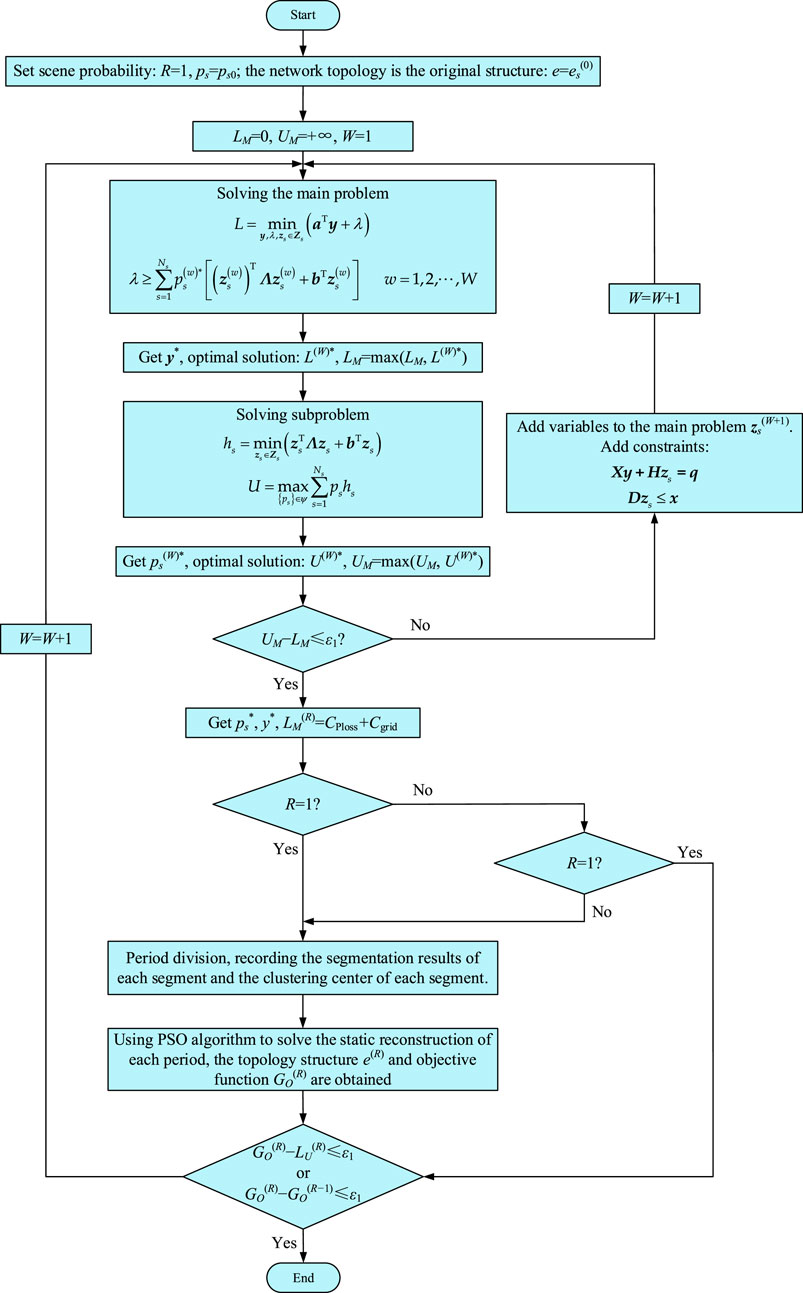
To sum up, the model can be solved by combining C&CG algorithm and particle swarm optimization algorithm, and its flow chart is shown in Figure 3.

Step 1: Set scenario probability R = 1, p_s = p_s0 in (Equation 60), and initialize the network topology e = e_s⁽⁰⁾ in (Equation 42);

Step 2: Set the upper limit L_M of the main problem model in (61), the lower limit U_M of the model in (Equation 65), and the initial value W = 1 for the number of iterations of the model;

Step 3: Solve the main problem model in (Equations 61, 62), and get the maximum value of variable y^* and model lower limit L_M;

Step 4: Then solve the sub-problem in (Equations 64–65), and get the minimum value of variable p_s^* and the upper limit U_M of the model;

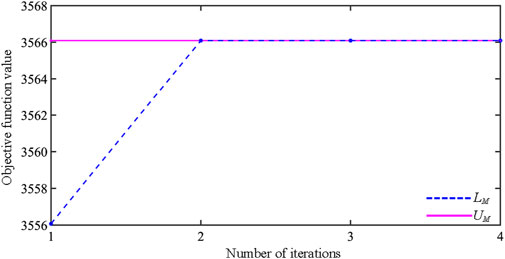
Step 5: Determine whether the difference between L_M and U_M is within the ideal range ε₁: if yes, variables p_s^* and y^* are obtained, and a joint solution L_U^(R) of network loss cost C_Ploss and main network power purchase cost C_grid is established; if the range of ε₁ is not satisfied, add variable z_s^(W+1) to the main problem model in (Equations 61, 62) and constraints in (Equation 52) and (Equation 54), and increase the number of iterations W to return to Step 3; (In Figure 4 below, the curves of the upper L_M and lower U_M values with the number of iterations in the actual simulation analysis are given);

Step 6: Then determine whether the actual number R of the scenario distribution is 1: if yes, the period is divided, and the segmentation results and clustering center of each segment are recorded; if the number of iterations R is not 1, it is judged whether the failure range of L_U^(R) before and after is within ε₁: if yes, the model solution is completed; if not, the period division process is directly carried out.

Step 7: After the clustering center of each segment is obtained, the PSO algorithm is used to solve the static reconstruction of each period, and the topology e^(R) and the objective function G_O^(R) are obtained;

Step 8: Further determine whether the error of G_O^(R) and L_U^(R) or the error of G_O^(R) before and after two times is within the ideal range ε₁: if yes, the model is solved; If no, increase the number of iterations and return to Step 3.

Figure 3

Figure 3. Flow chart of model solving.

Figure 4

Figure 4. Variation of boundary value of main problem model.

5 Example analysis

5.1 Example introduction

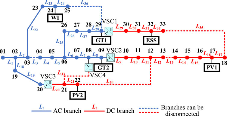
The efficacy of the model and algorithm presented in this treatise was validated utilizing the IEEE 33-node system (Ahmed and Salama, 2019), as depicted in Figure 5.

Figure 5

Figure 5. IEEE33-node AC-DC regional distribution network.

The IEEE 33-node system, characterized by a nominal voltage of 12.66 kV and a rated power capacity of 10 MW for each node, was configured with a particle swarm population size of 60 and subjected to 200 iterations. Relevant data pertaining to the wind turbines, PV power stations, reactive power compensation devices, and turbines are presented in Table 1, while the data concerning the ESS are detailed in Table 2. The network loss and the cost associated with curtailed wind and solar power were set at $50 per (MW·h) (Zhou et al., 2019). The cost of purchasing electricity from the main grid was referenced from (Wang et al., 2017). The aging cost per unit of charge-discharge energy for energy storage was determined to be $0.3 per (MW·h) (Shi et al., 2019). The start-up and operational costs for the GTs were derived from (Wang et al., 1995), with the specifics provided in Table 3.

Table 1

Table 1. Some parameters for IEEE33-node of DGs.

Table 2

Table 2. ESS parameters of IEEE33-node.

Table 3

Table 3. GT cost parameters of IEEE 33-node.

5.2 Model error analysis

Firstly, the prediction error of the two-phase RCO model proposed in this paper is investigated. And the following error indexes Δ_j,t ^diff are defined as Equation 67 as follows:

${\Delta }_{j,t}^{diff}=\left|P_{j,t}^2+Q_{j,t}^2-{\stackrel{\sim }{I}}_{ij,t}{\stackrel{\sim }{V}}_{i,t}\right|(67)$

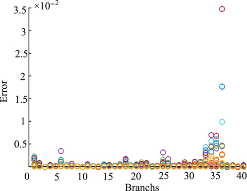
Aiming to maximize regional distribution network entity profits, the computation incorporated demand response and branch reconfiguration strategies. The error indices for all branches were calculated, with the error distribution illustrated in Figure 6. It is readily apparent that the error-index of the two-phase RCO model is at the magnitude of 10^–2, demonstrating a precision level that adequately meets the practical requirements of engineering applications.

Figure 6

Figure 6. Error scatter of all branches.

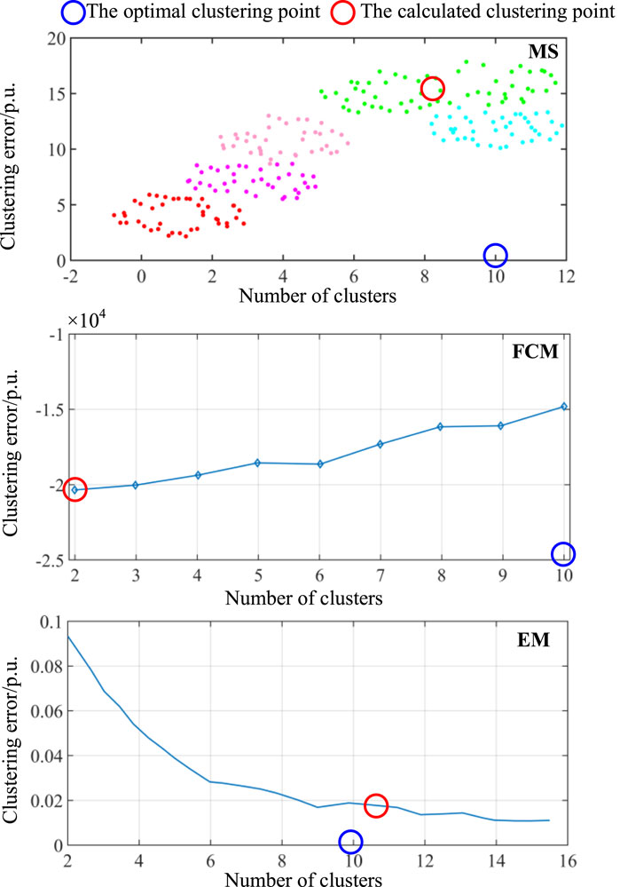
Then the clustering error of EM combined with K-means with in the two-phase RCO mode proposed in this paper. Here, the mean-shift (MS) algorithm (Wang et al., 2015), the fuzzy C-means (FCM) clustering algorithm (Kim et al., 2018), and the EM algorithm, were each combined with the fixed K-means algorithm for comparative analysis. 80 data points were randomly given for the clustering test, and the results are presented in Figure 7 and Table 4.

Figure 7

Figure 7. Comparison of clustering errors.

Table 4

Table 4. Clustering error of different algorithms.

The data obtained from the LHS was subjected to scenario clustering, and a comparative analysis was conducted among three algorithms to ascertain the optimal number of clusters. The results indicate that the number of clusters determined by the EM is most favorable. Application of the EM to verify the number of clusters for the IEEE 33-node system revealed a graphical representation of clustering error concerning the number of clusters, as depicted in Figure 7. It can be observed from Figure 7 that when the number of clusters is less than 10, the decline in clustering error is significant, whereas the rate of decrease markedly slows when the number of clusters exceeds 10. Adhering to the principles of the EM, the optimal number of clusters for the sample data is determined to be 10, which concurs with the referenced number of clusters. In contrast, the MS and FCM algorithms yielded cluster counts of 8 and 2 under the same sample data, deviating considerably from the referenced cluster count.

The sophisticated heuristic employed in this paper, which amalgamates the EM with K-means clustering, manifests a heightened precision in the computational aggregation of the sampled data points. As illustrated in Figure 8, an intricate analysis matrix, contingent upon the stochastic sampling data depicted in Figure 7, is orchestrating through the modification of load parameters, thereby yielding the comprehensive synthesis of period-scenario-power as proposed by the current model. This further attests to the efficacy of the two-phase RCO mode in processing integrated energy data, as well as its versatility in scenario generation.

Figure 8

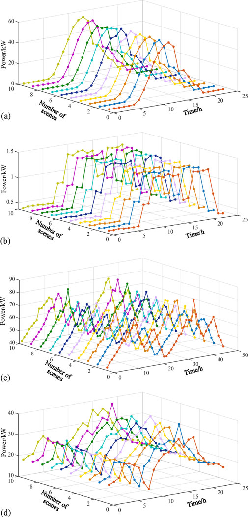
Figure 8. Time-scenario-power comprehensive analysis diagram: (A) Scenario analysis 1; (B) Scenario analysis 2; (C) Scenario analysis 3; (D) Scenario analysis 4.

The overall trend of energy in Figure 8A shows a flat peak between 8 h and 13h, reaching 1.3 kW, then decreasing to 0.7 kW between 15 h and 17 h, then rising to a flat peak after 18:00, and then decreasing at 21 h. The appearance of two energy peaks corresponds to the intensive activity time of people in the local distribution network. The longitudinal observation of the 10 scenarios shows that the EM-K-means has a strong precision error control performance.

In Figure 8B, the overall trend of energy fluctuates strongly, rising alternately at 8 h, 15 h, 30 h, 35 h and 42 h, and the peak energy continues to range from 70 kW to 80 kW. At this time, the robustness of EM-K-means can be reflected, and the energy difference between different scenarios is small, which proves that the proposed model forms a stable energy value in the initial optimization stage.

The energy optimization curve in Figure 8C has undergone a changing process of rising, falling, and rising again. The designed model fine-tuned the energy curve when considering the influencing factors of different scenarios, and it can be seen that the energy curve under different scenarios has a slight difference in peak point and bottom point, but the overall trend of change has maintained a good consistency. The superiority of EM-K-means method is proved.

The energy optimization curve in Figure 8D gradually rose after 5 h, reached a peak at 13 h, 55 kW, and then began to decline until the energy dropped to the lowest value after 18 h. In this process, with the change of the number of scenarios, the consistency of the energy curve is good, and the energy optimization at the peak point gradually flattens with the increase of the number of model iterations, and the optimal value is obtained.

5.3 Model robust optimization analysis and comparison

The deterministic model is compared with the two-phase RCO mode proposed in this paper. And the individual facility outputs and system network topology are determined under the premise of forecasted loads and renewable energy outputs. Subsequently, the resultant data are input into the ten scenarios obtained through clustering in Figure 8A, calculating the total system cost for each scenario. With the initial probability distribution as the starting point, optimization is conducted. The objective function is the sum of the cost probability distributions, yielding the facility outputs and scenario-specific costs as delineated in Table 5. An illustrative voltage curve for node 17 in Figure 5 under any given scenario is provided in Figure 9.

Table 5

Table 5. Cost comparison of different models in different scenarios.

Figure 9

Figure 9. Voltage of node 17 under the deterministic model.

It can be observed from Table 5 and Figure 9 that the two-phase RCO model proposed in this paper optimizes the system output across diverse scenarios, resulting in minimal network losses while ensuring safe operation under all conditions. This model adeptly adapts to the uncertainties within the system. Conversely, the optimization scheme derived from the deterministic model is susceptible to fluctuations in renewable energy and load, potentially leading to an increase in the total system cost and even causing node voltage to exceed limits, thus posing a threat to the system’s security and demonstrating inferior applicability.

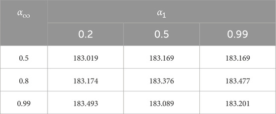
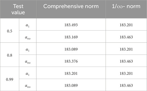
Given the scenario analysis-derived costs for each scenario as known conditions, RO is performed under the considerations of the comprehensive norm, solely the 1-norm, and solely the ∞-norm. The costs under these three scenarios are presented in Tables 6, 7, 8. When considering only the 1-norm, it is assumed that α₁ = 0.5, 0.5≤α_∞≤0.99. When considering only the ∞-norm, α_∞ is set at 0.99, with 0.2≤α₁ ≤ 0.99.

Table 6

Table 6. Comparison of total costs at different confidence levels.

Table 7

Table 7. Cost comparison of comprehensive norm and 1-norm and ∞-norm.

Table 8

Table 8. Solving time comparison.

The data presented in Table 6 reveal that as the values of α₁ and α_∞ increase, the confidence interval expands, encompassing a broader range of uncertainty probability distributions, which in turn leads to a higher total system cost. Additionally, when the value of α₁ is significant, the total system cost does not increase proportionally with the increase in α₁, indicating that the optimization outcome is predominantly influenced by the ∞-norm. As evidenced by Table 7, when optimization is performed considering only the 1-norm or solely the ∞-norm, the system adopts a more conservative approach, resulting in higher total costs.

5.4 Model solving speed analysis

To ascertain the computational speed performance of the two-phase RCO model proposed in this paper, the MS algorithm, the FCM clustering algorithm are also addressed here to be compared with the EM algorithm. The objective functions 1 to 4 are, respectively: minimizing network loss (OF1); minimizing electricity purchase from the main grid (OF2); minimizing the sum of network loss and electricity purchase from the main grid (OF3); and maximizing the main grid’s profit considering curtailed wind and solar power, the cost of GTs, and CO₂ emissions cost (OF4). And the results are presented in Table 8.

The data in Table 5 reveal that as the objective function’s scope expands, the EM model’s computational time increases accordingly. Nonetheless, the calculation speed remains acceptable, with the maximum solving time reaching 57.18 s. In comparison to the MS and FCM models, the EM model’s solving time is reduced by an average of 30.1% and 36.84%, respectively, thereby enhancing the efficiency of the solution process.

5.5 Scenario generation analysis

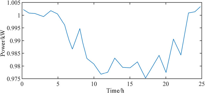
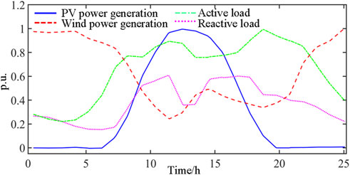
The forecasted output curves for the load, PV, and wind power devices are as depicted in Figure 10, wherein the time-series curves for all load nodes correspond to the curve shown in Figure 10. The predictive error conforms with a normal distribution, with a mean of zero and a variance equivalent to 21% of the predicted value.

Figure 10

Figure 10. Predicted power of wind turbine, PV and load.

The correlation coefficients between the forecasted outputs of the load, PV, and wind power devices, as well as among different PV and wind power devices, are presented in Table 9. In the table, the device numbers 1 and 2 denote PV generation, numbers 3 and 4 represent wind power generation, while numbers 5 and 6 correspond to the active and reactive loads of the system, respectively. For clarity of observation, the outputs of PV and wind power have been scaled down to 0.1, and the active and reactive loads to 0.001.

Table 9

Table 9. The correlation coefficient between each unit.

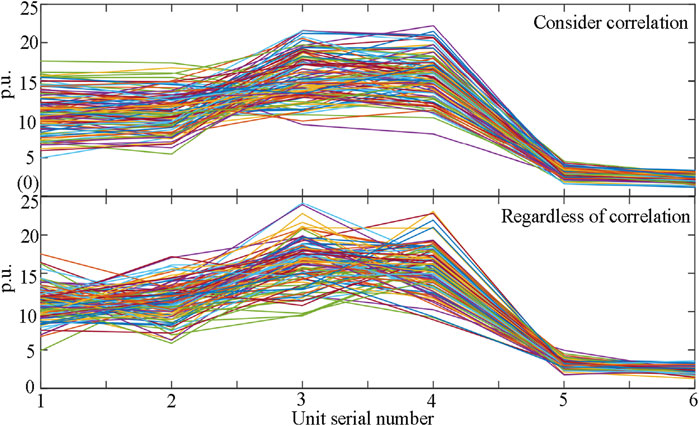
Utilizing LHS, a total of 80 scenarios with distinct correlations and 80 without correlations among the devices were generated, as illustrated in Figure 11. By comparing the correlation coefficient matrix, it is evident from Figure 11 that when considering correlations, the positive inter-device correlations result in approximately parallel lines; conversely, without considering correlations, the device outputs are unconstrained, leading to more chaotic and disordered lines.

Figure 11

Figure 11. Sampling scenario correlation analysis.

K-means clustering algorithm is used for scenario clustering. This paper selects four typical scenarios for comprehensive energy system optimization analysis, as shown in Figures 12–15.

Figure 12

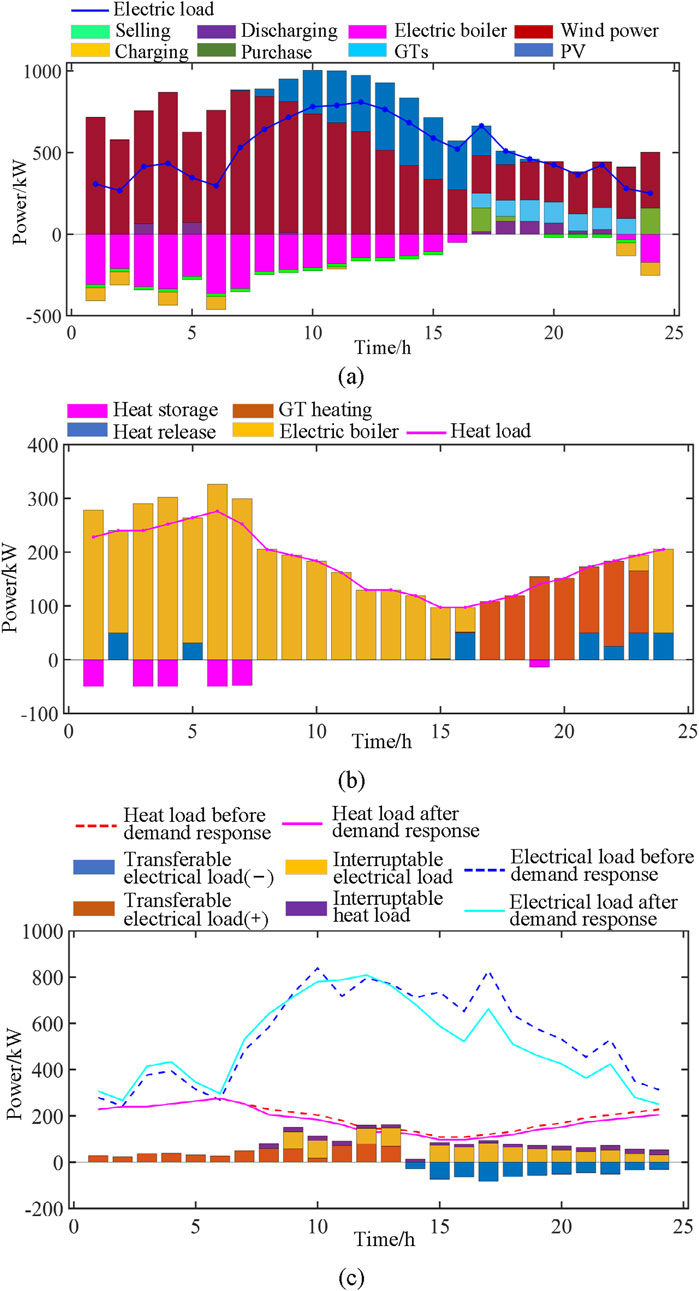
Figure 12. Scenario 1 comprehensive energy analysis results: (A) Electrical energy variation diagram; (B) Thermal energy variation diagram; (C) Electric-heat load response curve.

Figure 13

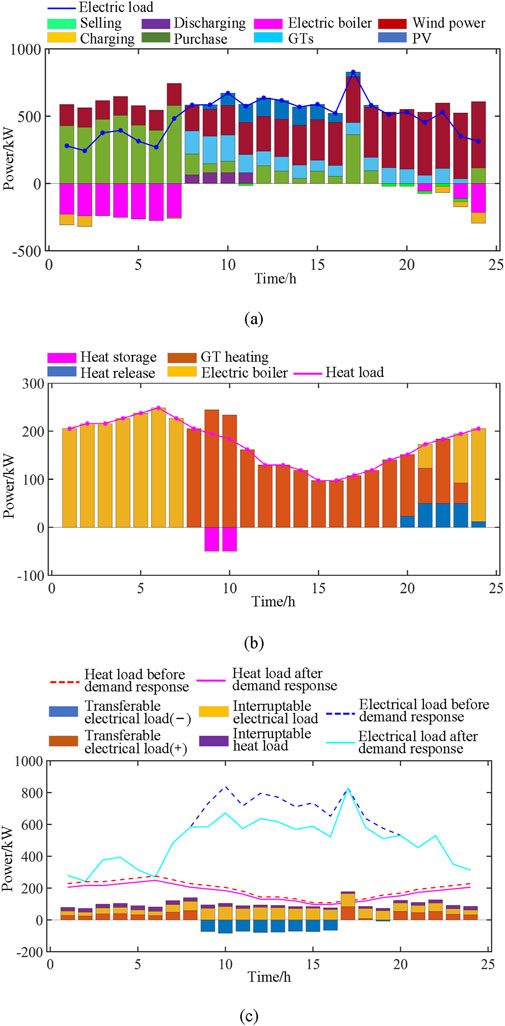
Figure 13. Scenario 2 comprehensive energy analysis results: (A) Electrical energy variation diagram; (B) Thermal energy variation diagram; (C) Electric-heat load response curve.

Figure 14

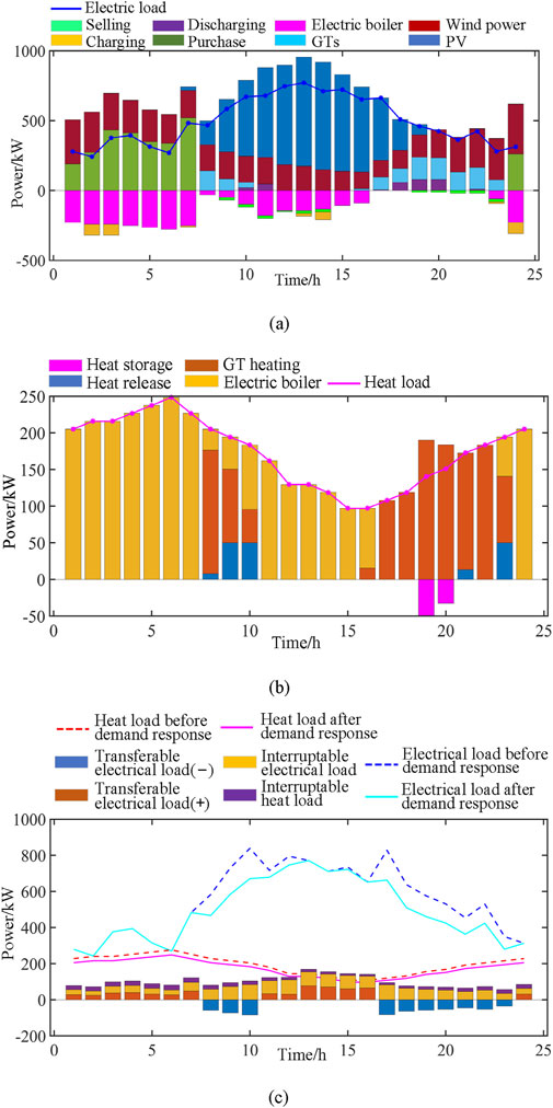
Figure 14. Scenario 3 comprehensive energy analysis results: (A) Electrical energy variation diagram; (B) Thermal energy variation diagram; (C) Electric-heat load response curve.

Figure 15

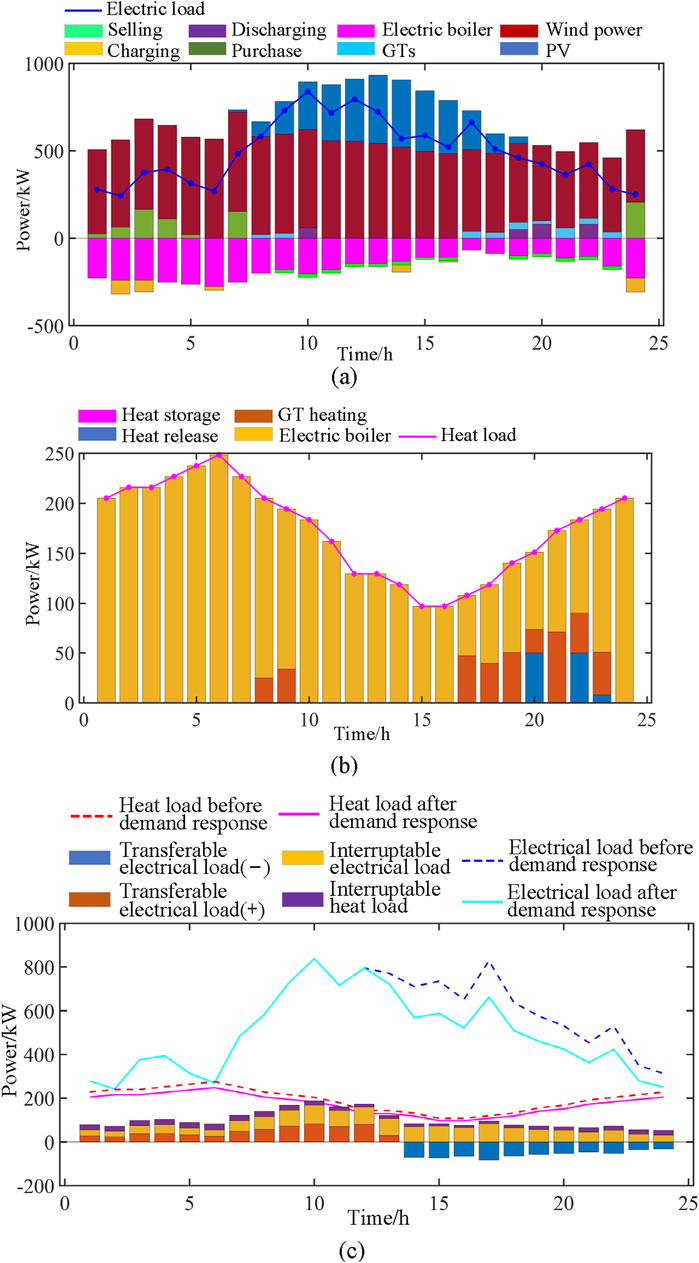
Figure 15. Scenario 4 comprehensive energy analysis results: (A) Electrical energy variation diagram; (B) Thermal energy variation diagram; (C) Electric-heat load response curve.

5.5.1 Scenarios 1

As shown in Figure 12A, from 0:00, wind power as the main power supply began to rise gradually, peaked at around 8:00, and then began to decline. In this period of time, the electric boiler is the main object of electricity, and this stage is also the rising moment of charging data. After 8:00, PV as an auxiliary energy source for power generation began to gradually rise at about 13:00 to reach a peak, and in the process, wind power was still stable. After reaching 15:00, due to the apparent decline in PV and wind power, the amount of electricity purchased began to rise briefly. At this time, the GT power generation begins to start, and phased power purchase behavior appears in this transition stage. In the whole scenario, the electric load peaks at around 10:00, peaks in phases when the GT generates power, and then begins to decline slowly.

In the thermal energy variation diagram of the scene in Figure 12B, corresponding to the changes in Figure 12A, the energy variation of the electric boiler shows an upward trend from 0:00 to 8:00, and the heat storage gradually accumulates in the process. After that, the heat energy of the electric boiler began to decline with the decline of wind power energy. At around 16:00, due to the start-up of GT power generation, GT heat supply gradually increases. In order to maintain the stability of heat energy, there is intermittent heat release from 15:00 to 24:00. The heat load of the whole process system reaches a branch at around 7:00, and then gradually declines until the GT starts at around 16:00, driving the heat load to rise again.

The influence curve of the point heat load in Figure 12C aligns with the trends observed in Figures 12B,C, reflecting the dynamic nature of energy consumption patterns. Our designed model adeptly captures and adjusts to these fluctuations, as evidenced by the overall increase in the demand response electrical load after 8:00, which peaks in two distinct stages around 10:00 and 16:00. In contrast, the thermal load displays an inverse pattern, showcasing the model’s capability to handle the divergent trends of electrical and thermal loads. This responsiveness is a direct outcome of the model’s RO strategy, which is tailored to manage and mitigate the impacts of data fluctuation, ensuring that energy distribution remains efficient and balanced even as consumption patterns evolve throughout the day.

5.5.2 Scenarios 2

As shown in Figure 13A, from 00:00 onwards, with the increase of wind power, the purchased electricity also increased significantly, and the electric boiler also began to work, and the charging amount also began to increase. Until 8:00, when PV occupies the main power generation, the use of electric boilers drops sharply, and GT power generation also starts at this time, resulting in a significant decline in purchased electricity. However, although wind power decreases at this stage, it still maintains a stable level of 400 kW. By 16:00, wind power, purchased power, PV power generation surge, and then PV power generation gradually decline, wind power stabilized near 600 kW, supporting the overall system power generation; After 20:00, the decrease in temperature leads to an upward trend in the use of electric boilers.

The heat load data presented in Figure 13B exhibits a distinct pattern throughout the day. The period from 0:00 to 8:00 shows an increasing trend in heat load, coinciding with a time of lower ambient temperatures. As depicted in Figure 13A, the noticeable surge in GT heating that begins around 9:00 aligns with the initiation of GT power generation, indicating a direct correlation between power production and heating requirements. By 16:00, the system heat load reaches its nadir before starting a gradual ascent. This dip and subsequent rise are characteristic of the system’s thermal response, with a significant heat release occurring in stages after 20:00, possibly due to the decreased demand for heating as the day progresses.

In Figure 13C, the point load response curve not only illustrates the peak electricity consumption occurring around 10:00 and 18:00, which corresponds to higher energy use during morning and evening activities, but it also showcases our model’s proficiency in managing data fluctuation. The model adeptly captures the variation in energy demand, as the heat load response peaks around 8:00, mirroring the start of the day when the demand for heat is highest. Subsequently, the model’s optimization strategies enable the heat load to decrease until it resumes an upward trend after 16:00, in synergy with the increased utilization of GT heating.

This pattern suggests that the designed model is not only effectively managing the thermal load but is also capable of anticipating and responding to the changing energy demands. The peak in heat load occurring before the peak in electricity consumption is a testament to the system’s ability to adapt to the temporal dependencies and fluctuations in energy use. The model’s robust design ensures that it can dynamically adjust to these shifts, maintaining optimal energy distribution and utilization across both electrical and thermal loads.

5.5.3 Scenarios 3

The characteristics of the scene shown in Figure 14A are similar to those in Figure 13A. From 0:00 to 8:00 in the initial stage, both wind power and purchased electricity show an upward trend. Due to the low temperature, the usage of electric heating furnace also increases significantly. However, the difference is that in this scenario, starting at 8:00, PV power generation starts to rise sharply, reaches a peak at around 13:00, and then begins to decline slowly until around 20:00, PV power generation is still maintained near 500 kW; The surge of PV power generation replaces the output of wind power, which is relatively low in this stage, and the two form a good complementary relationship. After 20:00, with the weakening of PV power generation, wind power gradually increased, and the process was accompanied by heat release; And the electric furnace is put into use after 23:00.

Compared with Figure 13B, the change of thermal energy shown in Figure 14B is significantly different from that shown in Figure 13B: GT heating starts to rise from 8:00, and although it shows a downward trend after 11:00, it still replaces electric boiler heating as the main body of thermal energy and remains there until 23:00.

The transferable electrical load (−) in Figure 14C exhibits a more evenly distributed demand pattern, with notable peaks from 8:00 to 11:00 and again from 16:00 to 24:00, as opposed to the more concentrated load observed in the earlier hours of Figure 13C. This change in load distribution reflects the diurnal rhythm of energy usage and the complementary role of renewable energy sources like wind and PV, as illustrated in Figure 14A. Our model adeptly captures these dynamics, adjusting to the ebb and flow of energy supply and demand, ensuring a balanced and responsive energy management approach that aligns with the natural fluctuations of renewable energy generation.

5.5.4 Scenarios 4

As can be seen from Figure 15A, the characteristics of scenario 4 are that wind power plays the leading role in the whole power generation process, and the electric boiler continues to work in the whole process. At about 6:00, the PV access and began to continue to generate electricity, and reached a peak at around 13:00, after which it began to slowly decline until 20:00. The purchased electricity only occurs from 0:00 to 6:00, and is less than 200 kW; GT power generation began to be put into use after 17:00; And from 9:00, the sale of electricity began to maintain around 200 kW, and continued until 23:00.

Figure 15B clearly illustrates the dominant role of the electric heating furnace in the overall heating demand, a trend directly influenced by the operational pattern of the furnace shown in Figure 15A. The prominence of the electric heating furnace suggests that it is a primary source of heat during the observed period. Additionally, the GT heating depicted in the same figure aligns with the gas turbine power supply periods from 8:00 to 10:00 and 16:00 to 24:00, indicating a coordinated effort to manage both heating and power generation. The intermittent heat release process that initiates after 20:00 is a notable feature, possibly reflecting a reduced demand for immediate heating or a strategic shift in energy management to balance the system.

In Figure 15C, the electrical load reaches its zenith around 10:00 and 17:00, which aligns with peak usage times such as morning routines and evening activities. Concurrently, the transferable electrical load (−) remains relatively stable at approximately 100 kW from 14:00 onwards, indicating a period of consistent energy transfer or a balanced state within the system. This stability is a testament to our model’s ability to effectively manage and mitigate data fluctuation, maintaining a steady energy flow even during periods of high demand.

The energy component processing and optimization analysis across the four typical scenarios further confirm the efficacy of the proposed two-phase RCO model. It not only handles the complexities of energy distribution but also showcases its robustness in conducting detailed energy composition analysis and planning optimal goals within varying scenarios. This demonstrates the model’s systematic and efficient approach to energy management, which is particularly critical in dealing with the fluctuations and uncertainties inherent in renewable energy integration and shifting load demands.

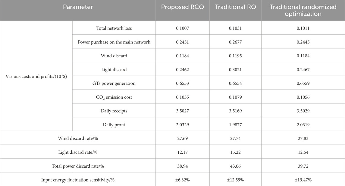
Based on the relevant data in the above four scenarios, the traditional randomized optimization (Liao et al., 2014) and traditional RO (Hosseini et al., 2014) method are introduced to compared with the two-phase RCO model. The results are shown in Table 10 below.

Table 10

Table 10. The correlation coefficient between each unit.

As can be seen from Table 10, the traditional RO planning corresponding to the clean energy consumption rate and the distribution network main profit is the smallest. The optimization results corresponding to stochastic programming have the best economy and clean energy consumption rate, but the conservatism cannot be guaranteed. Compared with RO and stochastic programming, the two-stage RCO method proposed in this paper can achieve a better balance between economy and conservatism, maximize the profit of distribution network, and improve the absorption rate of clean energy, which has more advantages in dealing with uncertain planning. And the proposed RCO significantly contributes to the field by advancing a robust optimization framework for regional distribution networks, enhancing the integration of renewable energy, and improving system reliability. Moreover, the two-stage RCO model has a strong sensitivity to input energy fluctuation, reaching ±6.32%, which is ±6.27% and ±13.15% higher than that of traditional RO and traditional randomized optimization respectively. These advancements offer substantial benefits to power utility companies and distribution system operators, including cost savings, efficiency gains, reduced energy curtailment, and support for grid modernization, ultimately bolstering their competitiveness and service quality.

6 Conclusion

In the wake of contemplating the unpredictability of wind, solar, and load generation outputs, this study has developed a RCO model anchored in energy storage, GTs, reactive power compensation devices, and network topological structures. Through the solution and analysis of the IEEE 33-node system, the following conclusions have been elucidated:

1) The scenario generation approach is pivotal in influencing the optimization outcomes. Utilizing LHS, which considers the correlation coefficient matrix, adeptly captures the interdependencies among various devices. An enhanced scenario clustering algorithm, capable of adaptively determining the number of clusters based on sample data, exhibits higher practicality, minimal clustering error, improved robustness, and superior representativeness of the scenarios.

2) Integrating energy storage and GTs into the system, or alterations to the network structure, augments the system’s flexibility and significantly enhances its operational economy.

3) The distributed robust optimization model, building upon the stochastic optimization framework, incorporates the confidence intervals of probability distributions, effectively balancing the economic considerations of the system.

In a future extension of our work, we indeed plan to incorporate optimal control strategies to enhance the dynamic management of distributed energy resources within the distribution network. Further making the lightweight design of the optimization model and aiming to enhance scenario generation and multi-objective optimization for comprehensive economic, environmental, and reliability analysis. The application of smart grids and the extension of optimization models to more complex energy systems will also be further considered.

Data availability statement

The original contributions presented in the study are included in the article/Supplementary Material, further inquiries can be directed to the corresponding authors.

Author contributions

HM: Writing–review and editing, Validation, Software, Resources, Project administration, Funding acquisition, Conceptualization. WZ: Writing–original draft, Validation, Software, Methodology, Formal Analysis, Data curation, Conceptualization. AW: Writing–original draft, Validation, Supervision, Investigation.

Funding

The author(s) declare that financial support was received for the research, authorship, and/or publication of this article. This research was funded by 2024 Special Fund for Science and Technology Innovation Strategy of Guangdong Province (Science and Technology Innovation Cultivation of College Students), grant number pdjh 2024a706.

Conflict of interest

The authors declare that the research was conducted in the absence of any commercial or financial relationships that could be construed as a potential conflict of interest.

Publisher’s note

All claims expressed in this article are solely those of the authors and do not necessarily represent those of their affiliated organizations, or those of the publisher, the editors and the reviewers. Any product that may be evaluated in this article, or claim that may be made by its manufacturer, is not guaranteed or endorsed by the publisher.

Supplementary material

The Supplementary Material for this article can be found online at: https://www.frontiersin.org/articles/10.3389/fenrg.2024.1496302/full#supplementary-material

References

Abboud, A., Iutzeler, F., Couillet, R., Debbah, M., and Siguerdidjane, H. (2016). Distributed production-sharing optimization and application to power grid networks. Signal Inf. Proc. Netw. 2, 16–28. doi:10.1109/tsipn.2015.2509182

CrossRef Full Text | Google Scholar

Ahmed, H. M. A., and Salama, M. M. A. (2019). Energy management of AC–DC hybrid distribution systems considering network reconfiguration. IEEE Trans. Power Syst. 34 (6), 4583–4594. doi:10.1109/tpwrs.2019.2916227

CrossRef Full Text | Google Scholar

Bagheri, A., Wang, J., and Zhao, C. (2017). Data-driven stochastic transmission expansion planning. IEEE Trans. Power Syst. 32, 3461–3470. doi:10.1109/tpwrs.2016.2635098

CrossRef Full Text | Google Scholar

Barni, M. (1997). A fast algorithm for 1-norm vector median filtering. IEEE Trans. Image Process 6, 1452–1455. doi:10.1109/83.624972

PubMed Abstract | CrossRef Full Text | Google Scholar

Bürger, M., Notarstefano, G., and Allgöwer, F. (2014). A polyhedral approximation framework for convex and robust distributed optimization. IEEE Trans. Autom. Control 59, 384–395. doi:10.1109/tac.2013.2281883

CrossRef Full Text | Google Scholar

Campo, P. J., and Morari, M. (1986). “∞-norm formulation of model predictive control problems,” in Proceedings of American control conference (Seattle, America), 18–20.

CrossRef Full Text | Google Scholar

Cheng, J., Wang, L., and Pan, T. (2023). Optimized configuration of distributed power generation based on multi-stakeholder and energy storage synergy. IEEE Access 11, 129773–129787. doi:10.1109/access.2023.3334008

CrossRef Full Text | Google Scholar

Darivianakis, G., Eichler, A., Smith, R. S., and Lygeros, J. (2017). A data-driven stochastic optimization approach to the seasonal storage energy management. IEEE Control Syst. Lett. 1, 394–399. doi:10.1109/lcsys.2017.2714426

CrossRef Full Text | Google Scholar

Hakkarinen, D., Wu, P., and Chen, Z. (2015). Fail-stop failure algorithm-based fault tolerance for Cholesky decomposition. IEEE Trans. Parallel Distrib. Syst. 26, 1323–1335. doi:10.1109/tpds.2014.2320502

CrossRef Full Text | Google Scholar

Hosseini, S., Farahani, R. Z., Dullaert, W., Raa, B., Rajabi, M., and Bolhari, A. (2014). A robust optimization model for a supply chain under uncertainty. IMA J. Manag. Math. 25 (4), 387–402. doi:10.1093/imaman/dpt014

CrossRef Full Text | Google Scholar

Hu, B., Li, Y., Yang, H., and Wang, H. (2017). Wind speed model based on kernel density estimation and its application in reliability assessment of generating systems. J. Mod. Power Syst. Clean. Energy 5, 220–227. doi:10.1007/s40565-015-0172-5

CrossRef Full Text | Google Scholar

Kim, E. H., Oh, S. K., and Pedrycz, W. (2018). Design of reinforced interval type-2 fuzzy C-Means-Based fuzzy classifier. IEEE Trans. Fuzzy Syst. 26, 3054–3068. doi:10.1109/tfuzz.2017.2785244

CrossRef Full Text | Google Scholar

Li, X., Wang, L., Yan, N., and Ma, R. (2021). Cooperative dispatch of distributed energy storage in distribution network with PV generation systems. IEEE Trans. Appl. Supercond. 31, 1–4. doi:10.1109/tasc.2021.3117750

CrossRef Full Text | Google Scholar

Liao, Y., Shen, J., Lin, Y., and Zhou, C. (2014). Quantitative analysis of network configuration in randomized distribution wireless sensor networks. IEEE Sens. J. 14 (6), 1974–1979. doi:10.1109/JSEN.2014.2306685

CrossRef Full Text | Google Scholar

Liu, F., and Deng, Y. (2021). Determine the number of unknown targets in open world based on elbow method. IEEE Trans. Fuzzy Syst. 29, 986–995. doi:10.1109/tfuzz.2020.2966182

CrossRef Full Text | Google Scholar

Mahdavi, M., Schmitt, L. E. K., and Jurado, F. (2023). Robust distribution network reconfiguration in the presence of distributed generation under uncertainty in demand and load variations. IEEE Trans. Power Deliv. 38, 3480–3495. doi:10.1109/tpwrd.2023.3277816

CrossRef Full Text | Google Scholar

Margellos, K., Goulart, P., and Lygeros, J. (2014). On the road between robust optimization and the scenario approach for chance constrained optimization problems. IEEE Trans. Autom. Control 59, 2258–2263. doi:10.1109/tac.2014.2303232

CrossRef Full Text | Google Scholar

Moghadam, M. R. V., Zhang, R., and Ma, R. T. B. (2016). Distributed frequency control via randomized response of electric vehicles in power grid. IEEE Trans. Sustain. Energy 7, 312–324. doi:10.1109/tste.2015.2494504

CrossRef Full Text | Google Scholar

Ratschan, S. (2002). Search heuristics for box decomposition methods. J. Glob. Optim. 24, 35–49. doi:10.1023/a:1016246616462

CrossRef Full Text | Google Scholar

Saaklayen, M. A., Liang, X., Faried, S. O., Martirano, L., and Sutherland, P. E. (2024). Soft open point-based service restoration coordinated with distributed generation in distribution networks. IEEE Trans. Ind. Appl. 60, 2554–2566. doi:10.1109/tia.2023.3332584

CrossRef Full Text | Google Scholar

Schouhamer Immink, K. A., and Weber, J. H. (2015). Hybrid minimum pearson and euclidean distance detection. IEEE Trans. Commun. 63, 3290–3298. doi:10.1109/tcomm.2015.2458319

CrossRef Full Text | Google Scholar

Shi, Y., Wang, L., Chen, W., and Guo, C. (2019). Distributed robust unit commitment with energy storage based on forecasting error clustering of wind power. Automation Electr. Power Syst. 43, 3–16.

Google Scholar

Shin, P. S., Woo, S. H., and Koh, C. S. (2009). An optimal design of large scale permanent magnet Pole shape using adaptive response surface method with Latin hypercube sampling strategy. IEEE Trans. Magn. 45, 1214–1217. doi:10.1109/tmag.2009.2012565

CrossRef Full Text | Google Scholar

Sinaga, K. P., and Yang, M. S. (2020). Unsupervised K-means clustering algorithm. IEEE Access 8, 80716–80727. doi:10.1109/access.2020.2988796

CrossRef Full Text | Google Scholar

Wada, T., and Fujisaki, Y. (2015). Sequential randomized algorithms for robust convex optimization. IEEE Trans. Autom. Control 60, 3356–3361. doi:10.1109/tac.2015.2423871

CrossRef Full Text | Google Scholar

Wang, B., Zhang, C., Li, C., Yang, G., and Dong, Z. Y. (2022). Transactive energy sharing in a microgrid via an enhanced distributed adaptive robust optimization approach. IEEE Trans. Smart Grid. 13, 2279–2293. doi:10.1109/tsg.2022.3152221

CrossRef Full Text | Google Scholar

Wang, C., Lei, S., Ju, P., Chen, C., Peng, C., and Hou, Y. (2020). MDP-based distribution network reconfiguration with renewable distributed generation: approximate dynamic programming approach. IEEE Trans. Smart Grid. 11, 3620–3631. doi:10.1109/tsg.2019.2963696

CrossRef Full Text | Google Scholar

Wang, L., Tang, D., Guo, Y., and Do, M. N. (2015). Common visual pattern discovery via nonlinear mean shift clustering. IEEE Trans. Image Process 24, 5442–5454. doi:10.1109/tip.2015.2481701

PubMed Abstract | CrossRef Full Text | Google Scholar

Wang, S., Chen, S., Ge, L., and Wu, L. (2016). Distributed generation hosting capacity evaluation for distribution systems considering the robust optimal operation of OLTC and SVC. IEEE Trans. Sustain. Energy 7, 1111–1123. doi:10.1109/tste.2016.2529627

CrossRef Full Text | Google Scholar

Wang, S., Chen, S., and Xie, S. (2017). Security-constrained coordinated economic dispatch of energy storage systems and converter stations for AC/DC distribution networks. Automation Electr. Power Syst. 41, 85–91.

Google Scholar

Wang, S. J., Shahidehpour, S. M., Kirschen, D. S., Mokhtari, S., and Irisarri, G. D. (1995). Short-term generation scheduling with transmission and environmental constraints using an augmented Lagrangian relaxation. IEEE Trans. Power Syst. 10, 1294–1301. doi:10.1109/59.466524

CrossRef Full Text | Google Scholar

Wang, X., Yang, W., and Liang, D. (2021). Multi-objective robust optimization of hybrid AC/DC distribution networks considering flexible interconnection devices. IEEE Access 9, 166048–166057. doi:10.1109/access.2021.3135609

CrossRef Full Text | Google Scholar

Yuan, W., Wang, J., Qiu, F., Chen, C., Kang, C., and Zeng, B. (2016). Robust optimization-based resilient distribution network planning against natural disasters. IEEE Trans. Smart Grid 7, 2817–2826. doi:10.1109/tsg.2015.2513048

CrossRef Full Text | Google Scholar

Zhang, C., Xu, Y., and Dong, Z. Y. (2018). Probability-weighted robust optimization for distributed generation planning in microgrids. IEEE Trans. Power Syst. 33, 7042–7051. doi:10.1109/tpwrs.2018.2849384

CrossRef Full Text | Google Scholar

Zhang, Y., Wang, J., and Li, Z. (2020). Interval state estimation with uncertainty of distributed generation and line parameters in unbalanced distribution systems. IEEE Trans. Power Syst. 35, 762–772. doi:10.1109/tpwrs.2019.2926445

CrossRef Full Text | Google Scholar

Zhang, Z., Wang, C., Lv, H., Liu, F., Sheng, H., and Yang, M. (2021). Day-ahead optimal dispatch for integrated energy system considering power-to-gas and dynamic pipeline networks. IEEE Trans. Ind. Appl. 57, 3317–3328. doi:10.1109/tia.2021.3076020

CrossRef Full Text | Google Scholar

Zhou, J., Hu, T., Liao, L., Gao, H., Hu, J., Wang, H., et al. (2019). “Economical operation optimization of distribution network considering multiple adjustment measures,” in Proceedings of IEEE PES innovative smart grid technologies asia, chengdue, China.

CrossRef Full Text | Google Scholar