Two-stage transient stability assessment using ensemble learning and cost sensitivity

This paper proposes a novel two-stage transient stability assessment (TSA) model that integrates ensemble learning with cost sensitivity to address the challenges posed by the integration of renewable energy and load fluctuations. The model employs CNNs as positive and negative classifiers to initially evaluate samples, with consistent results output directly. In cases of inconsistency, the sample is evaluated by a fair classifier, specifically an ELM, trained on critical samples. This approach significantly enhances the classification performance and credibility of the fair classifier, especially under imbalanced conditions, thereby improving the overall efficiency and accuracy of TSA. The proposed model demonstrates superior performance compared to single-stage models and other two-stage models, achieving high accuracy and robustness in transient stability assessment, particularly for critical samples.

1 Introduction

The development of modern power systems presents new challenges to the safety of these systems. In recent years, frequent blackouts worldwide have had significant economic impacts (Wei Zhang and Zhang, 202). Transient stability is crucial to the safe operation of power systems. Once a disturbance occurs in the power system, early assessment of transient stability and timely implementation of emergency control measures can protect the system’s stability (Guo et al., 2023; Meridji et al., 2023; Singh and Chauhan, 2023; Wang Y. et al., 2023; Zhu et al., 2023). Therefore, it is vital and necessary to design a TSA model that can quickly and accurately determine whether a power system will become unstable and infer the type of events that may cause instability.

Classical transient stability methods include time-domain simulation (TDS) and direct methods. TDS analyzes system stability through detailed modeling. As long as the component models and network structures are sufficiently accurate, the results are reliable. However, with the increasing complexity of power systems and rapid changes in electronic hardware, TDS-based models have become more complex, and their computational demands have increased, making TDS methods unsuitable for real-time transient stability assessment. The direct method, on the other hand, does not require numerical integration of dynamic processes and can quantitatively analyze system transient stability. However, direct method models are simple and may face applicability issues in complex power systems. Additionally, the evaluation results tend to be conservative. As a result, these methods currently cannot fully meet the practical needs of online transient stability assessment. To date, real-world power grids still require more advanced TSA solutions that can achieve high reliability and efficiency.

The rapid development of big data offers new ideas for transient stability assessment. TSA rules can be mined from large volumes of data using machine learning (ML) methods (Liu et al., 2023; Li et al., 2024; Shao et al., 2024). Once dynamic information is received, stability results can be output within milliseconds. After discovering underlying relationships offline through ML, they can be easily applied to online TSA. This data-driven approach almost eliminates online computation time and can effectively predict system stability.

Modern power systems usually remain stable after most disturbances due to their robustness. In practical applications, events causing power system instability are rare. These rare events lead to significant imbalances between stable (majority class) and unstable (minority class) transient data distributions. The imbalance in training data leads to high misclassification rates in TSA models. Moreover, misjudging the transient stability of power systems prevents timely responses and corresponding measures, leading to safety accidents and significant economic losses. Therefore, addressing the imbalance in training data is not only crucial for improving TSA accuracy but also has practical significance.

Existing methods for addressing class imbalance can be broadly categorized into data-driven and algorithm-driven approaches. Additionally, traditional data-driven methods attempt to oversample or undersample the data so that different classes appear in equal proportions in the training data. The main drawback of sampling-based methods is that they may lose important information in undersampling or overfit the training data in oversampling. Algorithm-driven methods primarily include cost-sensitive methods (Wang H. et al., 2023; Chen et al., 2022; Lin et al., 2022; Wang et al., 2020) and ensemble learning methods (Shen, 2023; Chen and Wang, 2021; Chen et al., 2021; Zhao et al., 2022; Wu et al., 2020). References (Wang H. et al., 2023) consider the imbalance in sample distribution in space by dividing samples into different levels of training sets and training the model using cost-sensitive approaches. Reference (Shen, 2023) proposes a comprehensive transient stability state assessment method for power systems based on machine learning, using multiple classifiers to alleviate the sample imbalance problem in transient stability samples. However, its drawbacks are also evident. The ensemble learning classifiers used are often weak classifiers with low resistance to interference and increased training time. Among these methods, the application of cost sensitivity in transient stability assessment is relatively limited. Although it helps mitigate sample imbalance, its blind use may lead to overfitting and increased misclassification rates. Applying ensemble learning alone to transient stability assessment can also mitigate sample imbalance, but due to the large number of ensemble classifiers, it may result in longer training times and weaker resistance to interference.

Recently, to mitigate the imbalance in transient stability samples, references (Chen and Wang, 2021; Wang et al., 2020) adopted a two-stage assessment approach combining cost sensitivity and ensemble learning. Specifically, three models are used, with two classifiers in the first stage, each biased towards one class of samples using cost-sensitive methods. A non-cost-sensitive classifier is then trained using the same training set as a fair classifier for second-stage evaluation. Although this approach combines the advantages of cost-sensitive learning and ensemble learning, it also overcomes some disadvantages. However, this method lacks credibility, mainly because the credibility of the fair classifier is low. This is because hard samples are evaluated by a non-cost-sensitive classifier, and the evaluation results are directly output. However, since the fair classifier is not selected based on the characteristics of the input samples, highly accurate and convincing evaluation results cannot be generated.

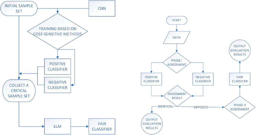
In transient stability assessment, what truly affects misclassification and missed judgments are the hard samples. In this study, we propose a two-stage transient stability assessment model based on the integration of ensemble learning and cost sensitivity. First, the initial sample set is input into positive and negative classifiers again, and samples with inconsistent evaluation results are collected to form a critical sample set. This critical sample set is used to train the ELM (fair classifier). The model combines the strengths of cost sensitivity and ensemble learning, greatly enhancing the credibility of the fair classifier while improving the overall reliability of the model.

The rest of this paper is structured as follows: Section 2 offers an overview of the transient stability assessment (TSA) problem and introduces the proposed two-stage TSA model. Section 3 details the implementation process of the model. Section 4 presents case studies and evaluates the model’s performance. Finally, Section 5 summarizes the conclusions of the paper.

2 Integrated TSA model

2.1 Transient stability assessment problem

Transient stability assessment (TSA) has become increasingly important in power systems, with the main challenge being how to overcome the inherent sample imbalance problem, which is determined by the robustness of power systems. To address the imbalance in transient stability samples, a two-stage assessment method combining cost sensitivity and ensemble learning has been widely adopted. However, due to the lack of optimization in the selection of the fair classifier, it is difficult to produce highly accurate and convincing evaluation results. The model proposed in this paper addresses the problem of transient stability assessment under imbalanced samples by considering the difficulty of classifying critical samples, combining cost sensitivity and ensemble learning, which greatly enhances the reliability of the fair classifier and the overall model reliability. Currently, the issue of sample imbalance in transient stability assessment cannot be ignored, as stable samples are the majority, unstable samples are fewer, and critical samples are even rarer. The training model must fully understand the characteristics of stable, unstable, and critical samples to classify them correctly. Therefore, solving the sample imbalance problem is crucial for transient stability assessment. The two-stage TSA model proposed in this paper aims to achieve accurate and reliable classification results even under imbalanced conditions.

2.2 Selection of positive and negative models and application of cost sensitivity

2.2.1 Selection of positive and negative models

Unlike most previous evaluation model designs, this paper designs a two-stage transient stability assessment model based on the integration of ensemble learning and cost sensitivity. The advantage of this approach is that it can combine the strengths of various models and effectively overcome the drawbacks of low accuracy, low effectiveness, and high cost caused by sample imbalance.

The positive and negative models are the foundational models in the entire two-stage framework; their results are only valid when they are consistent. Otherwise, if the results are inconsistent, the assessment will enter the next stage without directly outputting the results. Therefore, to maximize the role of the positive and negative models, cost sensitivity is applied to these models. The positive model is inclined to evaluate samples as stable, while the negative model is inclined to evaluate samples as unstable. Under this design, when the evaluation results of the positive and negative models are consistent, the input samples must be far from the boundary, indicating that the samples are either extremely stable or extremely unstable. In such cases, the positive and negative models require strong feature extraction capabilities to fully recognize samples beyond the boundary.

Convolutional Neural Networks (CNNs) possess strong nonlinear expression and pattern recognition capabilities, making them suitable for handling complex dynamic processes and nonlinear problems in power systems (Lee et al., 2023). This allows CNN-based TSA models to more accurately reflect the transient stability status of the power system based on input operational parameters. Compared to traditional time-domain and direct methods, CNN-based TSA methods offer higher assessment accuracy and faster computation speed. They can meet the requirements of online real-time prediction, providing timely and accurate power system stability analysis results for dispatchers (Gu et al., 2024). Additionally, CNN models can adapt to different power system scenarios and demands by adjusting the network structure and parameters, offering higher flexibility and scalability. In summary, applying CNNs to power system transient stability assessment has advantages such as automatic feature extraction, strong nonlinear processing capabilities, high accuracy, real-time performance, and applicability to complex systems, making it a vital tool in power system operation and control. Therefore, we select CNN as the positive and negative models. With CNN’s strong feature extraction capabilities, we can effectively handle the characteristics of stable and unstable sample regions, achieving initial simple classification. Furthermore, CNN-based methods can directly use low-level measurement data as input features, extracting multi-granularity information from measurement data through multi-size convolution kernels, thereby improving the accuracy of TSA in power systems (Jin et al., 2023).

For transient stability assessment, reasonable feature selection is needed to construct samples as input. This paper focuses on selecting steady-state quantities and fault characteristics for the forward-looking prediction of transient stability (Ji et al., 2022). Therefore, bus voltage, generator active and reactive power, and load active and reactive power are chosen as input features. Relevant data are obtained from measurements or time-domain simulations and input into the CNN model. The network structure of CNN is shown in Figure 1.

Figure 1

Figure 1. CNN network structure.

Based on the input electrical quantity matrix, the convolutional layer performs local learning through convolution kernels in the CNN model. The convolution operation for each convolution kernel is as Equation 1.

$a_{c,k}=f\left(X*W_{c,k}+b_{c,k}\right)(1)$

where $a_{c,k}$ is the output of the $k$-th convolutional surface, $W_{c,k}$ is the weight matrix corresponding to the $k$-th convolution kernel, $X$ is the input matrix, $b_{c,k}$ is the bias term, and $f(\cdot )$ is the activation function (the ReLU function is selected here).

For the pooling layer, this paper adopts max pooling, as shown in Equation 2.

$a_{p,k}=\max \left(a_{ij}\right),i,j=\mathrm{1,2},\dots ,n(2)$

where $a_{p,k}$ represents the $k$-th pooling surface, $a_{ij}$ is a sub-block of the output matrix from the previous convolutional layer, and $n$ is the dimension of the sub-block of the output matrix from the previous convolutional layer.

The calculation formula for the fully connected layer is as Equation 3.

$a_{fc}=f\left(a_p{W}_{fc}+b_{fc}\right)(3)$

In the fully connected layer, $a_{fc}$ represents the output, $a_p$ represents the input, $W_{fc}$ represents the weight matrix, and $b_{fc}$ represents the bias term. The ReLU function is selected for the activation function.

The fully connected layer passes the output values to the output layer, and the expression of the sigmoid function in the output layer is as Equation 4.

$\sigma \left(x\right)=\frac{1}{1+e^{-x}}(4)$

where $x$ is the input value and $\sigma (x)$ is the function output.

2.2.2 Application of cost sensitivity

Typically, the approach to solving quantity imbalance is to assign higher weights to unstable samples. However, the misclassification of critical samples still occurs. Another approach is to assign higher weights to both imbalances simultaneously: first, higher weights are given to unstable samples, and then higher weights are assigned to misclassified samples. This approach can lead to overfitting (Kesici et al., 2023).

In this study, the model is trained by optimizing parameters to improve the fit to the training samples. The loss function is used to measure the difference between the predicted and actual values, and the impact of training samples on evaluation rules can be assessed through the loss function. This cost-sensitive approach makes the positive model inclined to evaluate samples as stable and the negative model inclined to evaluate samples as unstable.

For the transient stability assessment problem, the weight correction coefficient for model parameters can be represented by Table 1.

Table 1

Table 1. Weight coefficient matrix for model parameter modification.

Where $C(\mathrm{1,1})=C(\mathrm{0,0})=0$. $C(\mathrm{1,0})$ and $C(\mathrm{0,1})$ represent the weight correction coefficients for model parameters when predicting stable conditions as unstable and unstable conditions as stable, respectively. Typically, $C(\mathrm{1,0})=C(\mathrm{0,1})=1$.

In different scenarios, the proportion of unstable samples to stable samples in the training set often differs, which causes the model trained under imbalanced samples to have a certain bias in its discriminative results. Therefore, this paper introduces a correction factor $\gamma$ to adjust for the imbalance in sample numbers in different scenarios, as shown in Equations 5, 6.

$\gamma \left(\mathrm{0,1}\right)=10(5)$

$\gamma \left(\mathrm{1,0}\right)=\frac{N_s}{N_{\mathit{uns}}}(6)$

where $N_s$ is the number of stable samples in the training set; $N_{\mathit{uns}}$ is the number of unstable samples in the training set.

By adjusting the weight correction coefficients during the evaluation model parameter correction process, the model’s loss function is as follows:

$Gp=-y^{\left(l\right)}\ln y^{\prime \left(l\right)}\gamma \left(\mathrm{1,0}\right)-\left[1-y^{\left(l\right)}\right]\ln \left[1-y^{\left(l\right)}\right]\gamma \left(\mathrm{0,1}\right)(7)$

The model using Equation 7 is the positive model. After applying cost sensitivity, this model tends to evaluate input samples as stable. Conversely, if the model needs to incline toward evaluating input samples as unstable, an additional correction factor $\beta$ is required. Since the original model tends to evaluate samples as stable due to sample imbalance, adding the coefficient $\beta$ ensures that the model tends to evaluate input samples as unstable. Similarly, it is also necessary to adjust the imbalance of the number of samples in different scenarios here, as shown in Equations 8, 9.

$\theta \left(\mathrm{0,1}\right)=\frac{N_s}{N_{\mathit{uns}}}(8)$

$\theta \left(\mathrm{1,0}\right)=10(9)$

When $\beta =1$, the evaluation model merely corrects for the bias introduced by the imbalanced training samples; when $\beta >1$, the model increases its fit to unstable samples, reducing the misclassification probability for unstable samples.

The reorganized model’s loss function is shown in Equation 10.

$Gn=-y^{\left(l\right)}\ln y^{\prime \left(l\right)}\theta \left(\mathrm{1,0}\right)-\beta \left[1-y^{\left(l\right)}\right]\ln \left[1-y^{\left(l\right)}\right]\theta \left(\mathrm{0,1}\right)(10)$

The negative model applies the loss function from the above equation to tend toward evaluating input samples as unstable.

2.3 Fair classifier

The fair classifier is used to classify hard samples, which are samples that the initial simple classification could not correctly categorize. Therefore, the sample set used to train the fair classifier is the critical sample set, and the model selection must consider this.

The fair classifier operates in the second stage of the assessment, requiring high accuracy and interpretability in its results. The sample set used to train the fair classifier is the critical sample set, which contains rich data information and high information entropy, requiring a suitable model to extract these features. For ELM training, the ideal sample should be data close to the stability boundary to obtain refined stability rules, allowing for effective learning of the critical region and a strong ability to correctly classify hard samples.

Given the above considerations, ELM is chosen as the fair classifier. Due to the distribution characteristics of the critical sample set, it matches the training requirements of the ELM model. If the training samples of ELM are from the critical region, the trained ELM will have a strong ability to correctly classify the critical sample set. ELM is used for training, but not with the original sample set; instead, it is trained using samples with conflicting evaluation results from two classifiers with opposing biases.

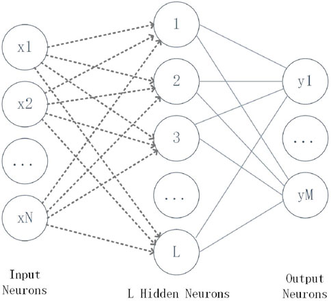
ELM can randomly select input layer parameters, and then use the Moore-Penrose generalized inverse to obtain the output layer weights with the smallest 2-norm. In ELM, only the number of hidden layer neuron nodes needs to be learned and adjusted, and the entire process does not require iteration. Figure 2 shows the ELM network structure.

Figure 2

Figure 2. Elm network structure.

Specifically, for a dataset $(x_i,y_i)$ with $N$ samples, where $x_i\in {\mathbb{R}}^n$ and $y_i\in {\mathbb{R}}^2$, $y_i$ is the class label of the $i$-th sample, and the ELM output with $M$ hidden layer units is shown in Equation 11.

$f\left(x_j\right)={\displaystyle \sum _{i=1}^m}{\beta }_{i}h\left(w_i{x}_j+b_i\right)=y_j(11)$

where $j=\mathrm{1,2},\dots ,N$; $h$ is the activation function; $w_i\in {\mathbb{R}}^n$ is the weight vector of the $i$-th unit in the hidden layer; ${\beta }_i\in {\mathbb{R}}^2$ is the multiplier of the $i$-th unit in the hidden layer; and $b_i\in {\mathbb{R}}^1$ is the bias of the $i$-th unit in the hidden layer.

In ELM, the weight vector $w_i$ and the bias $b_i$ are randomly assigned, and the multiplier ${\beta }_i$ can be obtained based on all the data through the Moore-Penrose generalized inverse. Therefore, there is no need for the backpropagation (BP) neural network’s necessary back-adjustment process (Fuqiang et al., 2023), making ELM’s calculation speed significantly faster than classification algorithms based on optimization. This reduction in calculation time also reduces the online application time of the two-stage evaluation model (Zhang et al., 2017).

2.4 Overall evaluation process

After completing all the above designs, the framework for the proposed two-stage transient stability assessment model is established. Next, the overall evaluation process is designed.

The model proposed in this study is a two-stage evaluation model, where the second stage’s evaluation somewhat depends on the results of the first stage. Therefore, it is necessary to design scoring for the first-stage evaluation results to complete the evaluation logic of the first and second stages.

Define $\lambda$, ${\lambda }_1$, ${\lambda }_2$, where $\lambda$ is the total score of the first stage, and ${\lambda }_1$, ${\lambda }_2$ are the scores of the positive and negative classifiers, respectively.

To improve efficiency, ${\lambda }_1$, ${\lambda }_2$ are linked to the output results of the positive and negative classifiers. If the positive classifier output is stable (label 1), then ${\lambda }_1$ is 1; otherwise, it is 0.

Define $\lambda ={\lambda }_1+{\lambda }_2$, the scoring logic is summarized in Table 2.

Table 2

Table 2. Scoring table.

According to the model logic proposed in this paper, the first-stage evaluation results are credible, and the evaluation results are directly output only when the positive and negative classifier outputs are consistent. This occurs when $\lambda$ is 0 or 2, meaning the first-stage evaluation results are reliable, and there is no need for the second-stage evaluation. If the positive and negative classifier outputs are inconsistent, the first-stage evaluation results are unreliable, and $\lambda$ equals 1, then the process proceeds to the second-stage evaluation.

The overall evaluation process can be simplified as shown in Table 3.

Table 3

Table 3. Evaluation process.

As shown in Table 3, when the total score is 1, the second-stage evaluation result is output as the model’s evaluation result. When the total score is 2, that is, when $\lambda$ equals 1, the first-stage evaluation result is credible, and the first-stage evaluation result is output as the model’s evaluation result.

3 Implementation process of the integrated TSA model

After selecting a specific example system, transient stability simulations are performed to collect steady-state data and create the initial sample set.

Based on the obtained initial dataset, the positive and negative classifiers are trained separately. After training, the initial dataset is re-input into the trained positive and negative classifiers for evaluation, and the critical dataset is organized based on the differing evaluation results from the positive and negative classifiers.

Since the fair classifier needs to correctly classify critical samples, ELM is selected as the fair classifier. By training ELM using the critical sample set, the ability of ELM to correctly classify critical samples is greatly enhanced, meeting the requirements of the fair classifier. The construction of the integrated TSA model is then completed.

When evaluating real-time data obtained from the power system, the measured data is input into the positive and negative classifiers for evaluation. If the evaluation results are consistent, the results are output, completing the assessment; if the evaluation results are inconsistent, the measured data is input into the fair classifier, and the evaluation results from the fair classifier are output, completing the assessment. The specific implementation process is shown in Figure 3.

(1): Offline Training

(2): Online Application

Figure 3

Figure 3. (1) Offline training; (2) Online application.

4 Case analysis

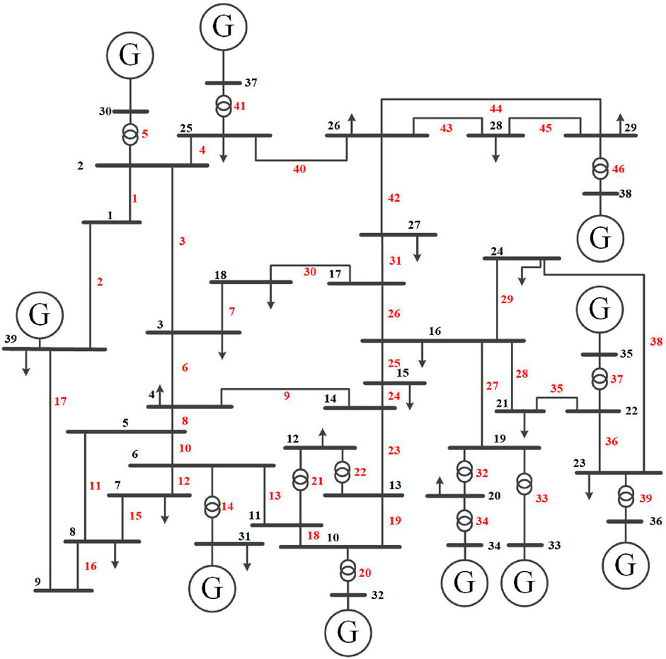
Taking the New England 10-generator, 39-bus system as a case study, as shown in the Figure 4, the entire bus system is divided into four regions according to adjacent buses. Four different load levels, 80%, 90%, 110%, and 120%, are considered, and each region is assigned a different load level, resulting in 256 different power flows,256 different operating modes. The generator output is adjusted accordingly to ensure the convergence of power flow calculations. The fault is set as a three-phase short-circuit fault, and an N-1 scan is performed on the system by sequentially setting faults on different lines. The fault duration is set to 0.2 s on lines without transformers, with the fault point located at 50% of the line’s length. On lines with transformers, the fault point is set at the head section of the line.

Figure 4

Figure 4. Line diagram of IEEE 39-bus power system.

The selection of input features including bus voltage, generator active power and reactive power, as well as load active power and reactive power, is indeed widely used in data-driven transient stability assessment (Li et al., 2021; Du et al., 2021). Bus voltage reflects the system’s voltage levels and can serve as an early warning for instability. Generator active power and reactive power respectively influence frequency stability and voltage regulation. Load active power affects the system’s energy balance, while load reactive power is crucial for voltage stability. These features provide a solid foundation for predictive transient stability assessment.

A total of 11,776 samples are generated. By sampling from these 11,776 simulated samples, the training set, testing set, and validation set are obtained in a ratio of 8:1:1.

Transient stability assessment in power systems includes two categories: stable and unstable. The criterion for stability is the transient stability index (TSI). The details are given in Equation 12.

$t_{\mathit{TSI}}=\frac{360°-|\mathrm{\Delta }{\delta }_{\text{max}}|}{360°+|\mathrm{\Delta }{\delta }_{\text{max}}|}(12)$

When the maximum rotor angle difference among generators exceeds $360°$, TSI is less than 0, and the system is considered unstable; when the rotor angle difference is less than $360°$, TSI is greater than 0, and the system is considered stable.

The following indicators are set as in Equations 13–15 to evaluate the performance of the model:

$P_{\mathit{ACC}}=\frac{T_p+T_N}{T_p+F_p+T_N+F_N}\cdot 100\%(13)$

$P_{FD}=\frac{F_p}{F_p+T_N}\cdot 100\%(14)$

$P_{FA}=\frac{F_N}{T_p+F_N}\cdot 100\%(15)$

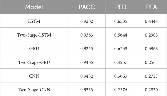
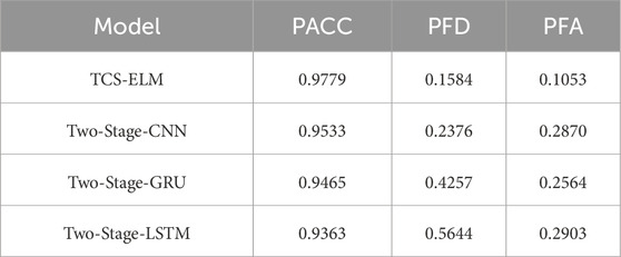
After the training, the model is tested from the test set, and the performance test results of the model are obtained. At the same time, existing Two-Stage models (such as two-stage-LSTM, two-stage-GRU) are tested, which all use the same neural network (such as LSTM or GRU) for positive and negative sample classification and fair classification tasks. The weight coefficient matrix used for model parameter correction is shown in Table 4. Firstly, transient stability evaluation experiments were conducted on the single-stage model and the two-stage model, and the results were recorded and summarized as shown in Table 5.Vertical comparison shows that the two-stage method proposed in this paper outperforms the single-stage method in all indicators, with a significant reduction in misclassification rates and a marked improvement in classification accuracy. This validates the effectiveness of the two-stage model in complex tasks compared to a single model. Figure 5 shows the bar chart comparison of the performance between single-stage and two-stage models.Based on these findings, we further explored the effects of different neural network combinations within the two-stage framework. As such, this paper proposes the TCS-ELM model (Two-Stage Cost-Sensitive Ensemble Learning Model), using CNN for positive and negative sample classification in the first stage and ELM for fair classification in the second stage, fully leveraging CNN’s feature extraction strengths and ELM’s efficient classification capabilities. Table 6 shows the performance testing results of various two-stage models and the proposed TCS-ELM model.Results indicate that the proposed TCS-ELM model, by using CNN in the first stage for stronger feature extraction capabilities and ELM in the second stage for improved classification accuracy, outperforms other two-stage models (such as Two-Stage-LSTM and Two-Stage-GRU) in all indicators, particularly exhibiting higher accuracy and robustness when handling critical samples. This demonstrates that the TCS-ELM model combines the advantages of CNN and ELM in their respective stages, significantly enhancing overall performance. Figure 6 presents the bar chart comparison of the performance between TCS-ELM and other two-stage models.

Table 4

Table 4. Weight coefficient matrix for model parameter modification.

Table 5

Table 5. Comparison of single-stage and two-stage models.

Figure 5

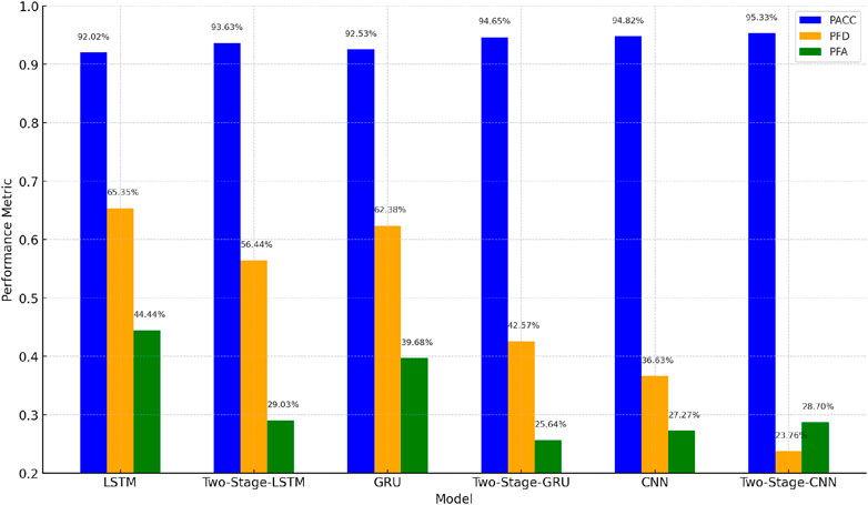
Figure 5. Comparison of performance between single-stage and two-stage models. Model performance improvement: two-stage vs. baseline (LSTM, GRU, CNN).

Table 6

Table 6. Comparison of TCS-ELM with other two-stage models.

Figure 6

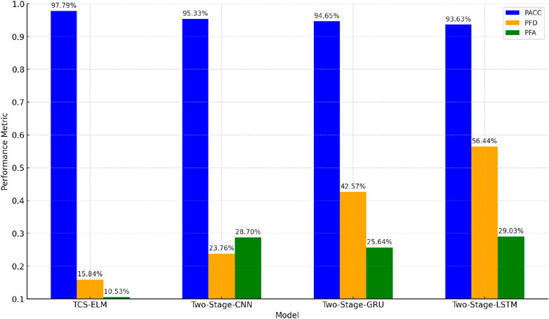
Figure 6. Comparison of performance between single-stage and two-stage models. Performance comparison of 4 deep learning models.

5 Conclusion

In conclusion, the two-stage transient stability assessment model proposed in this paper, which leverages a combination of cost sensitivity and ensemble learning, addresses the key challenge of sample imbalance while exhibiting robust classification capabilities, particularly for hard-to-classify samples. By integrating these advanced techniques, the model demonstrates exceptional performance, achieving high levels of accuracy without compromising the reliability and credibility of the evaluation results.

In contrast to widely used transient stability assessment methods, this model successfully overcomes several of their inherent limitations. Traditional models often struggle to balance speed, accuracy, and reliability, particularly in cases where the data distribution is uneven or where outliers skew the results. The proposed model not only mitigates these issues but also delivers rapid assessments, making it highly efficient for real-time or near-real-time applications. Its ability to provide convincing and trustworthy evaluations further strengthens its utility in practical scenarios where precise and timely decision-making is crucial, such as in power grid operations and other dynamic systems.

By offering a superior balance of speed, accuracy, and evaluation credibility, this model stands out as a significant advancement in the field of transient stability assessment, offering a practical solution that is both scalable and adaptable to diverse operating conditions.

Data availability statement

The raw data supporting the conclusions of this article will be made available by the authors, without undue reservation.

Author contributions

AL: Writing–original draft. YM: Writing–review and editing. DM: Writing–review and editing. ZL: Writing–review and editing. WT: Writing–review and editing. FH: Writing–original draft.

Funding

The author(s) declare that financial support was received for the research, authorship, and/or publication of this article. This study received funding from the Science and Technology Project of China Southern Power Grid Co. Ltd. (ZDKJXM20210063).

Conflict of interest

The authors declare that the research was conducted in the absence of any commercial or financial relationships that could be construed as a potential conflict of interest.

The authors declare that this study received funding from the Science and Technology Project of China Southern Power Grid Co. Ltd. (ZDKJXM20210063). The funder had the following involvement with the study: the study design, the writing of this article.

Publisher’s note

All claims expressed in this article are solely those of the authors and do not necessarily represent those of their affiliated organizations, or those of the publisher, the editors and the reviewers. Any product that may be evaluated in this article, or claim that may be made by its manufacturer, is not guaranteed or endorsed by the publisher.

References

Chen, Q., Lin, N., and Wang, H. (2021). Transient stability assessment model with parallel structure and data augmentation. Int. Trans. Electr. Energy Syst. 31, 12872. doi:10.1002/2050-7038.12872

CrossRef Full Text | Google Scholar

Chen, Q., and Wang, H. (2021). Time-adaptive transient stability assessment based on gated recurrent unit. Int. J. Electr. Power and Energy Syst. 133, 107156. doi:10.1016/j.ijepes.2021.107156

CrossRef Full Text | Google Scholar

Chen, Q., Wang, H., and Lin, N. (2022). Imbalance correction method based on ratio of loss function values for transient stability assessment. CSEE J. Power Energy Syst.

Google Scholar

Du, Y., Hu, Z., and Wang, F. (2021). A hierarchical power system transient stability assessment method considering sample imbalance. Energy Rep. 7, 224–232. doi:10.1016/j.egyr.2021.08.052

CrossRef Full Text | Google Scholar

Fuqiang, L., Shihua, T., Yan, Z., Xiaohui, S., Pengcheng, H., and Zhu, L. (2023). Application of ssa-bp neural network in uav point cloud hole repair. Bull. Surv. Mapp., 130.

Google Scholar

Gu, T., Li, B., Xiao, L., Xu, Y., Mao, J., Yuan, M., et al. (2024). “Power system transient stability assessment based on svm-smote and one-dimensional convolutional neural network,” in 2024 IEEE 2nd international conference on power science and Technology (ICPST) (IEEE), 562–568.

CrossRef Full Text | Google Scholar

Guo, W., Qureshi, N. M. F., Jarwar, M. A., Kim, J., and Shin, D. R. (2023). Ai-oriented smart power system transient stability: the rationality, applications, challenges and future opportunities. Sustain. Energy Technol. Assessments 56, 102990. doi:10.1016/j.seta.2022.102990

CrossRef Full Text | Google Scholar

Ji, J., Wu, J., Wang, Y., Shi, F., and Li, B. (2022). Power system transient voltage stability assessment based on deep residual network. Power Syst. Technol. 46, 2500–2511.

Google Scholar

Jin, W., Zhou, B., Althubiti, S. A., Alsenani, T. R., and Ghoneim, M. E. (2023). Transient stability assessment of power systems using support vector regressor and convolution neural network. Sustain. Comput. Inf. Syst. 37, 100826. doi:10.1016/j.suscom.2022.100826

CrossRef Full Text | Google Scholar

Kesici, M., Mahdi, M., Yaslan, Y., Seker, S., and Genc, I. (2023). A novel integrated framework for real-time prediction of transient instabilities in power systems with their severity levels using deep learning. Sustain. Energy, Grids Netw. 36, 101221. doi:10.1016/j.segan.2023.101221

CrossRef Full Text | Google Scholar

Lee, H., Kim, J., Park, J. H., and Chung, S.-H. (2023). Power system transient stability assessment using convolutional neural network and saliency map. Energies 16, 7743. doi:10.3390/en16237743

CrossRef Full Text | Google Scholar

Li, J., Yang, H., Yan, L., Liu, D., Li, Z., and Xia, Y. (2021). Integrated assessment method for transient stability of power system under sample imbalance. Automation Electr. Power Syst. 45, 34–41.

Google Scholar

Li, Y., Cao, J., Xu, Y., Zhu, L., and Dong, Z. Y. (2024). Deep learning based on transformer architecture for power system short-term voltage stability assessment with class imbalance. Renew. Sustain. Energy Rev. 189, 113913. doi:10.1016/j.rser.2023.113913

CrossRef Full Text | Google Scholar

Lin, J., Cai, R., and Zheng, Z. (2022). A transient stability assessment model based on fault severity assignment. Front. Energy Res. 10, 822729. doi:10.3389/fenrg.2022.822729

CrossRef Full Text | Google Scholar

Liu, F., Wang, X., Li, T., Huang, M., Hu, T., Wen, Y., et al. (2023). An automated and interpretable machine learning scheme for power system transient stability assessment. Energies 16, 1956. doi:10.3390/en16041956

CrossRef Full Text | Google Scholar

Meridji, T., Joós, G., and Restrepo, J. (2023). A power system stability assessment framework using machine-learning. Electr. Power Syst. Res. 216, 108981. doi:10.1016/j.epsr.2022.108981

CrossRef Full Text | Google Scholar

Shao, Z., Wang, Q., Cao, Y., Cai, D., You, Y., and Lu, R. (2024). A novel data-driven lstm-saf model for power systems transient stability assessment. IEEE Trans. Industrial Inf. 20, 9083–9097. doi:10.1109/tii.2024.3379629

CrossRef Full Text | Google Scholar

Shen, J. (2023). Em-tsa: an ensemble machine learning-based transient stability assessment approach for operation of power systems. Math. Biosci. Eng. 20, 8226–8240. doi:10.3934/mbe.2023358

PubMed Abstract | CrossRef Full Text | Google Scholar

Singh, M., and Chauhan, S. (2023). A hybrid-extreme learning machine based ensemble method for online dynamic security assessment of power systems. Electr. Power Syst. Res. 214, 108923. doi:10.1016/j.epsr.2022.108923

CrossRef Full Text | Google Scholar

Wang, H., Hu, L., and Zhang, Y. (2023a). Svm based imbalanced correction method for power systems transient stability evaluation. ISA Trans. 136, 245–253. doi:10.1016/j.isatra.2022.10.039

PubMed Abstract | CrossRef Full Text | Google Scholar

Wang, H., Wang, Q., and Chen, Q. (2020). Transient stability assessment model with improved cost-sensitive method based on the fault severity. IET Generation, Transm. and Distribution 14, 4605–4611. doi:10.1049/iet-gtd.2020.0967

CrossRef Full Text | Google Scholar

Wang, Y., Sun, Y., Li, Y., Feng, C., and Chen, P. (2023b). Risk assessment of power imbalance for power systems with wind power integration considering governor ramp rate of conventional units. Electr. Power Syst. Res. 217, 109111. doi:10.1016/j.epsr.2022.109111

CrossRef Full Text | Google Scholar

Wei Zhang, Q. Z., and Zhang, C. (2024). Spatial-temporal resilience assessment of distribution systems under typhoon coupled with rainstorm events. IEEE Trans. Industrial Inf. doi:10.1109/TII.2024.3450079

CrossRef Full Text | Google Scholar

Wu, J., Zhang, R., Ji, J., and Li, B. (2020). Two-stage transient stability prediction method of power system considering cost of misdetection and false alarm. Automation Electr. Power Syst. 44, 44–56.

Google Scholar

Zhang, L., Hu, X., Li, P., Shi, F., and Yu, Z. (2017). “Elm model for power system transient stability assessment,” in 2017 Chinese automation congress (CAC) (IEEE), 5740–5744.

CrossRef Full Text | Google Scholar

Zhao, D., Xie, J., Wang, C., Wang, H., Jiang, W., and Wang, Y. (2022). On-line transient stability assessment of a power system based on bagging ensemble learning. Power Syst. Prot. control 50, 1–10.

Google Scholar

Zhu, L., Wen, W., Li, J., and Hu, Y. (2023). Integrated data-driven power system transient stability monitoring and enhancement. IEEE Trans. Power Syst. 39, 1797–1809. doi:10.1109/tpwrs.2023.3266387

CrossRef Full Text | Google Scholar