 Anshuo Yao*
 Jiong Chen
- Department of Electrical Engineering, Shanghai University of Electric Power, Shanghai, China
In this study, we propose a CNN-GAN-based real-time processing technique for filtering images of underwater cables used in power systems. This addresses the excessive interference impurities that are frequently observed in images captured by remotely operated vehicles (ROVs). The process begins with the input of the original image into the convolutional neural network (CNN). Subsequently, the training outcomes, which serve as input parameters for the generative adversarial network (GAN), facilitate the filtering process. The system also calculates both the structural similarity index measure (SSIM) and peak signal-to-noise ratio (PSNR), performing model updates via backward propagation. This technique utilizes deep learning technologies to achieve rapid, real-time filtering of underwater cable images. The experimental results reveal that the loss function of the CNN reaches 0.16 with an accuracy of 97.5%, while the loss function of the adversarial GAN network approaches 0.05. Compared with traditional methods such as DDN, JORDOR, RESCAN, and PRENet, the proposed CNN-GAN algorithm exhibits superior performance, as evidenced by the higher PSNR and SSIM values. Specifically, for clear water images, the PSNR reaches 29.86 dB and the SSIM is 0.9045. For severely polluted images, the PSNR is 28.67 dB and the SSIM is 0.8965, while for unevenly illuminated images, the PSNR and SSIM values are 24.37 dB and 0.88, respectively. These enhancements significantly benefit the monitoring and maintenance of power systems.
1 Introduction
Electrical cables are critical power system components that ensure safe and stable operation. The laying of underwater cables serves as a primary channel within the power system infrastructure. During urban cable routing design and construction, it is customary to integrate the developmental needs of the power grid by installing multiple pipelines in a single construction phase. This strategy reserves channels for future expansion of the urban power grid. Over time, the loss of some data due to incomplete cable well information necessitates preliminary exploration and verification when designing new cable routes. This paper considers the deployment of unmanned remotely operated vehicles (ROVs) equipped with cameras, which perform underwater inspections. These inspections are crucial for identifying uncharted cable duct openings and also for detecting malfunctioning cables that may compromise power system stability. Additionally, these surveys aim to preemptively identify potential threats before system malfunctions occur. However, images captured by ROVs often contain significant interference from impurities, which can impede subsequent processes such as edge detection. Therefore, filtering these images is an essential first step for enhancing the accuracy of subsequent analyses.
Traditional filtering techniques such as Wiener filtering (Xiaobin and Li, 2013), median filtering (Bo et al., 2024), and semi−mean filtering (Hanwen et al., 2023) often struggle to address challenges associated with data dimensionality, quality, and complexity. Furthermore, achieving a balance between real-time processing, spatial complexity, and denoising capability remains a significant hurdle. Conventional methods typically require manual tuning of algorithm parameters. This can be time-consuming as adjustments must be made for each image to optimize results. Among these, Buades et al. (2008) developed a non-local mean (NLM) filtering denoising algorithm by enhancing the mean filtering approach. This method leverages the structural similarities across domain graphs, thereby preserving the structural integrity of the original image and enhancing the denoising process.
Machine learning methodologies are broadly categorized into three types: supervised learning, semi-supervised learning, and unsupervised learning. Supervised learning, as described by Xiao et al. (2019), utilizes predefined labels to guide the network in learning features that closely align with the target, facilitating the training of denoising models. The semi-supervised learning approach, highlighted by Mingqiang et al. (2020), exploits learning from paired sinusoidal graphs to supervise the network in understanding feature distributions. In contrast, unsupervised learning methods, outlined by Donghoon et al. (2018), focus on learning data features directly from training samples without relying on matched labels. An example of this is the cyclic generative adversarial network (CinCGAN) proposed by Yuan et al. (2018), which estimates high-resolution images to serve as labels. These labels, alongside specific loss functions, are then utilized to train the model.
With advancements in deep learning technology, numerous generative models such as deep belief networks and variational autoencoders have been studied extensively. Particularly notable are generative adversarial networks (GANs), which have demonstrated excellent capabilities in image restoration by recovering images that have been damaged for various reasons. An early example of influential unsupervised deep neural networks is the stacked self-encoder (SAR) proposed by Hinton and Salakhutdinov (2006), which uses a series of stacked encoders to effectively train models. However, these networks often require repetitive manual tuning of the parameters, prompting a shift towards end-to-end networks such as convolutional neural networks (CNNs), as proposed by Yingjie et al. (2018). Innovative applications of GANs include Divakar and Venkatesh (2017) approach to image denoising, and Wolterink et al. (2017) method for reducing noise in low-dose CT scans by training generators to produce outputs that mimic regular-dose CT images. Yang et al. (2018) enhanced denoising performance by utilizing joint perceptual and adversarial loss, focusing on feature distinctions of pre-trained geometric groups and improving the retention of subjective information. Zhong et al. (2020) integrated a residual structure into their GANs, controlling training by minimizing perceptual loss. Chuan et al. (2018) designed GANs that were fully convolutional networks, employing local features and gradient similarity bias for training control. Addressing the challenge of acquiring paired samples, Jingwen et al. (2018) utilized GANs to generate noisy samples, which were then denoised using CNNs.
Tao et al. (2022) proposed a low-quality image enhancement algorithm based on DDR-GAN, which compared the ESR-GAN and DeBlur GAN-V2 algorithms. This algorithm has higher clarity and richer image details, which is reflected in its improved SSIM and PSNR values. Quanbo et al. (2023) used GAN to improve the resolution of cone-beam computed tomography (CBCT) dental images. The super-resolution network was trained with weak supervision using microtomography images as a reference (Ziyuan, 2020). Conducted research on image denoising and image super-resolution methods based on the GAN network. Eight residual layers were added to the ordinary convolutional network structure so that the main features of the image were not lost during the convolution process. This helped to retain the detail features more effectively during the image super-resolution application. Yuanming et al. (2023) used GAN to enhance underwater images, de-partitioned the original images using an improved white balance algorithm, and completed image feature fusion using a convolutional neural network. Tao et al. (2022) designed a Re-GAN model for the image contamination problem using SAR. They added residual blocks to enhance the ability of noise reduction on the SAR images. Subsequently, the combined loss function in the model preserved the image details more effectively during noise reduction.
While the denoising methods discussed above possess distinct advantages, they also present inherent limitations:
(1) Traditional filtering methods effectively reduce noise, but they process each pixel individually with a filter, which compromises real-time applications. Moreover, these methods primarily focus on pixels within the scope of the filter and often neglect the overall structure of the image. Variations in filter window size may also result in the loss of useful information during the convolution process.
(2) Machine learning-based denoising methods typically require manual tuning of hyperparameters, which introduces uncertainty into the denoising process. Additionally, the reliance on sparse priors and non-local self-similarity priors for natural images may not adequately capture the texture and structure of more complex graphics.
In this paper, we introduce a deep learning-based adaptive system that automates the filtering of underwater cable images. It uses a two-layer nested neural network that combines CNN and GAN, termed CNN-GAN. This system eliminates the need for manual parameter setting, enabling fully automatic optimization of the filtering process. The outer neural network is an unbiased CNN that first receives the original image and passes the derived parameters to the inner GAN network, which then performs the filtering. The filtered image output is evaluated using SSIM and PSNR metrics to facilitate inverse model updating. In practical applications, the system requires only the input of newly captured images to generate optimally filtered results.
2 Convolutional neural network
2.1 Fundamentals of unbiased CNN convolution
The convolutional neural network, as described by Krizhevsky et al. (2014), integrates convolutional computation with a deep structure. A typical CNN comprises three main components: an input layer, a feature learning and representation layer, and a classifier. In this context, the input layer preprocesses multidimensional data, such as the two-dimensional data discussed in this paper. The feature learning and representation layer generally consists of multiple convolutional, activation, and pooling sub-layers. This layer maps input signals to the hidden layer feature space of the CNN, extracting features from the input data. The classifier is often formed by one or more fully connected layers or multilayer perceptron classifiers and is responsible for feature fusion and classification. The convolutional layer includes several sub-layers and forms the core of the CNN. Each convolutional kernel is equivalent to a neuron in a feed-forward neural network and has an associated weight matrix and bias vector. This kernel sweeps through the input features at a set step size, capturing a map of the activated features within its receptive field.
2.1.1 Convolutional layer
The formula for the convolutional layer is (Equation 1):
In this equation, “i” represents the i-th layer of the convolutional network, “k” denotes the index of the feature map in the i-th layer, and “c” signifies the number of convolution kernels in layer i. The symbol “*” represents the convolution operation, “Xi-1(c)” refers to the input feature map of layer i, and “Xi(k)” is the output feature map. The terms “Wi(c,k)” and “Bi(k)” denote the weights and biases of the convolution kernels, respectively.
The inclusion of nonlinear activation functions significantly enhances the feature characterization capability of the CNN model. Notably, the rectified linear unit (ReLU) function exhibits substantial gradient descent capability, effectively solving issues such as gradient explosion and vanishing during the training process. Therefore, the ReLU function is selected as the activation function for the model in this study (Equations 2–4).
2.1.2 Pooling layer
After the convolution operation, the resultant feature map is down-sampled in the pooling layer. The maximum pooling layer segments the feature map into a series of non-overlapping blocks. It selects the maximum value from each block to represent the feature value of that segment, while discarding the other values within the block. Popular pooling methods are depicted in Figure 1.

Figure 1. Schematic diagram of the pooling operation.
The maximum pooling process is (Equation 5):
Here, “Xi(k) (t)” represents the feature map resulting from the convolution operation on the k-th neuron at the i-th layer. The variable “l” denotes the width of the maximum pooled local area, while “Xi+1(k) (i)” is the output feature map following the maximum pooling operation.
2.1.3 Fully connected layer
The fully connected layer constitutes the core component of traditional neural network architectures. In these networks, the fully connected layer maps the input data directly to the output data. However, in convolutional neural networks, the fully connected layer typically follows the convolutional and pooling layers, serving a critical role in classifying the processed features.
The Softmax function is employed in the output layer and is described by the following mathematical expression (Equation 6):
2.1.4 Feature extraction model
The feature extraction model is based on the basic model of ResNet-34, with the addition of the CBAM attention module in front of the average pooling layer, which can weight the features of the convolutional layer and help to retain more information in order to enhance the perception of important information. The added CBAM attention module also optimises the spatial feature learning capability of the ResNet34 model, which in turn improves the accuracy of image classification. The model structure is shown in Figure 2 below.
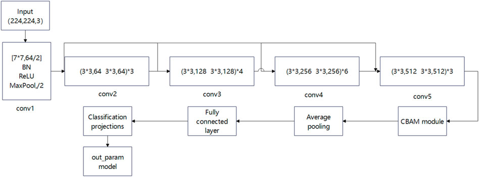
Figure 2. Feature extraction model.
2.2 Parameter selection and principles behind CNN
The learning rate in deep learning is a crucial hyperparameter that determines how fast and in which direction the model updates the weight parameters during training. During each iteration, the model computes the gradient of the loss function with respect to each parameter. The gradient indicates the direction in which the parameters should be adjusted to minimize the loss. The numerical expression is usually (Equation 7):
If the learning rate is set too high, the model parameters may cross the optimal solution in each iteration step, leading to oscillations or divergence. Conversely, if the learning rate is too small, the model will converge to the optimal solution very slowly and may fall into the local minima instead of the global optimal solution. Therefore, in this paper, the Adaptive Moment Estimation (ADAM) optimizer is used to adaptively select the learning rate, thereby accelerating convergence and improving the capability to find the global optimal solution.
The number of iterations per epoch determines the number of times the model needs to be trained. Too many iterations lead to a long program running time, while a smaller number of iterations stops the program too early, before the loss function converges. In the running process of the algorithm in this paper, from the loss function convergence curve to see when epoch reaches a certain value, the loss function convergence. Therefore, in this paper, the number of iterations in the CNN is set to a number that is slightly larger than this epoch value. This ensures that the loss function converges and prevents the program from running too long.
The principle of learning rate and iteration number mentioned here is also applicable to the generative adversarial network described in Section 3.
2.3 CNN training
The outer CNN network is designed to predict two parameters: the learning rate and the number of iterations. These predictions are then utilized to train the inner GAN network. In this study, we employ ADAM, a stochastic optimization algorithm that enhances traditional approaches by adaptively estimating low-order moments. The ADAM optimizer was originally introduced by Kingma and Ba (2014) and it differs from conventional stochastic gradient descent (SGD) or AdaGrad methods. The SGD algorithm maintains a constant learning rate for updating the weights across all parameters, while the AdaGrad algorithm adjusts the learning rate individually for each parameter, which is particularly effective for dealing with sparse gradients. Conversely, the ADAM algorithm dynamically modifies the learning rate based on both first-order and second-order moment estimations of the gradients. This facilitates optimized network structures, accelerated convergence, and enhanced global optimization capabilities. The parameter updating process using the ADAM optimization algorithm is described below (Equations 8–14).
(1) Set the initialization parameters
(2) Calculate the gradient at iteration step t
(3) Update the first-order moment estimate gradient mt
Update the second-order moments to estimate the gradient vt
(4) Update the gradient of the modified first-order moment estimate
Update the gradient of the modified second-order moment estimate.
(5) Update the parameters:
(6) If t>tmax then return the updated parameters, if otherwise return the first step.
In the above equations, “m” and “v” denote the first and second-order moments of the gradient, respectively, while “α” represents the learning rate. The learning rate determines how quickly the model updates its parameters during training, directly influencing the convergence speed and quality. The learning rate is typically set to 0.0001. The parameters “β₁” and “β₂” are the decay rates for the first and second-order moments, respectively, with default values of 0.9 and 0.999 during model training.
2.4 CNN cross-entropy loss function
In the CNN, the loss function quantifies the deviation of the network output from the labeled result, serving as a crucial component in the backpropagation process for updating gradients. The goal of continuous training and parameterization in the CNN is to minimize the loss function and learn the optimal model. The cross-entropy loss function is commonly employed to minimize the difference between the predicted probability distribution and the true probability distribution, thereby making the predictions as accurate as possible. For image classification tasks, a combination of the Softmax function and cross-entropy is often utilized as the loss function. The Softmax function is particularly effective in multi-category classification tasks, as it maps the output of multiple neurons, y = f(x), to the interval [0, 1], resulting in a predicted probability distribution. This distribution indicates the likelihood of the input belonging to each category, facilitating multi-class classification.
Given a probability distribution where “i” denotes the i-th element, the Softmax value of the element is calculated as follows (Equation 15):
The cross-entropy loss function, frequently used in classification tasks, is defined by the following formula (Equation 16):
where p(x) denotes the real probability distribution and q(x) represents the predicted probability distribution. For a known outcome, p(x) typically takes the form of a one-hot encoded vector, such as [0,0,0,0,0.1,0,0,0,0], indicating a unique classification. Conversely, q(x) indicates the predicted probability of belonging to each classification category.
3 Generative adversarial networks
Generative adversarial networks are a powerful class of neural networks that are used for unsupervised learning. GANs consist of two competing models: the generator (G) and the discriminator (D). The generator creates fake data samples (e.g., images, audio) and attempts to deceive the discriminator, while the task of the discriminator is to distinguish between real and fake samples. Both the generator and discriminator compete against each other during the training phase, and this iterative process enables both models to improve their performance over time. The structure of the GAN network is depicted in Figure 3.
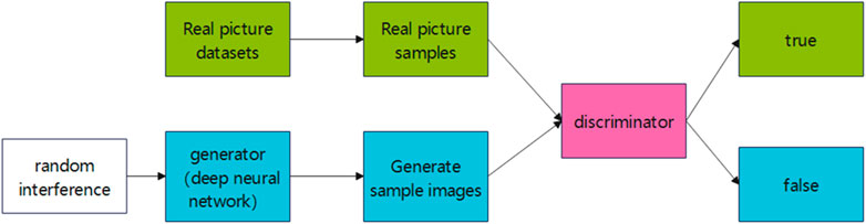
Figure 3. GAN schematic diagram.
3.1 GAN training process
The GAN training process involves the following steps:
1. Randomly generate a set of latent vectors z and use the generator to produce a set of fake data.
2. Train the discriminator using a set of real data and the generated fake data as inputs.
3. Generate a new set of fake data using the generator and continue training the discriminator.
4. Repeat Steps 2 and 3 until the generator produces fake data that has a similar distribution to the real data.
The images produced by the generator in the previous round are combined with the real images to form a dataset x. Labels are assigned such that fake images correspond to 0 and real images to 1. The discriminator then processes the dataset x to produce a score between 0 and 1, representing the probability that an image is real. The loss function, based on the score and the true label y, is used for gradient backpropagation to update the network parameters. The GAN training process is shown in Figure 4.
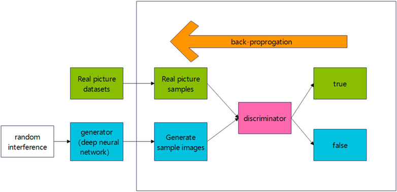
Figure 4. GAN training process.
At this stage, the generator G and the discriminator D are considered a unified system. In this paper, it is referred to as the DG system, and the output of this system is still the score. By inputting a set of random vectors, G generates an image, which D then evaluates. This constitutes the forward process of the DG system. The ultimate optimization goal of the DG system is to maximize the score, ideally reaching a value of 1, which indicates that the generated image is indistinguishable from a real image. The Retraining generator is shown in Figure 5.
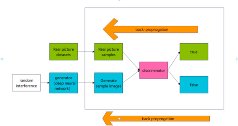
Figure 5. Retraining generator.
3.2 Parameter selection and principles behind GAN
In addition to the learning rate and the number of iterations, there are several other parameters in the GAN, including batch size (batch_size), number of CPUs used for data loading (n_cpu), dimensionality of the random vectors (latent_dim), and so on. However, the main parameters that have a decisive impact on the training results of the GAN remain the learning rate and the number of iterations. Therefore, in the algorithm design process of this paper, only two CNN output parameters are used to maximize the efficiency of the procedure.
3.3 Objective function
In discriminative networks, there are two types of input data: one from real samples and one from generative networks. Their binary cross-entropy loss is (Equation 17):
In the above equation, x is drawn from the true distribution Pdata, while D(x) reflects the possibility that the discriminative network assigns x to Pdata. The variable z denotes the input random data for the generator network and PZ represents the probability distribution of the random data. The term G(z) refers to the generated data, and D (G(z)) is the probability that the discriminative network assigns the generated sample to Pdata. Based on the aggregate of the cross-entropy losses for real and generated data, the optimization objective function can be expressed as (Equation 18):
In the training optimization phase of the GAN, the discriminative network aims to maximize the objective function. This ensures that the prediction probability D(x) for the real sample x converges to the true value, while the prediction probability D (G(z)) for the generated sample G(z) converges to the false value. Simultaneously, the purpose of the generative network is to minimize the objective function. Since log D(x) is independent of the generative network, the primary goal is to minimize log(1−D (G(z))). This adjustment promotes the convergence of D (G(z)) to the true value.
3.4 Overall program framework
The overall framework of the system in this study integrates two algorithms as the outer and inner frameworks. The outer layer utilizes a CNN algorithm that determines the optimal parameters of the GAN, while the inner layer employs the GAN to generate the final filtered image. The outer layer CNN uses 5,000 submerged images of cable wells captured by ROVs as the training dataset. The outputs of this CNN are the learning rate and the number of iterations required for the two GAN networks. The training procedure is implemented using Python, where the dataset is randomly split into training and test sets using the random_split method, allocating 80% for training and 20% for testing. The 5,000 images that serve as the training set are used to ascertain the parameters applied to the GAN. These images are entered into the CNN, which subsequently determines the input parameters for the GAN during subsequent training. Without the nesting of the outer CNN, the training GAN model requires manually specified parameters. This paper focuses on two fundamental parameters: the number of iterations and the learning rate. The GAN incorporates a model that automates the filtering of the input images based on these parameters. To evaluate the filtering effect of the final image, we employ frame-by-frame screenshots of videos to conduct both subjective and objective assessments of underwater images under various lighting conditions, scenes, and color shades. Figure 6 illustrates the overall program framework.
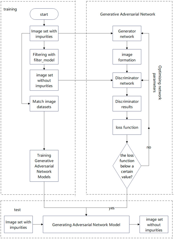
Figure 6. Overall program framework.
3.5 Image evaluation indicators
Subjective evaluation of image denoising performance can be quantitatively determined using the peak signal-to-noise ratio (PSNR) and structural similarity (SSIM) metrics (Liu, 2023; Siyu, 2023; Lihua, 2023).
(1) PSNR is one of the most widely used evaluation metrics. A higher PSNR value indicates superior processed image quality. The formula for PSNR is (Equation 19):
where max2 is the maximum possible pixel value of the original image I, usually 255. MSE denotes the mean square error between the original image I of size M*N and the processed image K, calculated as (Equation 20):
(2) SSIM is a metric that measures the structural similarities between two images, modeling image distortion as a combination of three factors: correlation loss, luminance distortion, and contrast distortion. SSIM is calculated as follows (Equation 21):
SSIM values lie between 0 and 1, with higher values indicating greater similarity and better correlation between the denoised image and the reference image.
4 Experiments
4.1 Outer CNN training results
The experimental study in this paper uses images of real cable duct openings captured in situ using an unmanned ROV. The samples include frames from multiple video recordings in clear water, heavily polluted water, and uneven lighting conditions. Python is used as the programming platform, with an NVIDIA GeForce RTX4090 and an Intel(R) Core i7-13700 KF CPU. For the Conv2d 2D convolutional layer, “batch_size” is set to 3, the convolutional kernel size is 7*7, the step size is 2, and the padding is set to 3. The proposed convolutional residual neural network (CNN) model has five layers in total, and the number of neurons in the residual module of Layer1, Layer2, Layer3, Layer4, and the output layer is 64, 128, 256, and 512. A total of 1,000 epochs of training are performed to obtain the loss function image. The step sizes of Layer2, Layer3, and Layer4 are all set to 2. The size of the sampling window under the maximum pooling layer is set to 3*3, and the modified current unit ReLU is selected as the activation function.
The sizes of the images used in this paper are 1920*1,080, which are cropped to 180*180*64 size and input to the CNN for convolution pooling work. After the first convolution, the output channel changes from 64 to 128, and the image size becomes 180*180*128. Next, following the first pooling, the pooling step is set to 2 and the image size becomes 90*90*128. In the second convolution, the output channel changes from 128 to 256, and the image size becomes 90*90*256. In the second pooling, with a step size of 2, the image size becomes 45*45*256. On entering the third convolution, the output channel changes from 256 to 512, and the image size becomes 45*45*512. The step size of the third pooling is 2, so the image size becomes 22*22*512. This output from the final pooling becomes the input to the fully-connected layer. After the fully-connected layer, the first layer contains 1,024 neurons, while the second layer has 10 neurons. The neuron nodes pass through the Softmax layer to generate the probability of each category corresponding to its respective goal. Finally, the outparam model is added at the end of the CNN procedure. Its function is to calculate the probability by detecting the similarity between the feature image of the test set and the feature image of the training set by CNN. Ultimately, it generates the parameters of the GAN corresponding to the feature image of the test set.
The dataset is divided in an 80:20 ratio into training and testing sets. The CNN loss function optimized using the ADAM optimizer appears in Figure 7, and its accuracy on the corresponding test set is presented in Figure 8.
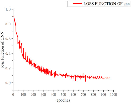
Figure 7. CNN loss function after ADAM optimization.

Figure 8. Accuracy of the corresponding test set after ADAM optimization.
As Figures 7, 8 indicate, after applying the ADAM optimizer, the loss function of the CNN converges to 0.16, while the corresponding accuracy ultimately reaches 97.5%.
4.2 GAN parameters
The analyses in Section 4.1 confirm that the CNN training achieves excellent results. Therefore, the input parameters derived from the CNN for the GAN are considered optimal. This paper focuses on two GAN parameters: the learning rate and the number of epochs. The final results indicate that the optimal learning rate is 0.0001 and the number of iterations (epochs) is 102. The fitted curves for these parameters are shown in Figures 9, 10, respectively.
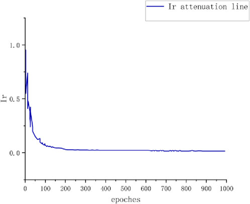
Figure 9. Learning rate decay fitting curve.
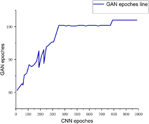
Figure 10. GAN iteration count epoch curve.
The above graphs show that after training the CNN neural network, the output values for the learning rate and the number of iterations converge at 0.0001 and 102, respectively. These two values are used as the input parameters for the inner GAN neural network.
4.3 GAN training
The input parameters for the GAN are derived from the CNN in the previous section and are used by the inner GAN for filtering. The GAN outputs two metrics for image quality assessment: SSIM and PSNR. In this paper, we compare the proposed model with other conventional methods: DNN (Lihua, 2023), JORDER (Yang et al., 2017), RESCAN (Li et al., 2018), and PRENet (Dongwei et al., 2019). The comparison is conducted under three different scenarios: clear water, heavily polluted water, and uneven illumination.
The loss function convergence curve of the GAN during the training process is shown in Figure 11. It reveals that the loss function of the GAN ultimately converges to 0.05, indicating a clear convergence trend.
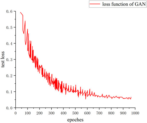
Figure 11. GAN loss function.
The underwater images in good water quality conditions are designated as Test1. Figures 12A–F presents the subjective filtering effects of the Test1 dataset. The figure shows that the DDN algorithm does not effectively remove impurities, resulting in unclear images. The JORDER algorithm shows relatively good impurity removal but still leaves some residual impurities. Although the RESCAN algorithm successfully removes impurities, it causes image smoothing and blurring in detail processing. Besides, the PERNet algorithm exhibits slight deficiencies in background color processing. In contrast, our proposed method effectively removes sparse impurities while preserving the background information.
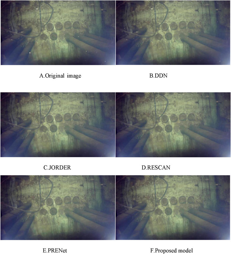
Figure 12. Good water quality.
For the Test1 dataset, we also employ the SSIM and PSNR objective metrics to assess the filtering effects. The results are presented in Table 1.
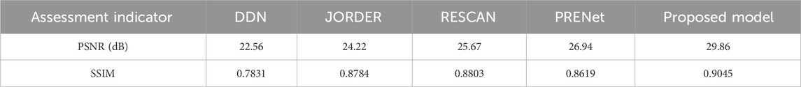
Table 1. Good water quality.
Figures 13A–F shows the subjective filtering effect of the Test2 dataset, which comprises images in heavily polluted water. According to the figure, the DNN presents more visible impurities, while JORDER and PRENet exhibit some residual impurities and somewhat blurred backgrounds. A comparison of the modified images confirms that our proposed method handles images with dense impurities more effectively and also performs better in detailed image processing.
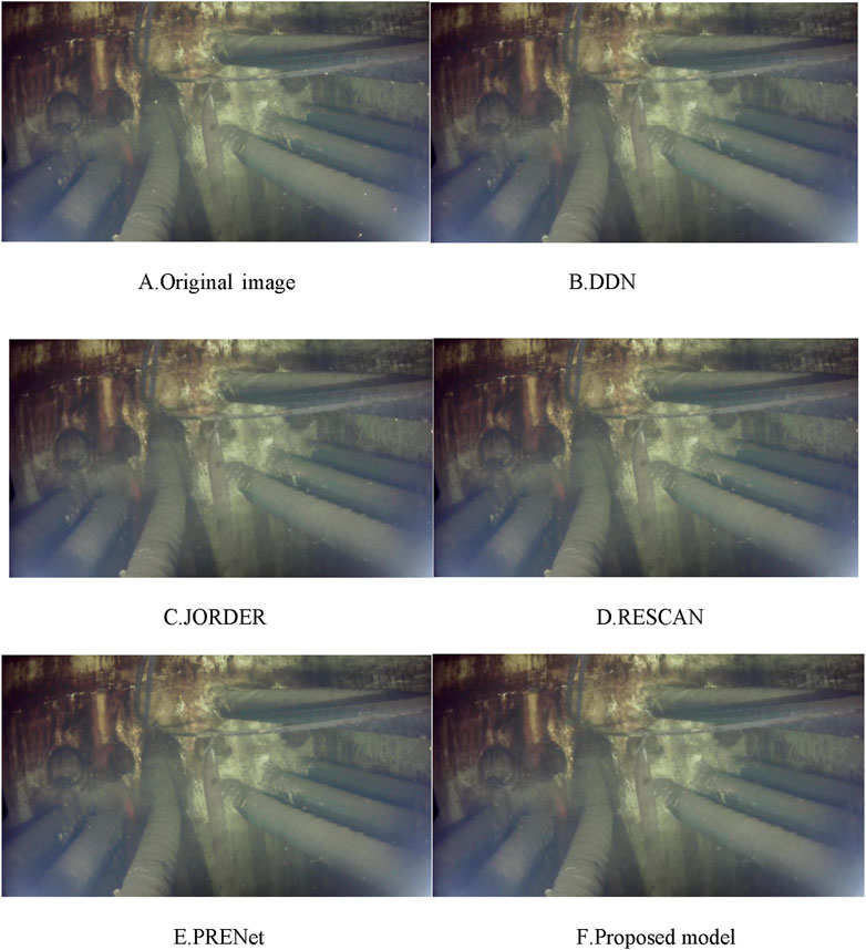
Figure 13. Heavily polluted water.
The results of the SSIM and PSNR objective evaluation metrics for the Test2 dataset are shown in Table 2.
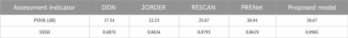
Table 2. Heavily polluted water.
The Test3 dataset represents images with uneven illumination, and Figures 14A–F illustrates the subjective filtering effects for this dataset. The experimental results demonstrate that the proposed algorithm achieves 89% accuracy in the SSIM index, with a PSNR value of 28.67 dB. This confirms that our algorithm effectively removes impurities while preserving image details, enhancing clarity, and maintaining the original colors to some extent.
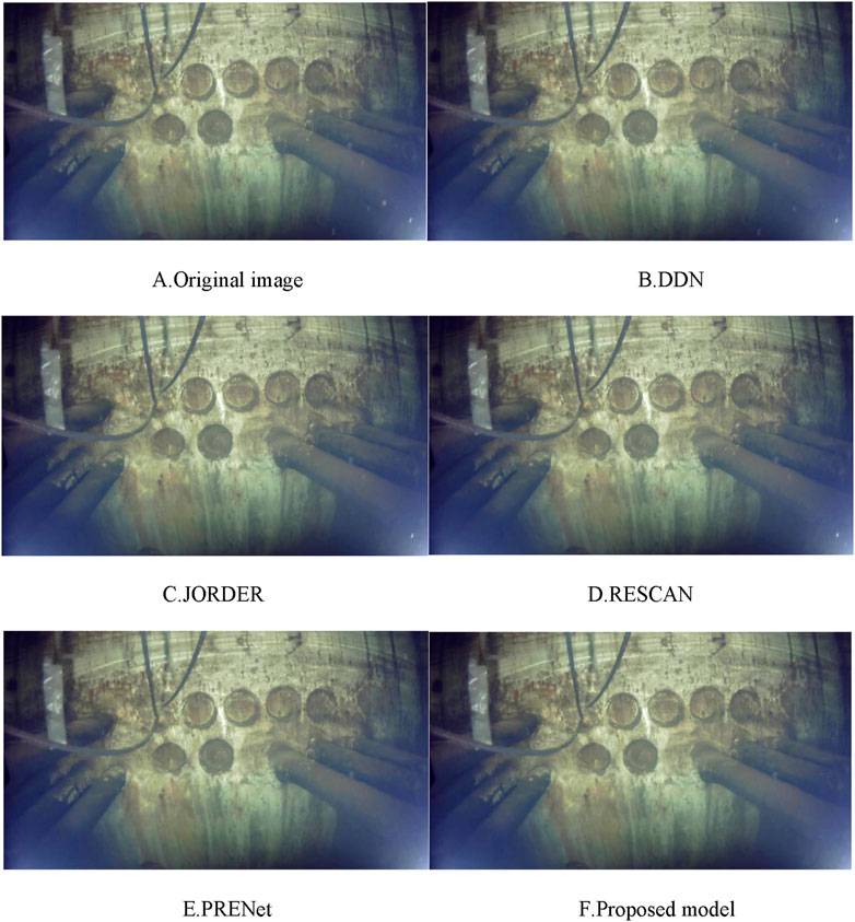
Figure 14. Uneven illumination.
For the Test3 dataset, the results of the objective evaluation metrics SSIM and PSNR are shown in Table 3.
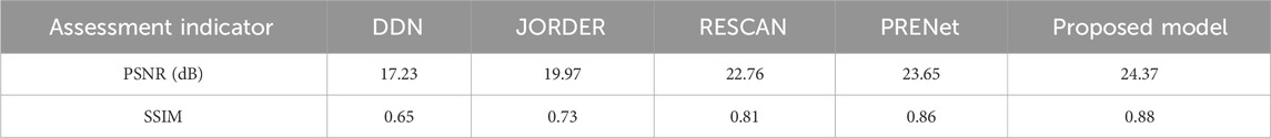
Table 3. Uneven illumination.
5 Conclusion
The underwater image filtering method based on CNN-GAN proposed in this paper avoids traditional manually-tuned filtering parameters in favor of deep learning adaptive filtering. This approach allows for the automatic filtering of various images without the need to set the parameters, thereby enabling direct input of images into the dataset. This method addresses the issue of unclear and poor-quality images in underwater cable pipeline surveys, facilitating straightforward follow-up inspections and more accurate results. The CNN neural network achieves a loss function value of 0.16 and an accuracy rate of 97.5%, while the loss function of the GAN adversarial network converges to approximately 0.05. Compared to traditional methods such as DDN, JORDER, RESCAN, and PRENet, the proposed CNN-GAN neural network is more suitable for underwater cable pipeline inspections. The CNN-GAN algorithm yields higher evaluation indexes for both PSNR and SSIM. Specifically, for images in clear water, the PSNR value increases to 29.86 dB and the SSIM value is 0.9045. For images in severely polluted water, the PSNR and SSIM values are 28.67 dB and 0.8965, respectively. In uneven lighting, the PSNR value is 24.37 dB, while the SSIM value is 0.88. These improvements result in a better underwater image filtering effect, contributing to the stability of the power system.
In future research, we will consider making improvements to the study in the following three areas:
(1) The computing time of the proposed algorithm is long, with an average training time of 15 min using an RTX4090 graphics card. In future research, we will consider reducing the number of epochs, using GAN architectures with faster convergence speeds, and enhancing the real-time nature of the algorithm.
(2) Currently, in addition to the traditional GAN architecture, there are other types of GAN architectures, such as the deep convolutional generative adversarial network (DCGAN), CycleGAN, FUnIE-GAN, etc. We can further improve the GAN architecture in this paper and compare it with existing GAN architectures to obtain a better filtering effect of underwater images.
(3) The dataset trained in this paper only utilizes images of underwater cable vents captured by ROVs, but the proposed algorithm can be applied to a wider range of subjects in subsequent research. For instance, it can be applied to submarine cable images captured on the seabed, because the seabed contains a lot of debris, algae, and other objects that can interfere with the target. Our image filtering algorithm produces clearer and more complete images, which helps relevant staff to perform regular inspections and repairs of submarine cables and more effectively maintain power system stability. Additionally, the application range of this image-filtering technique is very broad, so it can be applied in non-electrical areas, such as submarine geological exploration and other work. Most marine mineral resources are located in the seabed, including oil, natural gas, and metals, so the exploration and development of seabed geology is very significant. Our proposed algorithm can filter seabed images in real time, thereby improving the efficiency of geological exploration.
Data availability statement
The original contributions presented in the study are included in the article/supplementary material, further inquiries can be directed to the corresponding author.
Author contributions
AY: Conceptualization, Data curation, Formal Analysis, Funding acquisition, Investigation, Methodology, Project administration, Resources, Software, Supervision, Validation, Visualization, Writing–original draft, Writing–review and editing. JC: Writing–original draft, Writing–review and editing.
Funding
The author(s) declare that no financial support was received for the research, authorship, and/or publication of this article.
Conflict of interest
The authors declare that the research was conducted in the absence of any commercial or financial relationships that could be construed as a potential conflict of interest.
Publisher’s note
All claims expressed in this article are solely those of the authors and do not necessarily represent those of their affiliated organizations, or those of the publisher, the editors and the reviewers. Any product that may be evaluated in this article, or claim that may be made by its manufacturer, is not guaranteed or endorsed by the publisher.
References
Bo, Z., Jie, Z., Wei, L., and Yi, Z. (2024). Research on fast median filter algorithm based on pointer sorting. Mach. Build. and Automation 53 (02), 175–178+242. doi:10.19344/j.cnki.issn1671-5276.2024.02.037
Buades, A., Coll, B., and Morel, J. M. (2008). Nonlocal image and movie denoising. Int. J. od Comput. Vis. 76 (2), 123–139. doi:10.1007/s11263-007-0052-1
Chuan, X., Yongchao, W., Zhijie, L., Qiulan, Z., Fei, Q., and Lei, Z. (2018). Monte Carlo noise removal algorithm based on adversarial generative. Network 31 (11), 1047–1060. doi:10.16451/j.cnki.issn1003-6059.201811009
Divakar, N., and Venkatesh Babu, R. (2017). “Image denoising via CNNs: an adversarial approach,” in Proceedings of the IEEE Conference on Computer Vision and Pattern Recognition Workshops, 80–87.
Donghoon, L., Sangdoo, Y., Sungjoon, C., Hwiyeon, Y., Ming-Hsuan, Y., and Songhwai, O. (2018). “Unsupervised holistic image generation from key local patches,” in Proceedings of the European conference on computer vision (ECCV), Cham, 19–35.
Dongwei, R., Wangmeng, Z., Qinghua, H., Pengfei, Z., and Deyu, M. (2019). “Progressive image deraining networks: a better and simpler baseline,” in Conference on Computer Vision and Pattern Recognition (CVPR), IEEE.
Hanwen, H., Meng, W., Weiping, C., Zonglin, L., and Miaomiao, C. (2023). An image duet-filtering and feature enhancement algorithm for underwater visual SLAM. SLAM 45, 197–206. doi:10.13973/j.cnki.robot.210406
Hinton, G. E., and Salakhutdinov, R. R. (2006). Reducing the dimensionality of data with neural networks. science 313 (5786), 504–507. doi:10.1126/science.1127647
Jingwen, C., Jiawei, C., Hongyang, C., and Ming, Y. (2018). “Image blind denoising with generative adversarial network based noise modeling,” in Proceedings of the IEEE conference on computer vision and pattern recognition, Salt Lake City, UT, USA, 3155–3164.
Kingma, D., and Ba, J. (2014). Adam: a method for stochastic optimization. Comput. Sci. doi:10.48550/arXiv.1412.6980
Krizhevsky, A., Sutskever, I., and Hinton, G. E. (2014). Imagenet classification with deep convolutional neural networks. Commun. ACM 60, 84–90. doi:10.1145/3065386
Li, X., Wu, J., Lin, Z., Liu, H., and Zha, H. (2018). “Recurrent squeeze-and-excitation context aggregation net for single image deraining,” in Proceedingsof the 2018 European Conference on Computer Vision, Springer, Cham, 262–277. doi:10.1007/978-3-030-01234-2_16
Lihua, S. (2023). Study on reconstruction of speckle pattern for the scalar and vector optical fields passing through a scattering medium based on deep learning. [master’s thesis]. Zhejiang, China: Zhejiang SCI-TECH University. doi:10.27786/d.cnki.gzjlg.2023.000913
Liu, H. (2023). Research and hardware implementation of single blind image motion blur removal algorithm based on deep learning. [master’s thesis]. Xi’An, China: XI’AN University of Technology. doi:10.27398/d.cnki.gxalu.2023.000616
Mingqiang, M., Sui, L., Lisha, Y., Danyang, L., Manman, Z., Qi, G., et al. (2020). “Semi-supervised learned sinogram restoration network for low-dose CT image reconstruction,” in Medical Imaging 2020: Physics of Medical Imaging, SPIE, 67–73.11312.
Quanbo, S., Yangke, L., Yeying, F., Shuyi, L., and Yuanfeng, Z. (2023). CBCT tooth images super-resolution method based on GAN prior. J. Computer-Aided Des. and Comput. Graph. 35 (11), 1751–1759. doi:10.3724/SP.J.1089.2023.19756
Siyu, C. (2023). Research and hardware implementation of single image super-resolution reconstruction algorithm based on deep learning. [master’s thesis]. Xi’An, China: XI’AN University of Technology. doi:10.27398/d.cnki.gxalu.2023.000946
Tao, X., Jiansheng, G., Xiaofeng, Z., Taoyong, G., and Boxin, Z. (2022). SAR image noise reduction model based on GAN. Electron. Opt. Control 29 (09), 48–52. doi:10.3969/j.issn.1671-637X.2022.09.010
Wenhan, Y., Robby, T., Jiashi, F., Jiaying, L., Zongming, G., and Shuicheng, Y. (2017). “Deep joint rain detection and removal from a single image,” in IEEE Conference on Computer Vision and Pattern Recognition (CVPR), IEEE, 1357–1366.
Wolterink, J. M., Leiner, T., Viergever, M. A., and Isgum, I. (2017). Generative adversarial networks for noise reduction in low-dose CT. IEEE Trans. Med. imaging 36 (12), 2536–2545. doi:10.1109/tmi.2017.2708987
Xiao, X., Xiong, N. N., Lai, J., Wang, C. D., Sun, Z., and Yan, J. (2019). A local consensus index scheme for random-valued impulse noise detection systems. IEEE Trans. Syst. Man, Cybern. Syst. 51 (6), 3412–3428. doi:10.1109/tsmc.2019.2925886
Xiaobin, H., and Li, Y. (2013). Application of impproved Wiener Filter in image restoration. J. Suzhou Univ. 28 (10), 44–46. doi:10.3969/j.issn.1673-2003.2013.10.013
Yang, Q., Yan, P., Zhang, Y., Yu, H., Shi, Y., Mou, X., et al. (2018). Low-dose CT image denoising using a generative adversarial network with Wasserstein distance and perceptual loss. IEEE Trans. Med. imaging 37 (6), 1348–1357. doi:10.1109/tmi.2018.2827462
Yingjie, Y., Xiaohe, W., Lei, Z., Shiguang, S., and Wangmeng, Z. (2018). “Joint representation and truncated inference learning for correlation filter based tracking,” in Proceedings of the European conference on computer vision (ECCV), 552–567.
Yuan, Y., Siyuan, L., Jiawei, Z., Yongbing, Z., Chao, D., and Liang, L. (2018). “Unsupervised image super-resolution using cycle-in-cycle generative adversarial networks,” in Proceedings of the IEEE Conference on Computer Vision and Pattern Recognition Workshops, 701–710.
Yuanming, D., Surui, L., and Yang, Y. (2023). Underwater image enhancement based on generative adversarial networks. Ship Science Technology 45 (22), 143–147. doi:10.3404/j.issn.1672-7649.2023.22.027
Zhong, Y., Liu, L., Zhao, D., and Li, H. (2020). A generative adversarial network for image denoising. Multimedia Tools Appl. 79, 16517–16529. doi:10.1007/s11042-019-7556-x
Keywords: power system, underwater cable, CNN-GAN, deep learning, image filtering
Citation: Yao A and Chen J (2024) Research on improved underwater cable image processing technique based on CNN-GAN. Front. Energy Res. 12:1452270. doi: 10.3389/fenrg.2024.1452270
Received: 20 June 2024; Accepted: 05 September 2024;
Published: 19 September 2024.
Edited by:
Feng Liu, Nanjing Tech University, ChinaReviewed by:
Fang-Rong Hsu, Feng Chia University, TaiwanYuanjiang Li, Jiangsu University of Science and Technology, China
Copyright © 2024 Yao and Chen. This is an open-access article distributed under the terms of the Creative Commons Attribution License (CC BY). The use, distribution or reproduction in other forums is permitted, provided the original author(s) and the copyright owner(s) are credited and that the original publication in this journal is cited, in accordance with accepted academic practice. No use, distribution or reproduction is permitted which does not comply with these terms.
*Correspondence: Anshuo Yao, MTgzMjEzMDI0MjdAMTYzLmNvbQ==