A hybrid model based on the photovoltaic conversion model and artificial neural network model for short-term photovoltaic power forecasting

Photovoltaic (PV) power is greatly uncertain due to the random meteorological parameters. Therefore, accurate PV power forecasting results are significant for the dispatching of power and improving of system stability. This paper proposes a hybrid forecasting model for one-day-ahead PV power forecasting under different cloud amount conditions. The proposed model consists of an improved artificial neural network (ANN) algorithm and a PV power conversion model. First, the ANN model is designed to forecast the plane of array (POA) irradiance and ambient temperature. Backpropagation, gradient descent, and L2 regularization methods are applied in the structure of the ANN model to achieve the best weights, improve the prediction accuracy, and alleviate the effect of overfitting. Second, the PV power conversion model employs the forecasted results of POA irradiance and ambient temperature to determine the PV power produced by a PV module. In addition to the basic temperature factor, environmental efficiency and a reflection efficiency are incorporated into the conversion model to account for real PV module losses. The performance of the proposed model is validated with real weather and PV power data from Alice Springs and Climate Data Store. Results indicate that the model improves the forecast accuracy compared to four benchmark models. Specifically, it reduces root mean square error (RMSE) and normalized RMSE (nRMSE) by up to 25% under cloudy conditions and offers a 3% shorter training time compared to extreme gradient boosting.

1 Introduction

Solar energy is the largest renewable energy resource available on our planet. Therefore, power generation using solar energy is one of the priorities of current research on green technology. Accurate forecasts of photovoltaic (PV) power production can not only enhance the PV penetration rate within the electricity grid but also aid in grid dispatch and operation (Visser et al., 2022). However, PV power generation has strong randomness, intermittence, and volatility caused by many uncertain factors such as temperature, cloud, and humidity Therefore, the uncertainty of PV power poses huge challenges to the security and reliability of power system operations (Ma et al., 2021). Consequently, in order to reduce the disturbance caused by the stochasticity of power generation and ensure the stable operation of the grid in large-scale PV penetration, an accurate prediction model should be built (Ge et al., 2020). There are three popular methods in short-term PV power forecasting: physical methods, statistical methods, and hybrid methods. The physical methods describe the conversion relationship between solar radiation and PV power through mathematical models (De la Parra et al., 2017). For physical methods, the weather parameters are obtained from the numerical weather prediction (NWP) or the weather stations surrounding the PV plants. A physical model is established to calculate the maximum power and the annual output produced by four thin-film PV modules based on the datasets of electrical and meteorological parameters in sunny inland climates (Torres-Ramírez et al., 2014). However, in harsh weather conditions, physical models are disturbed by various uncertain factors in the environment, which leads to inaccurate forecasting (Mustafa et al., 2020). The statistical methods are suitable for the short-term forecasting horizon, which build the PV forecasting model based on the relationship between the input and the output layers. Three main models of statistical methods are time-series models, regression models, and neural network models. Time-series methods have been popular for relatively stationary sequence prediction. The most common model is an autoregressive integrated moving average (ARIMA) (Bouzerdoum et al., 2013), which is improved by the autoregressive (AR) model and autoregressive moving average (ARMA) model. In regression models, support vector regression (SVR) stands out as a classic model that utilizes the same input features and datasets, delivering superior performance in forecasting stability. However, it demands a significant amount of data for training (Wolff et al., 2020). Many neural network methods are applied to PV power output prediction with the deep development of artificial intelligence (AI) techniques. The recurrent neural network (RNN) algorithm is a neural network model that can find the connecting link in factors and accommodate dependencies among continuous time steps (Gao et al., 2019). A long short-term memory recurrent neural network (LSTM-RNN) is established to forecast PV power, and the forecasting values are updated based on the time correlation principles (Wang et al., 2019). The artificial neural network (ANN) has been identified as an appealing technique for one-day-ahead forecasting due to its capability to establish relationships between input and output datasets and its ability to integrate solar power data with other meteorological data (Bishop, 1995). The ANN model is a popular nonlinear data-driven model that is based on the pattern model rather than a predefined math model. In addition, compared with other models, it is easier to build models that are more cost effective and consume less time (Barbieri et al., 2017). The ANN is successfully used for 24-hour solar irradiance forecasting with superior performance on sunny and cloudy days (Mellit and Pavan, 2010). ANNs trained with datasets reduce the error of 12–18 h ahead of global horizontal irradiance forecasting by approximately 15% (Martins et al., 2012). Moreover, the ANN model is composed of interconnected ANN layers that are trained via a supervised learning technique and applied for power output or irradiance forecasting (Zhao et al., 2023). ANN models are designed to forecast daily irradiance by using GHI ground data, air temperature, and other meteorological parameters (Diagne et al., 2009). However, for ANN models, as the model structure becomes complex, its fitness will decrease. Additionally, the selection of hyperparameters can also have an impact on the prediction accuracy.

Hybrid methods aim to improve the forecasting performance by combining different approaches or targeting multiple time horizons. In fact, increasing number of research works indicates that hybrid methods often outperform single methods in many aspects. A hybrid model is applied to optimize the prediction value forecasted by an ANN model on 4 sunny days (Diagne et al., 2009). A hybrid model that combines a spatiotemporal forecasting approach with a relatively accurate physical model is employed to achieve impressive prediction values in various positions (Tascikaraoglu Sanandaj et al., 2016). Although the hybrid model can provide a more accurate prediction, distortion can occur in bad weather.

With the further increase in renewable energy grid-connection requirements, accurate forecasting in the event of weather changes has become increasingly important. In this paper, to address the complexity of the forecasting environment, the statistical and physical models in the hybrid approach were enhanced. Since statistical models have a much greater impact on the results than physical models in hybrid models, three different methods have been applied to improve the model fit, forecasting accuracy, and computational speed of the ANN, particularly to compensate for the non-stationary sequences caused by weather changes. Furthermore, environmental factors were incorporated into the physical model to enhance the conversion formula. As a result, a hybrid model combining the refined ANN forecasting model with a well-established PV conversion model is proposed to achieve more precise PV power forecasting. The hybrid method can significantly enhance the overall integrity of both the PV prediction process and the forecasting results compared with direct methods. The main contributions of this paper are as follows:

1) First, this paper proposes a hybrid model consisting of an ANN model and a PV conversion model for PV power forecasting. In the PV conversion model, the temperature derating factor, the environmental coefficient, and the reflection coefficient are taken into consideration.

2) Subsequently, this paper improves the ANN model. L2 regularization is applied to control the model structure complexity and prevent overfitting. The backpropagation algorithm is used to find the best weight. In addition, the random Gaussian distribution is introduced for weighs initialization to reduce the computation and improve the accuracy.

3) Furthermore, this paper adds the cloud amount parameters with three different locations into forecasting for reflecting the importance and impact of the cloud amount on irradiance, especially in variable weather conditions.

4) At last, to further determine the environmental conditions of prediction, this paper not only divides the weather conditions of datasets but also categorizes the weather classification based on the weather variability and cloud cover.

The remainder of this paper is organized as follows. Section 2 describes the PV conversion model. The weather classification is provided in Section 3, and the proposed forecasting method is introduced in Section 4. In Section 5, the proposed method is applied to obtain the forecasting values, and the results are compared with real data and benchmark models. Some concluding remarks and outlines of the possible extensions are included in Section 6.

2 Photovoltaic conversion model

To define the PV conversion model, the factors affecting PV module behavior are considered. Although the conversion model is mainly influenced by operating temperature, environmental and physical factors also affect its results. Therefore, the derating factors for basic temperature, environmental efficiency, and reflection efficiency are incorporated into the conversion formula. The derating factor for operating temperature is calculated as Equation 1:

${\eta }_T=1+{\gamma }_{\text{mp}}\cdot \left(T_{\mathrm{C}}-T_{\text{STC}}\right),(1)$

where γ_mp is the thermal coefficient of maximum power, relying on the materials of the PV module, and T_C is the cell temperature.

In order to receive better consequences, the PV cell temperature T_C is obtained by the following formula, which is the function of the POA irradiance GPOA, the ambient temperature T_amb, and the normal operating cell temperature (NOCT) T_{c. NOCT} of 42°C–50°C (Wang et al., 2021) as Equation 2:

$T_{\mathrm{C}}=T_{\text{amb}}+\frac{G_{\text{POA}}}{G_{\text{NOCT}}}\left(T_{\mathrm{c}.\text{NOCT}}-T_{\text{amb}.\text{NOCT}}\right),(2)$

where G_NOCT and T_{amb. NOCT} are the solar irradiance and the ambient temperature in the NOCT conditions, respectively, which are measured as G_NOCT = 800 W/m² and T_{amb. NOCT} = 20°C.

In addition to the operating temperature, environmental efficiency and reflection efficiency are defined by the following bulleted points to define an accurate PV conversion model:

1) Environmental coefficient η_dirt refers to the loss of environmental pollutants such as soiling and dirt. The impact of pollution accumulation is calculated according to Equation 3:

${\eta }_{\text{dirt}}=\frac{\left(G_{\mathrm{a}.\text{rain}}-G_{\mathrm{b}.\text{rain}}\right)}{G_{\mathrm{a}.\text{rain}}},(3)$

where G_{a. rain} and G_{b. rain} are the values of daily irradiation in two clear-sky days: 1 day after raining and the other before raining, respectively. The η_dirt coefficient is used to account for losses due to soiling and dirt accumulation on the PV modules. In our study, we specifically selected a 10-day summer period without rain, as detailed in the text provided, to estimate the impact of dirt accumulation. The corresponding value of η_dirt for a relatively clean environment was found to be in the range of 0.97–0.98. Based on our calculations, we determined that a value closer to 0.98 was more accurate for our model. Therefore, the corresponding value of η_dirt is 0.98.

2) Reflection coefficient η_ref describes the reflection of the PV module glass, which is between 0.95 and 0.98.

On the basis of the previous efficiencies, the power is achieved by Equation 4:

$P=A{G}_{\mathrm{A}}{\eta }_{\mathrm{T}}{\eta }_{\text{STC}}{\eta }_{\text{dirt}}{\eta }_{\text{ref}},(4)$

where A is the area of the power array and η_STC is the conversion efficiency of the PV module in STC.

The measurements of POA irradiance G_POA and ambient temperature T_amb, as inputs, are delivered to the above-described model to obtain the power outputs.

3 Classification and analysis of weather

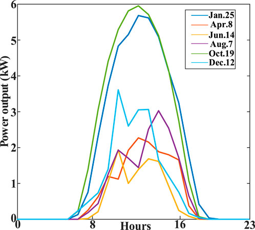
The historical data for the PV power output and meteorological conditions are primarily from the Desert Knowledge Australia Solar Center (DKASC), Alice Springs (latitude 42.18°N and longitude 122.70°E). However, only the cloud datasets are obtained from the Climate Data Store (CDS). The PV power curves exhibit numerous peaks and valleys due to sudden changes in weather conditions. Some example curves are shown in Figure 1.

Figure 1

Figure 1. Curves of PV power in different weather conditions in 1 year.

Therefore, a weather distribution analysis is adopted in this paper to reduce the nonlinearity of meteorological data and mitigate its impact on the prediction model. Additionally, based on weather clustering, the weather variability analysis is included to further investigate the impact of weather, especially cloud changes.

3.1 Weather condition classification

Three indicators include clear sky index (K), total cloud cover (TCC), and diffuse horizontal irradiance fraction (F). TCC describes a proportion of a grid box covered by cloud, which ranges from [0 to1].

K is an index that eliminates the seasonal and daily tendency in time-series data, which is defined as Equation 5:

$K=\frac{GH{I}_{\mathrm{m}}}{GH{I}_{\text{cs}}},(5)$

where GHI_m is the measured global horizontal irradiance and GHI_cs is the hourly irradiance in the clear sky model for a specific area and time.

The weather conditions from the view of irradiance are distinguished by the diffuse horizontal irradiance fraction, which is calculated by the ratio of diffuse horizontal irradiance (DHI) and GHI as Equation 6:

$F=\frac{DHI}{GHI}.(6)$

The detailed calculation process of the clear sky index and the diffuse horizontal irradiance fraction are cited in Rizwan et al. (2021) and Liu et al. (2021).

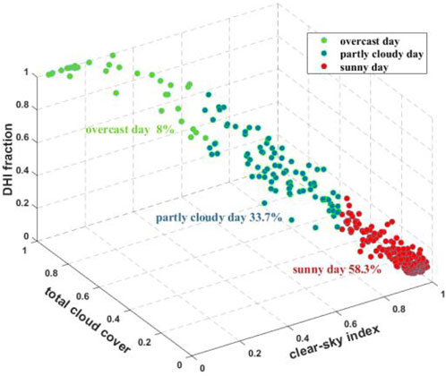
The irradiance data within the time range of the power acquisition (from 6. a.m to 6. p.m) are used to meet the actual power collection situations and facilitate data usage. The irradiance datasets outside of the time range are zero. The datasets are classified into three kinds of weather conditions according to the analysis of weather distribution, namely, sunny day, partly cloudy day, and overcast day, as reported in Table 1. In addition, the corresponding data categories under different weather conditions are shown in Figure 2. The sunny day, partly cloudy day, and overcast day account for 58.3%, 33.7%, and 8% of datasets, respectively.

Table 1

Table 1. Ranges of three kinds of weather conditions under three indicators.

Figure 2

Figure 2. Result of weather condition category.

3.2 Weather variability analysis

Two parameters used in the weather variability analysis are the mean clear sky index in 1 day $\overline{K}$ and the variability index obtained by the standard deviation of the change in the clear sky index V(ΔK).

The daily mean clear sky index characterizes the daily solar radiation in the considered area, which is defined as Equation 7:

$\overline{K}=\frac{{\displaystyle \sum _{T=1}^H}K\left(T\right)}{H},(7)$

where H means the number of daytime hours; in this paper, the daytime hours are the time range of power collection.

The variability index, namely, the nominal variability, indicates the variability of the clear sky index, which is calculated as Equation 8:

$V\left(\Delta K\right)=\sqrt{\frac{{\displaystyle \sum _{T=1}^{H-1}}\left(\Delta K\left(T\right)-\overline{\Delta K}\right)}{H-1}},(8)$

where $\overline{\Delta K}$ is the difference of K during its average value and ΔK(T) is the difference of K during ΔT, as Equation 9:

$\Delta K\left(T\right)=K\left(T+1\right)-K\left(T\right).(9)$

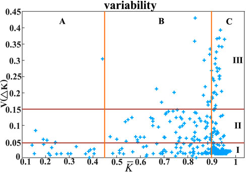
The weather variability is illustrated in Figure 3 based on the clear sky index and the variability index. The variability is divided into two aspects, namely, cloud coverage and variability magnitude, to describe the changes better.

Figure 3

Figure 3. Weather variability of datasets and analyzed using two parameters.

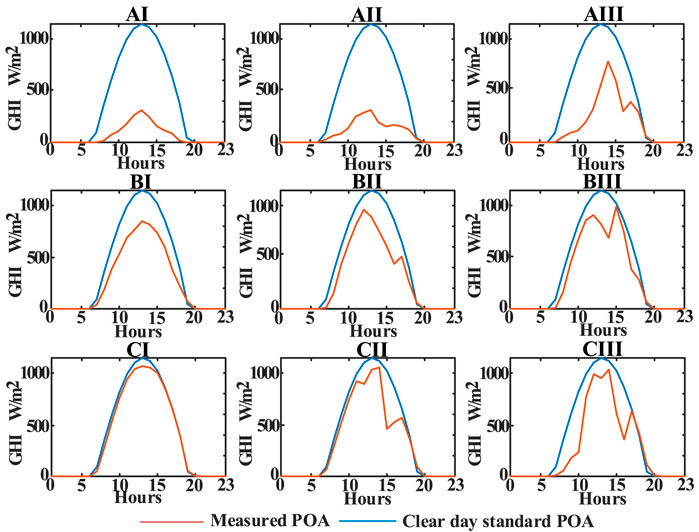
The days are classified into nine blocks, as presented in Figure 4. The mean daily clear sky index is divided into A, B, and C days, where A means heavily cloudy days $\left(0<\overline{K}\le 0.45\right)$, B is partly cloudy days $\left(0.45<\overline{K}<0.9\right)$, and C is the clear cloudy days $\left(0.9\le \overline{K}\le 1\right)$. In the same way, the Roman numbers I, II, and III are used to classify the variability index, where I denotes the slightly variable days (0 < V(ΔK) ≤ 0.05), II is variable days (0.15 ≤ V(ΔK) ≤ 0.45), and III stands for terribly variable days (0.15 ≤ V(ΔK) ≤ 0.45).

Figure 4

Figure 4. Example days of each classification block.

The example day for each block is shown in Figure 4, and the classification results in 1 year are presented in Table 2. According to Table 2, although half of the days were taken up by sunny days in Alice Springs in 1 year, the difficulty of power prediction in cloudy weather increases a lot, and over 30% of weather conditions are high in variability.

Table 2

Table 2. Days of weather variability classification in 1 year.

4 Forecasting model

In the POA irradiation forecasting of this work, usual environmental factors such as wind speed and humidity are added to indicate the environmental effects on the forecasting results, and the cloudiness features are added to quantify the influence of clouds on the irradiance. Therefore, the inputs in POA irradiation forecasting are POA irradiance, temperature, wind speed, relative humidity, lower cloud cover (LCC), medium cloud cover (MCC), and high cloud cover (HCC). Indeed, the function used to relate input datasets, and the irradiance is expressed as Equation 10:

$G_{\text{POA}}\left(t+1\right)=f\left(T_{\text{amb}}\left(t\right),W_{\text{speed}}\left(t\right),RH\left(t\right),G_{\text{POA}}\left(t\right),LCC\left(t\right),MCC\left(t\right),UCC\left(t\right)\right),(10)$

where T_amb(t) is the temperature at time t, W_speed(t) is the wind speed at time t, RH(t) is the relative humidity at time t, and LCC(t), MCC(t), and UCC(t) are LCC, MCC, and UCC at time t, respectively.

The training dataset is divided into input vectors and output vectors of N training patterns as Equation 11:

$Q={\left\{\left({\mathrm{x}}_t,{\mathrm{y}}_t\right)\right\}}_t^p,(11)$

where p represents the pattern numbers. The input vector x_t contains POA irradiance data and meteorological data, while the output vector y_t contains POA irradiance at the forecasting time.

In relation to ambient temperature, numerous variables influence temperature levels; however, the impact of these individual variables is relatively minor. Upon closer examination, a significant degree of interdependence and correlation among these variables is observed, which makes accurate prediction particularly challenging. Therefore, a more streamlined approach is proposed, where historical temperature data are directly used as inputs, rather than attempting to forecast ambient temperature.

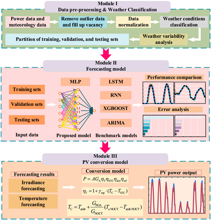
The flow chart of this paper is shown in Figure 5. In Module 1, the pre-processed environmental data, including factors such as temperature, irradiance, and cloud cover, are introduced into the system for weather analysis and classification, where they are categorized based on different weather conditions to enable more accurate modeling. In Module 2, these categorized data are utilized by four benchmark prediction models along with an improved ANN model to predict key environmental variables, which are essential for accurate PV power forecasting. Finally, in Module 3, the predicted environmental variables from Module 2 are input into the PV conversion model, which calculates the PV power output by considering factors such as temperature derating, environmental coefficients, and reflection coefficients, ultimately yielding the final forecast of PV power generation.

Figure 5

Figure 5. Flowing chart of the model.

4.1 ANN forecasting model

The ANN is adopted to find a relation between the input data and output data. The ANN imitates the working mechanism of the human brain, consisting of several individual intelligent units, called neurons, which are used to receive information from the previous neurons or outside and transmit them to the next. Neurons are connected through weights, and linked weights are adjusted to obtain the best weight distribution in the process of training. An activation function is applied to evaluate the output correspondent with the input in each neuron. The activation function is a hyperbolic tangent function in this work, which is calculated as Equation 12:

$f\left(x\right)=\tanh \left(x\right)=\frac{e^{2x}-1}{e^{2x}+1}.(12)$

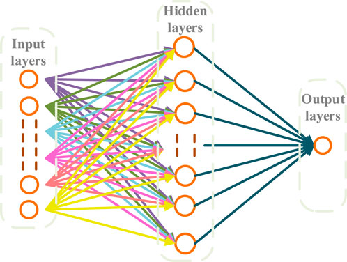
The structure of the ANN is composed of several input layers, one or more hidden layers consisting of neurons, and layers of outputs, which are shown in Figure 6. For the output and input layers, a linear function is used as the activation function, which is given as Equation 13:

$f\left(x\right)=x.(13)$

Figure 6

Figure 6. Structure of the ANN model.

One of the most significant issues that need to be considered is the optimal weight. In this work, the gradient descent method is applied to update weights during the training process. First, a random weight set is chosen as the target set. Then, a cost function, namely, the mean squared error (MSE) cost function, is used to calculate the average of difference between the network output (forecasting value) and the real value. At last, the minimum value of the cost function is obtained by the backpropagation algorithm. The cost function is expressed as Equation 14:

$J\left(w,b\right)=\frac{1}{\mathrm{m}}{\displaystyle \sum _{i=1}^{\mathrm{m}}}{\left(h\left(x_i\right)-y_i\right)}^2,(14)$

where h (x_i) is the network output, y_i represents the real value, w is the weight coefficient, b is the bias coefficient, and m is the number of unknowns.

The model complexity is another significant issue. Over complex ANN structures may lead to poor results due to the problem of overfitting. L2 regularization is proposed to control the complexity and achieve good generalization results. The L2 regularization method considers the sum of squares of weight parameters, which smooths the cost function, and a new hyperparameter λ is introduced to control the error. The smooth cost function reduces the influence when the input is corrupted by the noise in the training process. The optimal complexity corresponds to the minimum of the following new cost function as Equation 15:

$L\left(w,b\right)=\frac{1}{\mathrm{m}}{\displaystyle \sum _{i=1}^{\mathrm{m}}}{\left(h\left(x_i\right)-y_i\right)}^2+\frac{\lambda }{2m}{\displaystyle \sum _{j=1}^m}{w}_j^2.(15)$

In addition, a Gaussian distribution is applied to initialize the weights randomly, in order to decrease the computation of the backpropagation algorithm and improve the computational precision, which is calculated as Equation 16:

$N\left(w|\mu ,{\sigma }^2\right)=\sqrt{\frac{1}{2\pi {\sigma }^2}}{\mathrm{e}}^{-\frac{{\left(x-\mu \right)}^2}{2{\sigma }^2}}.(16)$

An iteration process should be followed to obtain the optimal hyperparameter λ and weight parameter w. At first, the weights are randomly initialized by Gaussian distribution, and the hyperparameter values are in an appropriate range. Then, the first optimized weight sets are obtained by the backpropagation algorithm, which are used in the calculation of the hyperparameter. At last, the hyperparameters are computed by the L2 regularization. These steps are repeated until the sum of squares of weights is less than the critical value C(C = 1).

4.2 ANN model optimization

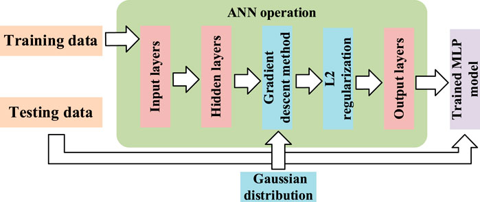
In this paper, the Keras library written by Python is used for building the ANN structure. The improvement of the ANN forecasting results combining irradiance data, temperature data, and other meteorology data as inputs is focused on this paper. The flowing chart of the ANN model is illustrated in Figure 7.

Figure 7

Figure 7. Flowing chart of the ANN model.

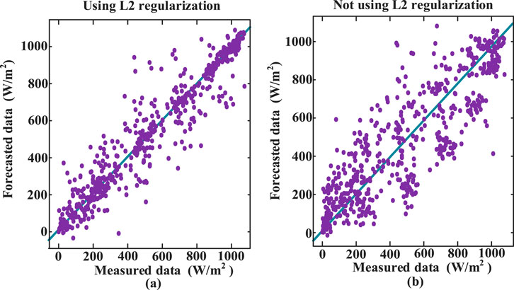
In this paper, ANN model complexity and overfitting are taken into consideration to improve forecasting results. The normal ANN model will undergo overfitting due to the complex structure. Therefore, L2 regularization is used for controlling the complexity and avoiding overfitting. The effect of L2 regularization is shown in Figures 8, 8A, while Figure 8B shows the results without L2 regularization. After applying L2 regularization, the forecasted results align more closely with the measured data.

Figure 8

Figure 8. Effect of L2 regularization,(A) with L2 regularization and (B) without L2 regularization.

5 Case study

Studies and evaluations of the ANN forecasting model are presented in this section. All simulations are realized on a workstation with Intel(R) i7-10875CPU @2.30 GHz, NVIDIA RTX 2070s, and 32 GB RAM memory. This section consists of dataset description, benchmark models, performance evaluation metrics, experimental studies, and results of PV power.

5.1 Dataset description

The PV power historical data collected from the DKASC are used. The data of cloud amount are from the CDS, and other weather data are collected from the meteorological stations surrounded with the DKASC. The time interval of datasets used in this paper is 5 minutes. The length of all data is 1 year, which is from 1st January 2020 to 31st December 2020. The dividing ratio of the training set, validation set, and testing set is set as 0.7:0.1:0.2. In addition, in the process of validation, 10-fold cross-validation is applied in evaluating the training results. The forecasting horizon of this paper is 24 h. In addition, three typical days are selected from each of the three clustering results as the prediction day.

5.2 Benchmark models

A total of four benchmark models are used to compare with the MLP model to evaluate the performance. The four benchmark models are LSTM, ARIMA, SVR, and XGBOOST. The LSTM model has high prediction accuracy, but there may be some prediction bias in case of too much training data. The ARIMA model is suitable for stationary datasets, but its prediction results may be inaccurate when there are many fluctuations. The SVR model belongs to linear regression models and may have lower accuracy than neural networks, but it can better describe data fluctuations. XGBOOST is a commercially available prediction model with high accuracy and can be applied to various scenarios.

5.3 Performance evaluation metrics

Four standard evaluation metrics widely used in the forecasting community are adapted to evaluate the performances of models, including the root mean squared error (RMSE), normalized RMSE (nRMSE), mean absolute error (MAE), and normalized MAE (nMAE). In addition, the forecasting skill parameter is calculated to compare the improvement of different models with the persistence model. These metrics are defined as Equations 17–20:

$\text{RMSE}=\sqrt{\frac{1}{N}{\displaystyle \sum _{t=1}^N}{\left({\widehat{Y}}_t-Y_t\right)}^2},(17)$

$\text{nRMSE}=\frac{\sqrt{\frac{1}{N}{\displaystyle \sum _{t=1}^N}{\left({\widehat{Y}}_t-Y_t\right)}^2}}{Y_a}\times 100\%,(18)$

$\text{MAE}=\frac{1}{N}{\displaystyle \sum _{t=1}^N}\left|{\widehat{Y}}_t-Y_t\right|,(19)$

$\text{nMAE}=\frac{\frac{1}{N}{\displaystyle \sum _{t=1}^N}\left|{\widehat{Y}}_t-Y_t\right|}{Y_a}\times 100\%,(20)$

where ${\widehat{Y}}_t$ and Y_t are the forecasted and measured values at time t, respectively, and Ya is the average of the measured values. The performance of the proposed models is dependent on the decrease in RMSE, nRMSE, MAE, and nMAE.

5.4 Outage probability

5.4.1 Sunny day forecasting

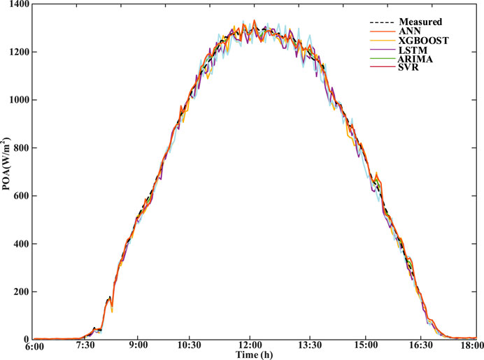
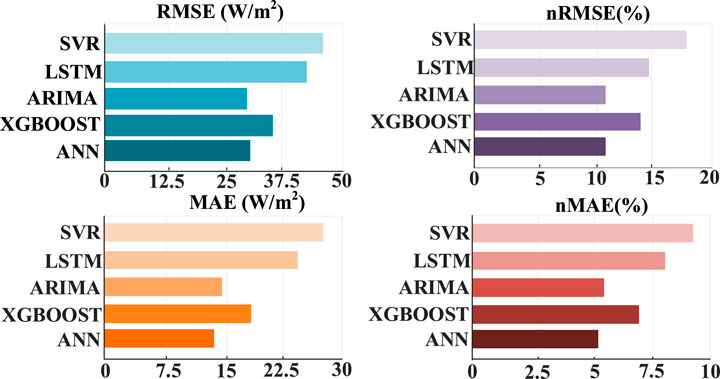
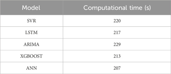
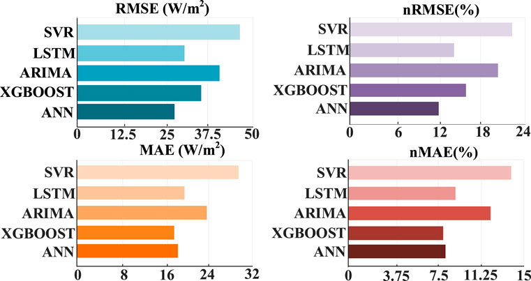
The irradiance prediction results on a sunny day are shown in Figure 9. Under sunny weather, not only the ANN model proposed in this paper has accurate prediction values but also the four benchmark prediction models have better results. As shown in Figure 10, the evaluation indexes of each prediction model show that RMSE and nRMSE of ARIMA are superior to those of other models on sunny days. The computational time of each model is shown in Table 3. The ANN model proposed in this paper is superior to the four benchmark models in MAE and nMAE and is almost the same as ARIMA in RMSE and nRMSE. The RMSE of ANN is 2.34%, which is higher than that of ARIMA, but the computational time is 2.87%, which is better than that of ARIMA, indicating that the proposed method has a good prediction effect in the case of flat curves. The SVR has the worst prediction result because the linear regression model faces difficulty in describing the complex nonlinear mapping relationship, so its prediction effect is worse than that of the neural network and other models.

Figure 9

Figure 9. Forecasting results of irradiance on the sunny day.

Figure 10

Figure 10. Performance metrics of irradiance forecasting for each model on sunny day.

Table 3

Table 3. Computational time of each model on the sunny day.

5.4.2 Partly cloudy day forecasting

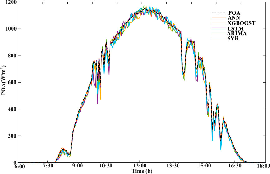
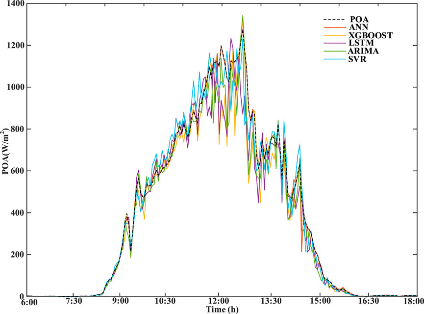
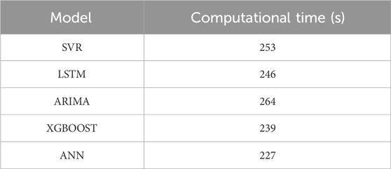
In cloudy weather, cloud formation and subsequent cloud movement can cause fluctuations in irradiance and also increase the difficulty in prediction. The irradiance prediction results under cloudy weather are shown in Figure 11. It can be seen from the figure that several of them can better capture the fluctuations. The computational time of each model is shown in Table 4. The evaluation indexes of different prediction models are shown in Figure 12. In terms of RMSE and nRMSE evaluation indicators, the results of the proposed ANN model are better than those in other models, which are 25.4% and 25% lower than XGBOOST, respectively. However, in terms of MAE and nMAE, the results of XGBOOST are better than those of the proposed ANN model, which are 5.56% and 4.97%, respectively. This is because XGBOOST can traverse all the eigenvalues in the data information to increase the information gain, so it has better prediction results in such scenarios with partial fluctuations, but this will increase the computation and training time. The proposed ANN model has a small gap with XGBOOST in terms of indicators, but the training time is 3%, which is better than that of XGBOOST. Therefore, the comprehensive prediction result of the ANN is better than that of XGBOOST.

Figure 11

Figure 11. Forecasting results of irradiance on the partly cloudy day.

Table 4

Table 4. Computational time of each model on partly cloudy day.

Figure 12

Figure 12. Performance metrics of irradiance forecasting for each model on the partly cloudy day.

5.4.3 Overcast day forecasting

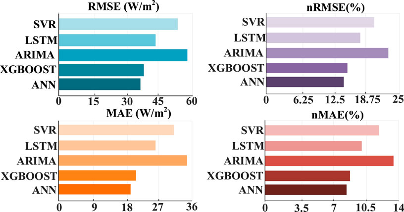
On overcast days, the sky is obscured by various clouds, which have a strong blocking effect on solar radiation, so there will be a lot of fluctuations. The irradiance predicted values of each forecasting model under cloudy skies are shown in Figure 13. The computational time of each model is shown in Table 5. Figure 14 shows the performance indicators of different models in irradiance prediction. As can be seen from the figure, the evaluation indexes of the ANN model proposed are superior to those of the other four models, which are 3.31% lower than that XGBOOST on RMSE and 2.87% lower than XGBOOS on MAE. The reason for the worst performance of ARIMA is that ARIMA is only applicable to curves with a relatively stable wave shape, and there are a lot of fluctuations in the data. This method cannot capture a lot of fluctuation characteristics, indicating that it will have poor prediction effects on cloudy days with large fluctuations.

Figure 13

Figure 13. Forecasting results of irradiance on the overcast day.

Table 5

Table 5. Computational time of each model on partly cloudy day.

Figure 14

Figure 14. Performance metrics of irradiance forecasting for each model on overcast day.

5.4.4 Results of the PV power output

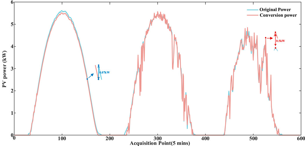
The predicted POA irradiance and ambient temperature are inputted into the photoelectric conversion model, and the photovoltaic power obtained through the photoelectric conversion model is shown in Figure 15. The loss refers to the difference between these two power values. The maximum loss point is 0.5 kW, which is enlarged and shown in red in the figure. The minimum loss is 0.07 kW, which is enlarged and shown in blue in the figure. The average error is 0.16 kW, and the error loss is within the acceptable range. Compared with the measured power, the error rate is 3.3% in sunny days, 4.5% in cloudy days, and 5.2% in partly cloudy days. Through the hybrid prediction model, the prediction error and physical error in the prediction can be intuitively seen to achieve the effect of error separation, and the photovoltaic power obtained by this is more real.

Figure 15

Figure 15. Photoelectric conversion model results.

6 Conclusion

An accurate short-term forecasting method plays a significant role in enhancing power grid dispatch. This paper proposes a hybrid forecasting model to improve the accuracy of short-term PV power forecasts under various weather conditions.

1) The photovoltaic power obtained by the proposed hybrid model differs by 4.3% from the true value and is approximately 2% more accurate than directly predicting photovoltaic power, meeting practical requirements. The PV .power obtained by the proposed hybrid model is closer to true values and meets actual demands due to the accurate forecasting results by the ANN model and the PV conversion model.

2) The ANN network improved by L2 regularization, and gradient descent reduced the error of irradiance prediction by approximately 6%. On sunny day, partly cloudy day, and overcast day forecasting, the improved MLP model can perform better than other benchmark models. The proposed ANN model has shown good prediction results in all three weather models, with an overall evaluation index of approximately 15% higher than other models and a calculation time reduction of approximately 8% compared to other models.

3) Cloud amount plays a significant role in the process of irradiance forecasting. The addition of cloud amount to irradiance forecasting can obviously influence the forecasting accuracy, especially on cloudy and variable days.

4) Weather classification can divide the forecasting scenarios and improve the quality of the PV generation under different weather conditions. Weather variability analysis further classifies different variable days and provides a basis for the increased prediction accuracy of PV power in various meteorological conditions.

Data availability statement

The original contributions presented in the study are included in the article/supplementary materials, further inquiries can be directed to the corresponding author/s.

Author contributions

RC: writing–review and editing. SG: writing–original draft. YZ: writing–review and editing. DL: writing–review and editing. SL: writing–review and editing.

Funding

The author(s) declare that financial support was received for the research, authorship, and/or publication of this article. This study was funded by the Shanghai Rising-Star Program (No. 21QC1400200), Natural Science Foundation of Shanghai (No. 21ZR1425400), and National Natural Science Foundation of China (No. 52377111).

Conflict of interest

Author RC was employed by State Grid Shanghai Electric Power Company. Author SG was employed by State Grid Shanghai Electric Power Company Qingpu Power Supply Company.

The remaining authors declare that the research was conducted in the absence of any commercial or financial relationships that could be construed as a potential conflict of interest.

Publisher’s note

All claims expressed in this article are solely those of the authors and do not necessarily represent those of their affiliated organizations, or those of the publisher, the editors, and the reviewers. Any product that may be evaluated in this article, or claim that may be made by its manufacturer, is not guaranteed or endorsed by the publisher.

References

Barbieri, F., Rajakaruna, S., and Ghosh, A. (2017). Very short-term photovoltaic power forecasting with cloud modeling: a Review. Renew. Sust. Ener Rev. 75, 242–263. doi:10.1016/j.rser.2016.10.068

CrossRef Full Text | Google Scholar

Bishop, C. M. (1995). Neural networks for pattern recognition. New York, USA: Oxford University Press, 116–137.

CrossRef Full Text | Google Scholar

Bouzerdoum, M., Mellit, A., and Pavan, A. M. (2013). A hybrid model (SARIMA–SVM) for short-term power forecasting of a small-scale grid-connected photovoltaic plant. Sol. energy 98, 226–235. doi:10.1016/j.solener.2013.10.002

CrossRef Full Text | Google Scholar

De la Parra, I., Muñoz, M., Lorenzo, E., García, M., Marcos, J., and Martínez-Moreno, F. (2017). PV performance modelling: a review in the light of quality assurance for large PV plants. Renew. Sust. Ener Rev. 78, 780–797. doi:10.1016/j.rser.2017.04.080

CrossRef Full Text | Google Scholar

Diagne, M., David, M., Lauret, P., Boland, J., and Schmutz, N. (2009). Review of solar irradiance forecasting methods and a proposition for small-scale insular grids. Renew. Sust. Ener Rev. 27, 65–76. doi:10.1016/j.rser.2013.06.042

CrossRef Full Text | Google Scholar

Gao, M., Li, J., Hong, F., and Long, D. (2019). Day-ahead power forecasting in a large-scale photovoltaic plant based on weather classification using LSTM. Energy 187, 115838. doi:10.1016/j.energy.2019.07.168

CrossRef Full Text | Google Scholar

Ge, L., Xian, Y., Yan, J., Wang, B., and Wang, Z. (2020). A hybrid model for short-term PV output forecasting based on PCA-GWO-GRNN. J. Mod. Power Syst. Cle. 8 (6), 1268–1275. doi:10.35833/mpce.2020.000004

CrossRef Full Text | Google Scholar

Liu, L., Zhao, Y., Chang, D., Xie, J., Ma, Z., Sun, Q., et al. (2021). Prediction of short-term PV power output and uncertainty analysis. Appl. energy 228, 700–711. doi:10.1016/j.apenergy.2018.06.112

CrossRef Full Text | Google Scholar

Ma, Y., Lv, Q., Zhang, R., Zhang, Y., Zhu, H., and Yin, W. (2021). Short-term photovoltaic power forecasting method based on irradiance correction and error forecasting. Energy Rep. 7, 5495–5509. doi:10.1016/j.egyr.2021.08.167

CrossRef Full Text | Google Scholar

Martins, F. R., Pereira, E. B., and Guarnieri, R. A. (2012). Solar radiation forecast using artificial neural networks. Inter J. Ener Scien 2 (5), 217–227. doi:10.5772/intechopen.70570

CrossRef Full Text | Google Scholar

Mellit, A., and Pavan, A. M. (2010). A 24-h forecast of solar irradiance using artificial neural network: application for performance prediction of a grid-connected PV plant at Trieste, Italy. Sol. energy 84 (5), 807–821. doi:10.1016/j.solener.2010.02.006

CrossRef Full Text | Google Scholar

Mustafa, R. J., Gomaa, M. R., Al-Dhaifallah, M., and Rezk, H. (2020). Environmental impacts on the performance of solar photovoltaic systems. Sustainability 12 (2), 608–624. doi:10.3390/su12020608

CrossRef Full Text | Google Scholar

Rizwan, M., Jamil, M., Kirmani, S., and Kothari, D. (2021). Fuzzy logic based modeling and estimation of global solar energy using meteorological parameters. Energy 70, 685–691. doi:10.1016/j.energy.2014.04.057

CrossRef Full Text | Google Scholar

Tascikaraoglu, A., Sanandaj, B. M., Chicco, G., Cocina, V., Spertino, F., Erdinc, O., et al. (2016). Compressive spatio-temporal forecasting of meteorological quantities and photovoltaic power. IEEE Trans. Sustain. Energy 7 (5), 1295–1305. doi:10.1109/TSTE.2016.2544929

CrossRef Full Text | Google Scholar

Torres-Ramírez, M., Nofuentes, G., Silva, J. P., Silvestre, S., and Muñoz, J. (2014). Study on analytical modelling approaches to the performance of thin film PV modules in sunny inland climates. Energy 7, 731–740. doi:10.1016/j.energy.2014.06.077

CrossRef Full Text | Google Scholar

Visser, L., AlSkaif, T., and van Sark, W. (2022). Operational day-ahead solar power forecasting for aggregated PV systems with a varying spatial distribution. Renew. Energ 183, 267–282. doi:10.1016/j.renene.2021.10.102

CrossRef Full Text | Google Scholar

Wang, F., Xuan, Z., Zhen, Z., Li, K., Wang, T., and Shi, M. (2019). A day-ahead PV power forecasting method based on LSTM-RNN model and time correlation modification under partial daily pattern prediction framework. Energ Convers. Manage 212, 112766. doi:10.1016/j.enconman.2020.112766

CrossRef Full Text | Google Scholar

Wang, M., Peng, J., Luo, Y., Shen, Z., and Yang, H. (2021). Comparison of different simplistic prediction models for forecasting PV power output: assessment with experimental measurements. Energy 224, 120162. doi:10.1016/j.energy.2021.120162

CrossRef Full Text | Google Scholar

Wolff, B., Kühnert, J., Lorenz, E., Kramer, O., and Heinemann, D. (2020). Comparing support vector regression for PV power forecasting to a physical modeling approach using measurement, numerical weather prediction, and cloud motion data. Sol. energy 135, 197–208. doi:10.1016/j.solener.2016.05.051

CrossRef Full Text | Google Scholar

Zhao, Y., Gao, S., and Li, D. (2023). Short-term interval probability prediction of photovoltaic power based on weather similarity clustering and quantile regression neural network. Automation Electr. Power Syst. 47:152–161. doi:10.1109/iciea58696.2023.10241566

CrossRef Full Text | Google Scholar