Research on urban power load forecasting based on improved LSTM

In this paper, the maximal information coefficient method-variational mode decomposition-bidirectional long short term memory network-adaptive boosting (MIC-VMD-Bi-LSTM-Adaboost) algorithm is used to forecast the power load. Firstly, MIC is used to determine the correlation degree of meteorological parameters influencing power load. Features having a high correlation degree are then chosen to be input vectors. Secondly, the input characteristics are decomposed using VMD, and five distinct IMF components are retrieved in order to remove unnecessary information. Lastly, different assessment indices are computed and the power load is predicted using the Bi-LSTM-Adaboost method. In order to determine the benefit of the approach used in this work, the outcomes of LSTM, Bi-LSTM, and LSTM-Adaboost are compared concurrently.

1 Introduction

Power load forecasting is a key step in power industry planning. It comprehensively predicts and calculates future power load, power consumption situation, power demand and power consumption based on historical power load data and other relevant interfering factors (such as weather changes, human activities, industrial process types, time and seasonal characteristics, etc.) (Habbak et al., 2023). Accurate forecast and rapid response to power demand are critical to the safety, stability and efficiency of power system operation (Kumar, 2024). Electric vehicles, renewable energy, flexible loads and other unpredictable loads are being added to the modern power grid. It also enhances the accuracy of load forecasting (Kumar et al., 2013).

Existing load prediction approaches can be categorized into two types: conventional mathematical statistics and machine learning (Chen et al., 2023). Traditional mathematical statistics approaches include regression analysis, kalman filtering, load derivation, and exponential smoothing (Kumar et al., 2016). These approaches are basic in structure, operate and forecast quickly, and may be scaled. However, they rely on statistical law characteristics, and the results of nonlinear data processing are poor, with low precision (Kumar et al., 2020).

Machine learning methods for load forecasting, including neural network (NN), support vector machine (SVM), and long short term memory network (LSTM), have been developed with advancements in computer technology (Cordeiro-Costas et al., 2023). These strategies improve prediction accuracy and overcome the limitations of nonlinear data (Kumar et al., 2023b). In the actual prediction process, two or more algorithms are generally used to complement each other, and other meteorological factors are included, to make the forecast findings more realistic (Kumar et al., 2023a).

Currently, researchers have employed a combination of multiple techniques to anticipate load. Tian et al. (2022) Neural networks (NN) were integrated with type-2 fuzzy systems (T2FSs), and feedback was introduced to the fuzzy neural networks. This approach achieved an accuracy of 98$\%$. Rafi et al. (2021) used a combination of CNN and LSTM to anticipate power load in the short term. It outperforms LSTM, RBFNN, and XGBoost in terms of prediction accuracy. Compared with the prediction of LSTM, radial basis function neural network (RBFNN) and extreme gradient boosting (XGBoost), it has higher accuracy. Guo et al. (2022) proposed a MES load prediction algorithm according to multi-task learning of Bi-LSTM, analyzed the relevance of load in four seasons, and selected different load combinations with MIC as input vectors to realize the associated information sharing between loads. Bareth et al. (2024) used LSTM to predict the average daily load demand per month in 2023 based on the average daily load demand per day, considering the average daily load demand per month from 2018 to 2022. The results show that the LSTM network is more appropriative for real-time load demand forecasting. Aguilar Madrid and Antonio (2021) used XGBoost algorithm to predict power load. Compared with multiple linear regression (MLR), k-nearest neighbor regression (KNN), epsilon-support vector regression (e-SVR) and random forest regression (RF), it shows that the algorithm has stronger performance. Álvarez et al. (2021) proposed a logical load prediction approach according to adaptable online learning of hidden Markov model, developed adaptable online learning technology, and recursively updated model parameters. In Deng et al. (2021), a short-term load prediction model according to enhanced genetic expression mechanism and abnormal load identification is proposed. The abnormal load identification algorithm according to degree distribution and cross-verification solves the problem of misjudgment of normal values. By designing the adaptive evolution strategy of population variables, the individual evolution strategy of population and the dynamic modification strategy of genetic performance probability, a modified gene expression planning approach according to evolutionary parameter improvement is presented. The algorithm is superior to other algorithms in misdetection rate, error detection rate and accuracy. Moreira-Júnior et al. (2022) used Fuzzy-ARTMAP neural network to predict substation load, to enhance the precision of multi-node load prediction. In Deng et al. (2022), a quantitative combined load prediction model (QCLF) is presented. The improved k-means algorithm is combined with the least squares algorithm to boost the reliability of the data, and the gene expression programming optimization is used. Wan et al. (2023) proposed CNN-LSTM-Attention to improve the accuracy of load forecasting. Pearson correlation coefficient analyzes the main factors affecting load. Attention mechanism optimizes LSTM output weight and enhances key information. Nie et al. (2020) proposed the radial basis function-generalized regression neural network-extreme learning machine (RBF-GRNN-ELM) fusion algorithm, which considers data preprocessing, individual prediction algorithm and weight determination theory, and improves the prediction accuracy. In Ge et al. (2020), the power load is predicted by the combination of improved k-means clustering, reinforcement learning, particle swarm optimization and least squares support vector machine. Wu et al. (2020) proposed a fusion algorithm of autoregressive integrated moving average (FARIMA) and cuckoo search algorithm (CSA), and the prediction effect is perfect. In Du et al. (2020), an optimization technique for predicting power load is proposed using Bi-LSTM-Attention fusion. Compared to other algorithms, the algorithm is more robust.

The above literature uses MIC, LSTM and XGBoost algorithms for load forecasting, but does not combine the algorithms, and does not consider the impact of various feature vectors on load forecasting. Considering the large amount of data, the direct prediction calculation is large and the data is redundant, which will also reduce the prediction accuracy. Therefore, a VMD of various meteorological factors affecting power load is proposed in this paper, and the Bi-LSTM combined with Adaboost algorithm is used to predict power load. Firstly, MIC is used to analyze the relevance of input factors affecting prediction, and the features with high correlation coefficient are extracted as input. Secondly, the input factors are decomposed by VMD to eliminate noise and avoid redundant data. Finally, Bi-LSTM combined with Adaboost algorithm is used to predict urban power load, and root mean square error (RMSE), mean absolute error (MAE), mean absolute percentage error (MAPE) and coefficient of determination ($R^2$) are used as evaluation indexes to judge the prediction results, which are compared with the forecasting outcome of LSTM, Bi-LSTM and LSTM-Adaboost respectively, so as to highlight the superiority of this method. At the same time, the calculation amount of this method is small, the prediction time is short, and it is feasible for the situation with high time requirement.

2 Feature processing

2.1 Maximal information coefficient method

The MIC is used to assess the extent of significance between variables, linear or nonlinear strength, and is frequently employed in feature selection. It has good universality, fairness, and symmetry (Lin et al., 2022). Table 1 presents a comparison of commonly used methods. It can be seen that MIC has minimal computing complexity, great stability, and apparent advantages.

Table 1

Table 1. Comparison of various algorithms.

The theory of MIC is according to the concept of mutual information. Mutual information refers to the measure of interdependence between variables, that is, the degree of uncertainty reduction of random variable X to Y, which is expressed by Equation 1. The larger the value, the stronger the correlation between the two variables; conversely, the weaker the correlation. When I (X; Y) = 0, X and Y are independent.

$I\left(X;Y\right)=\underset{Y}{\int }\underset{X}{\int }p\left(x,y\right){\log }_2\frac{p\left(x,y\right)}{p\left(x\right)p\left(y\right)}dxdy(1)$

Here, $I(X;Y)$ is the mutual information measure of two random variables. $x$ and $y$ are two vectors, $p(x,y)$ is the joint probability density of vector $x$ and $y$, $p(x)$ and $p(y)$ are the marginal probability density of vector $x$ and $y$, respectively.

The idea of MIC is as follows: according to the relationship between the two variables, the scatter plot is used to distribute in the two-dimensional space, and a certain interval is divided in the x and y directions respectively, and the distribution of all scatters in each interval is checked (Surapunt and Wang, 2024). Formula 2 is the calculation of MIC.

$MIC\left(x,y\right)=\underset{a^{*}b<B}{\max }\frac{I\left(x,y\right)}{{\log }_2\min \left(a,b\right)}(2)$

In the formula, $a$ and $b$ are the number of intervals divided horizontally and vertically respectively, and $B$ is a variable, which is approximately 0.6 power of the total data.

According to Equations 1, 2, MIC can be divided into three steps:

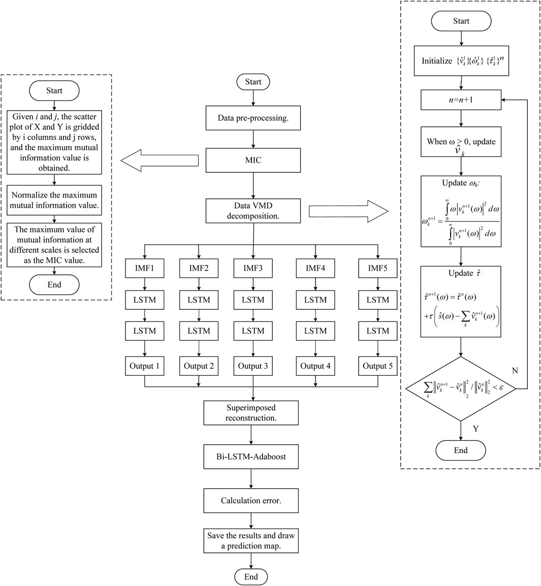
1. Given i and j, the scatter plot composed of XY is gridded by i columns and j rows, and the maximum mutual information value is obtained;

2. Normalize the maximum mutual information value;

3. The maximum value of mutual information at different scales is selected as the MIC value.

2.2 Feature extraction

MIC analyzes the degree of correlation between each feature and the load size since it is uncertain how much each affecting factor will effect the load (Sukanya Satapathy and Kumar, 2020; Satapathy and Kumar, 2019). The correlation is higher the greater the value’s absolute value. The correlation degree corresponding to various correlation coefficients is displayed in Table 2.

Table 2

Table 2. Correlation.

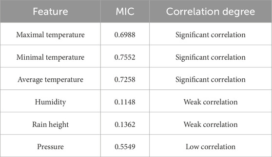
The correlation between the seven meteorological factors affecting the power load and the power value are obtained by MIC, and the outcomes are presented in Table 3.

Table 3

Table 3. MIC correlation analysis.

Table 3 shows significant correlations between highest temperature, lowest temperature, average temperature, and power load. However, humidity, rain height, and pressure show weak and low correlations, which can be ignored. Therefore, the first three are used as inputs.

2.3 VMD decomposition

VMD enables the simultaneous extraction of decomposition modes. The model looks for a group of modes and their respective center frequencies so that they can replay the input signal together, and each mode is smooth after demodulation to the baseband. The algorithm’s essence is to expand the conventional Wiener filter to multiple adaptive bands, giving it a solid theoretical foundation while remaining simple to understand. The alternate direction multiplier method is utilized to successfully improve the variational model, increasing its robustness to sampling noise. The adaptability of VMD refers to the effective decomposition of intrinsic mode function (IMF) components and frequency domain section of signals by adaptively matching the optimal central frequency and bandwidth of every pattern while performing pattern decomposition on a given sequence, in order to obtain effective signal decomposition components and get the suitable results of the variational problem (Zhao et al., 2023; Wang et al., 2023). The following Equations 3–6 are the solution formulas of VMD decomposition (Geng et al., 2023). The VMD decomposition of highest temperature, lowest temperature and average temperature is shown in (Figures 1A–C).

$\left[\left(\delta \left(t\right)+\frac{\left.j\right)}{\pi t}\right)v_k\left(t\right)\right]e^{-j{\omega }_{k}t}(3)$

$\min \left\{{\displaystyle \sum _k}{‖{\partial }_t\left[\left(\delta \left(t\right)+\frac{j}{\pi t}\right)v_k\left(t\right)\right]e^{-j{\omega }_{k}t}‖}^2\right\}.(4)$

$\begin{array}{cc}\hfill L\left(\left\{v_k\right\},\left\{{\omega }_k\right\},\tau \right)& =\alpha {\displaystyle \sum _k}{‖{\partial }_t\left[\left(\delta \left(t\right)+\frac{j}{\pi t}\right)v_k\left(t\right)\right]e^{-j{\omega }_{k}t}‖}^2+\mid s\left(t\right)-{\displaystyle \sum _k}{v}_k\left(t\right){\Vert }^2\hfill \\ \hfill & +⟨\tau \left(t\right),s\left(t\right)-{\displaystyle \sum _k}{v}_k\left(t\right)⟩\hfill \end{array}(5)$

${\widehat{v}}_k^{n+1}\left(\omega \right)=\frac{\widehat{s}\left(\omega \right)-\sum {\widehat{v}}_i\left(\omega \right)+\widehat{\tau }\left(\omega \right)/2}{1+2\alpha {\left(\omega -{\omega }_k\right)}^2}(6)$

In these formulas, $\delta (t)$ is Dirac function and * is convolution operation. $v_k(t)$ is the analysis signal after Hilbert transform. $\left\{v_k\right\}=\left\{v_1,\dots ,v_k\right\}$ is the decomposed IMF component, and $\left\{{\omega }_k\right\}=\left\{{\omega }_1,\dots ,{\omega }_k\right\}$ is the center frequency of every component part. $\tau (t)$ is the Lagrange multiplier and $\alpha$ is the second-order penalty factor, so as to reduce the interference of Gaussian noise. $\omega$ is the frequency and ${\widehat{v}}_k^{n+1}(\omega )$, $\widehat{s}(\omega )$, $\widehat{\tau }(\omega )$is the Fourier transformation of $v_k^n(t)$, $s(t)$, $\tau (t)$, respectively.

3 Forecasting model

3.1 LSTM network

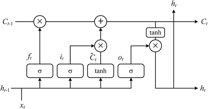
As a peculiar recurrent neural network, LSTM is primarily applied to predict time series (Abumohsen et al., 2023). The Figure 2 is a typical LSTM structure diagram. Bi-LSTM is an improved version of LSTM. The prediction process mainly includes three stages: forgetting stage, selective memory stage and output stage.

Figure 1

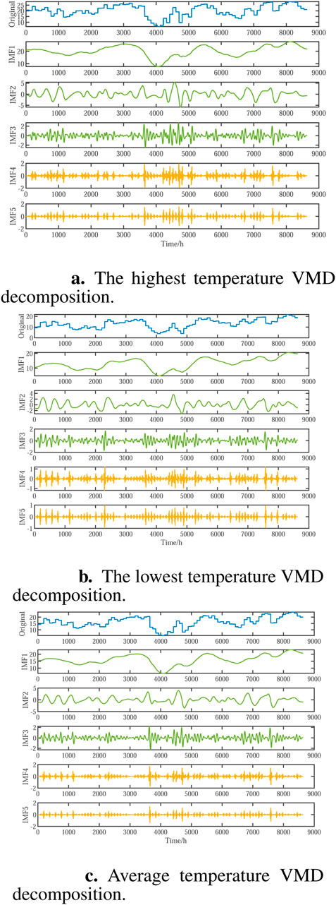
Figure 1. Feature decomposition. (A) The highest temperature VMD decomposition. (B) The lowest temperature VMD decomposition. (C) Average temperature VMD decomposition.

Figure 2

Figure 2. LSTM structure diagram.

The following Formula 7–11 is the calculation of LSTM network (Madhukumar et al., 2022; Jailani et al., 2023).

$f^{\left(t\right)}=\sigma \left(W_f{h}^{\left(t-1\right)}+W_f{x}^{\left(t\right)}+b_f\right)(7)$

$\begin{array}{c}\hfill i^{\left(t\right)}=\sigma \left(W_i{h}^{\left(t-1\right)}+W_i{x}^{\left(t\right)}+b_i\right)\hfill \\ \hfill c^{\left(t\right)}=\tanh \left(W_c{h}^{\left(t-1\right)}+W_c{x}^{\left(t\right)}+b_c\right)\hfill \end{array}(8)$

$C^{\left(t\right)}=C^{\left(t-1\right)}\cdot f^{\left(t\right)}+i^{\left(t\right)}\cdot c^{\prime \left(t\right)}(9)$

$\begin{array}{c}\hfill o^{\left(t\right)}=\sigma \left(W_0{h}^{\left(t-1\right)}+W_0{x}^{\left(t\right)}+b_0\right)\hfill \\ \hfill h^{\left(t\right)}=o^{\left(t\right)}\tanh \left(C^{\left(t\right)}\right)\hfill \end{array}(10)$

${\tilde{y}}^{\left(t\right)}=\sigma \left(V{h}^{\left(t\right)}+c\right)(11)$

Among them, $\sigma$ is the sigmoid activation function, $b_f$ is the forgetting gate boundary, and $W_f$ is the forgetting gate weight. $W_i$, $W_c$ are the weights and $b_i$, $b_c$ are the boundaries of the input gate, respectively. $W_0$ is the weights and $b_0$ is the boundary according to the output gate, respectively, and $h^{(t)}$ is the output vector in the hidden layer. $V$ and $c$ are the weights and boundaries linking the hidden layer to the output layer, respectively.

3.2 Adaboost algorithm

Boost is also known as reinforcement learning, which is an important ensemble learning strategy. It can help weak learners become strong learners with excellent predicting accuracy (Huang et al., 2022). The Adaboost (adaptive boosting) algorithm is self-adaptive in that it increases the weight of samples incorrectly classified by the prior fundamental classifier while decreasing the weight of correctly classified samples, which are reused for training the next basic classifier (Park and Son, 2023). Meanwhile, in each iteration, a new weak classifier is added when a low enough error rate or a certain maximum number of iterations is reached, confirming the final strong classification.

3.3 MIC-VMD-Bi-LSTM-Adaboost model

In this study, the MIC-VMD-Bi-LSTM-Adaboost fusion algorithm is applied to forecast urban power demand. To begin, MIC is used to calculate the correlation degree of each meteorological element to power load, and the meteorological parameters with a high correlation degree are selected as input. Second, the VMD technique is used to breakdown the input object, removing superfluous data and improving accuracy. Finally, the Bi-LSTM fusion Adaboost solver is utilized to perform the final predicting, and the results are produced. Figure 3 depicts the prediction flow chart.

Figure 3

Figure 3. Prediction flow chart.

4 Example analysis

4.1 Data pre-processing

Firstly, the data is cleaned, that is, the wrong data and missing data are eliminated; then, the data is normalized to make the data in the same order of magnitude, which is also used in the subsequent prediction. The normalized calculation formula is shown in Equation 12:

$x^{,}=\frac{x-x_{\min }}{x_{\max }-x_{\min }}(12)$

In the formula, x^, is the processed data, $x$ is the raw data, $x_{\mathit{min}}$ and $x_{\mathit{max}}$ are the minimum and maximum values under a certain feature respectively.

After the prediction, the normalized data is denormalized, as shown in Equation 13.

$x=x\left(x_{\max }-x_{\min }\right)+x_{\min }(13)$

4.2 Evaluating indicator

The MAE, MAPE, RMSE and $R^2$ are used as evaluating indicator to comprehensively compare the prediction accuracy of each model. The calculation equations are shown in Equations 14–17, respectively.

$MAE=\frac{1}{m}{\displaystyle \sum _{i=1}^m}\left|\left(x_i-{\widehat{x}}_i\right)\right|(14)$

$MAPE=\frac{1}{m}{\displaystyle \sum _{i=1}^m}\left|\frac{x_i-{\widehat{x}}_i}{x_i}\right|\times 100\%(15)$

$RMSE=\sqrt{\frac{1}{m}{\displaystyle \sum _{i=1}^m}{\left(x_i-{\widehat{x}}_i\right)}^2}(16)$

$R^2=1-\frac{{\displaystyle \sum _i}{\left(x_i-{\widehat{x}}_i\right)}^2}{{\displaystyle \sum _i}{\left({\bar{x}}_i-x_i\right)}^2}(17)$

4.2.1 Results and analysis of prediction

The MIC-VMD-Bi-LSTM-Adaboost algorithm is used to forecast power load. Figure 4A displays the prediction results, Figure 4B depicts the prediction error, and Table 4 displays the evaluation index.

Figure 4

Figure 4. Prediction results. (A) MIC-VMD-Bi-LSTM-Adaboost prediction results. (B) Prediction error.

Table 4

Table 4. Evaluating indicator.

As shown in Figure 4A, the forecast curve is nearly identical to the original curve, and the prediction accuracy is excellent, but there are minor differences at the start of the prediction. The error curve in Figure 4B similarly shows a considerable mistake.

Table 4 shows that the suggested technique has MAE, MAPE, RMSE, and $R^2$ values of 3.1477 MW, 1.8276 $\%$, 4.1819 MW, and 0.97965, respectively. The $R^2$ value is close to one, indicating good forecasting accuracy.

5 Comparison of prediction results

5.1 Prediction results

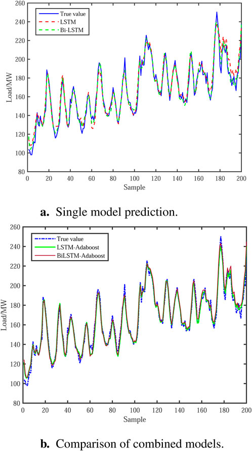
Figure 5 compares the viability of the hybrid forecasting method using a single and combined model. Figure 5A shows that in a single model, both the LSTM model and the Bi-LSTM model may fit loads. Bi-LSTM is more accurate than LSTM. When the load varies abruptly, resulting in a peak or peak valley, the single model cannot adequately anticipate; the inaccuracy is considerable, and there is some lag. Figure 5B shows that LSTM-Adaboost and Bi-LSTM-Adaboost models outperform other models in fitting load curves with peaks and valleys. At the same time, the combined model’s fitting curve is closer to the actual load at all times, demonstrating that the suggested method can better exploit the law and time aspects of load data. However, the effect of the two combined models is not significantly different, implying that the improved method’s optimization effect on LSTM and Bi-LSTM is comparable.

Figure 5

Figure 5. Comparison of models. (A) Single model prediction. (B) Comparison of combined models.

The models are assessed using MAE, MAPE, RMSE, and $R^2$. Table 5 summarizes the results. Table 5 shows that compared to LSTM and Bi-LSTM, MAE decreased by 2.0347 MW and 0.3658 MW, MAPE decreased by 1.207 $\%$ and 0.2211 $\%$, RMSE decreased by 2.7026 MW and 0.3699 MW, and $R^2$ increased by 0.03485 and 0.00376 respectively. Compared to the LSTM-Adaboost algorithm, MAE dropped by 0.2691 MW. MAPE reduced by 1.17 $\%$, RMSE decreased by 0.3626 MW, and $R^2$ increased by 0.00368, demonstrating the proposed method’s lower prediction error and improved accuracy.

Table 5

Table 5. Evaluation indexes of different models.

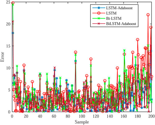
Figure 6 displays the relative absolute error distribution for each model. Figure 6 shows that this method has a lower relative absolute error and more steady load forecasting results than previous models. This is because the method presented in this paper employs VMD to decompose the sequence, remove the noise term, reduce the randomness of the sequence, and ensure that the sequence’s time characteristics are not discarded, allowing the Bi-LSTM model to be better used for error correction, resulting in a more detailed load forecasting process and improved load forecasting accuracy.

Figure 6

Figure 6. Four model prediction errors.

5.2 Ablation experiment

The ablation experiment of the method is equivalent to the control variable method. MIC, VMD, and Adaboost are used as the “variables” to be controlled, which are divided into the following three cases:

1. M1: MIC-Bi-LSTM-Adaboost was used and VMD was removed;

2. M2: VMD-Bi-LSTM-Aadboost was used and MIC was removed;

3. M3: MIC-VMD-Bi-LSTM was used and Adaboost was removed.

The results are shown in Table 6.

Table 6

Table 6. Ablation experiment results.

The table shows that all three techniques can enhance forecast accuracy. In comparison to M1, M2, and M3, Adaboost contributes the most to improving prediction accuracy. Compared to M1 and M2, selecting data meteorological elements can increase the prediction impact to some level, and removing factors with low correlation can minimize the number of principal components, simplify the method, and speed up prediction time. VMD primarily decomposes data and removes superfluous data, resulting in reduced algorithm complexity and improved prediction accuracy.

6 Conclusion

In this paper, a hybrid forecasting model according to MIC-VMD-Bi-LSTM-Adaboost is built by integrating the advantages of MIC, VMD, LSTM, Bi-LSTM and Adaboost. Firstly, the correlation analysis of meteorological factors influencing power load is ontained by using MIC, and the factors with higher correlation degree are extracted as input. Secondly, the input vector is decomposed by VMD to eliminate redundant data and extract features. Then, the Bi-LSTM-Adaboost fusion algorithm is applied to forecast the power load, calculate the error, and evaluate the model. Finally, the model is compared with two single algorithms of LSTM and Bi-LSTM and LSTM-Adaboost combination algorithm, so as to reflect the advantage of the algorithm in this paper. The following conclusions were reached:

1. MIC outperforms other correlation analysis functions in terms of computational complexity and robustness, providing significant advantages in correlation analysis. MIC chooses meteorological factors with high correlation as the input feature vector, which increases prediction accuracy in the subsequent combination process.

2. The Bi-LSTM network compensates for the LSTM network’s limitation of processing features in only one direction and outperforms it in terms of prediction effect.

3. Adaboost’s self-adaptability enhances the prediction accuracy of LSTM and Bi-LSTM, resulting in a more precise combined model than the individual models. The ablation experiment demonstrates that Adaboost contributes the most to the optimization algorithm in this research. The reason for this is that Adaboost may adaptively alter the anticipated error rate based on the weak classifier’s feedback, resulting in great execution efficiency.

4. The forecasting accuracy of the LSTM-Adaboost and Bi-LSTM-Adaboost algorithms is nearly same, showing that the Adaboost method has a similar influence on LSTM and Bi-LSTM optimization. Because of the lengthy prediction time of Bi-LSTM, LSTM can be combined directly in practical applications.

5. The combined approach suggested in this study outperforms the single algorithm in terms of accuracy, although there is still a significant inaccuracy at the start of the prediction. The evaluation coefficient is 0.97965, and there is still plenty of space for improvement. Future research will examine several aspects of the algorithm, including enhancing the attention mechanism, swapping out the GRU (Bi-GRU) algorithm, Transformer, and more.

Data availability statement

The datasets presented in this article are not readily available because the data set is urban power load, which is not disclosed in principle. Requests to access the datasets should be directed to ZY, MTkxMTI4NzQ4NTJAMTYzLmNvbQ==.

Author contributions

ZZ: Data curation, Formal Analysis, Writing–original draft, Writing–review and editing. CJ: Investigation, Methodology, Software, Writing–review and editing. YZ: Methodology, Supervision, Writing–review and editing. WW: Methodology, Supervision, Writing–review and editing. DH: Supervision, Validation, Writing–review and editing.

Funding

The author(s) declare that no financial support was received for the research, authorship, and/or publication of this article.

Acknowledgments

Authors sincerely acknowledge Measurement Center of Guangxi Power Grid Co., Ltd and NARI Group (State Grid Electric Power Research Institute) Co., Ltd.

Conflict of interest

Authors ZZ, CJ, and YZ were employed by Measurement Center of Guangxi Power Grid Co., Ltd. Authors WW and DH were employed by NARI Group (State Grid Electric Power Research Institute) Co., Ltd.

Publisher’s note

All claims expressed in this article are solely those of the authors and do not necessarily represent those of their affiliated organizations, or those of the publisher, the editors and the reviewers. Any product that may be evaluated in this article, or claim that may be made by its manufacturer, is not guaranteed or endorsed by the publisher.

References

Abumohsen, M., Owda, A. Y., and Owda, M. (2023). Electrical load forecasting using lstm, gru, and rnn algorithms. Energies 16, 2283. doi:10.3390/en16052283

CrossRef Full Text | Google Scholar

Aguilar Madrid, E., and Antonio, N. (2021). Short-term electricity load forecasting with machine learning. Information 12, 50. doi:10.3390/info12020050

CrossRef Full Text | Google Scholar

Álvarez, V., Mazuelas, S., and Lozano, J. A. (2021). Probabilistic load forecasting based on adaptive online learning. IEEE Trans. Power Syst. 36, 3668–3680. doi:10.1109/tpwrs.2021.3050837

CrossRef Full Text | Google Scholar

Bareth, R., Yadav, A., Gupta, S., and Pazoki, M. (2024). Daily average load demand forecasting using lstm model based on historical load trends. IET Generation, Transm. and Distribution 18, 952–962. doi:10.1049/gtd2.13132

CrossRef Full Text | Google Scholar

Chen, H., Wu, H., Kan, T., Zhang, J., and Li, H. (2023). Low-carbon economic dispatch of integrated energy system containing electric hydrogen production based on vmd-gru short-term wind power prediction. Int. J. Electr. Power and Energy Syst. 154, 109420. doi:10.1016/j.ijepes.2023.109420

CrossRef Full Text | Google Scholar

Cordeiro-Costas, M., Villanueva, D., Eguía-Oller, P., Martínez-Comesaña, M., and Ramos, S. (2023). Load forecasting with machine learning and deep learning methods. Appl. Sci. 13, 7933. doi:10.3390/app13137933

CrossRef Full Text | Google Scholar

Deng, S., Chen, F., Dong, X., Gao, G., and Wu, X. (2021). Short-term load forecasting by using improved gep and abnormal load recognition. ACM Trans. Internet Technol. (TOIT) 21, 1–28. doi:10.1145/3447513

CrossRef Full Text | Google Scholar

Deng, S., Chen, F., Wu, D., He, Y., Ge, H., and Ge, Y. (2022). Quantitative combination load forecasting model based on forecasting error optimization. Comput. Electr. Eng. 101, 108125. doi:10.1016/j.compeleceng.2022.108125

CrossRef Full Text | Google Scholar

Du, J., Cheng, Y., Zhou, Q., Zhang, J., Zhang, X., and Li, G. (2020). “Power load forecasting using bilstm-attention. IOP Conf. Ser. Earth Environ. Sci. 440, 032115. doi:10.1088/1755-1315/440/3/032115

CrossRef Full Text | Google Scholar

Ge, Q., Guo, C., Jiang, H., Lu, Z., Yao, G., Zhang, J., et al. (2020). Industrial power load forecasting method based on reinforcement learning and pso-lssvm. IEEE Trans. Cybern. 52, 1112–1124. doi:10.1109/tcyb.2020.2983871

CrossRef Full Text | Google Scholar

Geng, G., He, Y., Zhang, J., Qin, T., and Yang, B. (2023). Short-term power load forecasting based on pso-optimized vmd-tcn-attention mechanism. Energies 16, 4616. doi:10.3390/en16124616

CrossRef Full Text | Google Scholar

Guo, Y., Li, Y., Qiao, X., Zhang, Z., Zhou, W., Mei, Y., et al. (2022). Bilstm multitask learning-based combined load forecasting considering the loads coupling relationship for multienergy system. IEEE Trans. Smart Grid 13, 3481–3492. doi:10.1109/tsg.2022.3173964

CrossRef Full Text | Google Scholar

Habbak, H., Mahmoud, M., Metwally, K., Fouda, M. M., and Ibrahem, M. I. (2023). Load forecasting techniques and their applications in smart grids. Energies 16, 1480. doi:10.3390/en16031480

CrossRef Full Text | Google Scholar

Huang, X., Li, Z., Jin, Y., and Zhang, W. (2022). Fair-adaboost: extending adaboost method to achieve fair classification. Expert Syst. Appl. 202, 117240. doi:10.1016/j.eswa.2022.117240

CrossRef Full Text | Google Scholar

Jailani, N. L. M., Dhanasegaran, J. K., Alkawsi, G., Alkahtani, A. A., Phing, C. C., Baashar, Y., et al. (2023). Investigating the power of lstm-based models in solar energy forecasting. Processes 11, 1382. doi:10.3390/pr11051382

CrossRef Full Text | Google Scholar

Kumar, N. (2024). Ev charging adapter to operate with isolated pillar top solar panels in remote locations. IEEE Trans. Energy Convers. 39, 29–36. doi:10.1109/tec.2023.3298817

CrossRef Full Text | Google Scholar

Kumar, N., Mulo, T., and Verma, V. P. (2013). “Application of computer and modern automation system for protection and optimum use of high voltage power transformer,” in 2013 international conference on computer communication and informatics, 1–5.

CrossRef Full Text | Google Scholar

Kumar, N., Panigrahi, B. K., and Singh, B. (2016). A solution to the ramp rate and prohibited operating zone constrained unit commitment by ghs-jgt evolutionary algorithm. Int. J. Electr. Power and Energy Syst. 81, 193–203. doi:10.1016/j.ijepes.2016.02.024

CrossRef Full Text | Google Scholar

Kumar, N., Saxena, V., Singh, B., and Panigrahi, B. K. (2020). Intuitive control technique for grid connected partially shaded solar pv-based distributed generating system. IET Renew. Power Gener. 14, 600–607. doi:10.1049/iet-rpg.2018.6034

CrossRef Full Text | Google Scholar

Kumar, N., Saxena, V., Singh, B., and Panigrahi, B. K. (2023a). Power quality improved grid-interfaced pv assisted onboard ev charging infrastructure for smart households consumers. IEEE Trans. Consumer Electron. 69, 1091–1100. doi:10.1109/tce.2023.3296480

CrossRef Full Text | Google Scholar

Kumar, N., Singh, H. K., and Niwareeba, R. (2023b). Adaptive control technique for portable solar powered ev charging adapter to operate in remote location. IEEE Open J. Circuits Syst. 4, 115–125. doi:10.1109/ojcas.2023.3247573

CrossRef Full Text | Google Scholar

Lin, G., Lin, A., and Gu, D. (2022). Using support vector regression and k-nearest neighbors for short-term traffic flow prediction based on maximal information coefficient. Inf. Sci. 608, 517–531. doi:10.1016/j.ins.2022.06.090

CrossRef Full Text | Google Scholar

Madhukumar, M., Sebastian, A., Liang, X., Jamil, M., and Shabbir, M. N. S. K. (2022). Regression model-based short-term load forecasting for university campus load. IEEE Access 10, 8891–8905. doi:10.1109/access.2022.3144206

CrossRef Full Text | Google Scholar

Moreira-Júnior, J. R., Abreu, T., Minussi, C. R., and Lopes, M. L. (2022). Using aggregated electrical loads for the multinodal load forecasting. J. Control, Automation Electr. Syst. 33, 1592–1600. doi:10.1007/s40313-022-00906-1

CrossRef Full Text | Google Scholar

Nie, Y., Jiang, P., and Zhang, H. (2020). A novel hybrid model based on combined preprocessing method and advanced optimization algorithm for power load forecasting. Appl. Soft Comput. 97, 106809. doi:10.1016/j.asoc.2020.106809

CrossRef Full Text | Google Scholar

Park, K.-J., and Son, S.-Y. (2023). Residential load forecasting using modified federated learning algorithm. IEEE Access 11, 40675–40691. doi:10.1109/access.2023.3268530

CrossRef Full Text | Google Scholar

Rafi, S. H., Deeba, S. R., and Hossain, E. (2021). A short-term load forecasting method using integrated cnn and lstm network. IEEE access 9, 32436–32448. doi:10.1109/access.2021.3060654

CrossRef Full Text | Google Scholar

Satapathy, S. S., and Kumar, N. (2019). “Modulated perturb and observe maximum power point tracking algorithm for solar pv energy conversion system,” in 2019 3rd international conference on recent developments in control, automation and power engineering (RDCAPE) (IEEE), 345–350.

CrossRef Full Text | Google Scholar

Sukanya Satapathy, S., and Kumar, N. (2020). Framework of maximum power point tracking for solar pv panel using wsps technique. IET Renew. Power Gener. 14, 1668–1676. doi:10.1049/iet-rpg.2019.1132

CrossRef Full Text | Google Scholar

Surapunt, T., and Wang, S. (2024). Ensemble modeling with a bayesian maximal information coefficient-based model of bayesian predictions on uncertainty data. Information 15, 228. doi:10.3390/info15040228

CrossRef Full Text | Google Scholar

Tian, M.-W., Alattas, K., El-Sousy, F., Alanazi, A., Mohammadzadeh, A., Tavoosi, J., et al. (2022). A new short term electrical load forecasting by type-2 fuzzy neural networks. Energies 15, 3034. doi:10.3390/en15093034

CrossRef Full Text | Google Scholar

Wan, A., Chang, Q., Khalil, A.-B., and He, J. (2023). Short-term power load forecasting for combined heat and power using cnn-lstm enhanced by attention mechanism. Energy 282, 128274. doi:10.1016/j.energy.2023.128274

CrossRef Full Text | Google Scholar

Wang, Z., Wang, Q., and Wu, T. (2023). A novel hybrid model for water quality prediction based on vmd and igoa optimized for lstm. Front. Environ. Sci. and Eng. 17, 88. doi:10.1007/s11783-023-1688-y

CrossRef Full Text | Google Scholar

Wu, F., Cattani, C., Song, W., and Zio, E. (2020). Fractional arima with an improved cuckoo search optimization for the efficient short-term power load forecasting. Alexandria Eng. J. 59, 3111–3118. doi:10.1016/j.aej.2020.06.049

CrossRef Full Text | Google Scholar

Zhao, Z., Yun, S., Jia, L., Guo, J., Meng, Y., He, N., et al. (2023). Hybrid vmd-cnn-gru-based model for short-term forecasting of wind power considering spatio-temporal features. Eng. Appl. Artif. Intell. 121, 105982. doi:10.1016/j.engappai.2023.105982

CrossRef Full Text | Google Scholar