 Zhenxing Hu1
 Yizheng Zhao
 Liang Zhang
- 1China Electric Power Engineering Consulting Group Southwest Electric Power Design Institute Co., Ltd., Chengdu, China
- 2School of Electrical Engineering and Information, Southwest Petroleum University, Chengdu, China
The current carrying capacity of power cables is an important parameter for the operation and scheduling of power cables, which is limited by the maximum allowable operating temperature of the cables. Establishing a cable temperature field and current carrying capacity model considering the influence of airflow in complex environments is of great significance for studying cable current carrying capacity. Based on the coupling theory of electric field and heat flow field, a temperature field and current carrying capacity analysis model for high-voltage three core cross-linked polyethylene cable and its laying environment was established using finite element analysis technology. Studied the effects of external air velocity and temperature on the current carrying capacity of cables under two laying methods: direct burial and air laying. Research has shown that the allowable operating time of short-term emergency current carrying capacity of cables is positively correlated with their size, and inversely proportional to the initial temperature of the cable core. The steady-state and transient analysis results of this model provide important reference value for cable operation scheduling, and the correctness and effectiveness of the model have been further verified through experiments based on actual scenarios.
1 Introduction
Temperature and ampacity are two important dynamic operational parameters of power cables (Yongchun et al., 2012; Qin et al., 2022), which are related to the reliable and economical operation as well as the service life. At present, most power cables are crosslinked polyethylene (XLPE) cables, and their ampacity correspond to the operating current when the steady-state temperature of the cable core reaches 90°C (Zheng et al., 2010a). The calculation of the actual ampacity and the transient analysis of short-term emergency current are of great significance to optimize the construction cost and improve the utilization efficiency of cables (Wang, 2018).
The ampacity of the cable is closely related to the operating temperature, and the maximum operating temperature determines the ampacity of the cable (Ying and Cao, 2007; Zheng et al., 2010b). The analysis of temperature field and ampacity model of cable is a complicated electric-thermal-flow coupling problem. When current flowing through the cable, the temperature of the cable’s different structures increases due to conductor loss, insulation loss, metal sheath and armor loss. But the heat loss of cable is not only related with the parameters of the cable itself, but also related with the laying method and environmental parameters (Yongchun, 2016). In practice, there are two laying methods: burying and laying, and the effect of air current on the scouring and heat dissipation are different with different laying methods, which leads to differences on ampacity. Therefore, taking the influence of air current into consideration, when studying the temperature field and ampacity model is important to ensure the safe operation and improve the utilization efficiency of cables.
There are two main methods to analyze power cable temperature field and ampacity model: analytical calculation and numerical calculation (Callender et al., 2022; Che et al., 2022; Qin et al., 2022; Zhu et al., 2023; Zhu et al., 2024). The former is mainly based on the calculation of thermal resistance and related loss of each unit in IEC60287 standard. It also establishes the thermal circuit model of cables and combines the heat transfer formula to calculate the temperature field and ampacity of cables. However, the formulas in the IEC 60287 standard are so complicated, and they are not compatible to other laying methods and not available for the case of complicated laying environment. The numerical calculation method mainly includes finite element method (FEM), finite difference method (FDM), boundary element method (BEM) and so on. Compared with the other two methods, FEM is more suitable for dealing with complex boundary environment. It is convenient to analyze and calculate the temperature field and ampacity of cables with complex structures and laying environment, so that it has become a main method in this field in recent years. In reference (Qin et al., 2022), finite element simulation software was used to build an electromagnetic, thermal and current coupling model for 110 kV crosslinked polyethylene cable laid in the tunnel, and the temperature rise characteristics under different service years were analyzed. In reference (Che et al., 2022), using COMSOL multi physical field simulation software, the model of cable to calculate the current carrying capacity is established, and the relationship between cable capacity and temperature field is analyzed. On this basis, the influence of cable placement and convective thermal conductivity on temperature field distribution is further analyzed. In reference (Zhu et al., 2024), the finite element simulation software was used to analyze the variation of the operating characteristics of the electric field-temperature field-stress field of tunnel serpentine laying cables under different arc widths and pitches and their correlation with space occupancy. In reference (Zhu et al., 2023), The finite element simulation software is used to simulate the temperature field and stress field of parallel directly buried cables. cc.
In this paper, aiming at the high voltage three-core XLPE cable, according to the electrical-thermal-flow multi-field coupling theory, a temperature field and ampacity analysis model of cables considering laying environment is established based on finite element analysis. Ampacity differences caused by the two different laying methods at air current velocity of 0–2 m/s and air current temperature of 10–30°C are respectively studied. Taking the cable laying model as an example, the steady-state temperature of cables under different initial current is further analyzed, and the allowable time duration and variation of short-term emergency current of different magnitude are determined. The analysis and calculation of temperature field and ampacity in complex environment is helpful to improve the utilization efficiency of cables and provides important data support and reference values for dynamic capacity assessment and load dispatching.
2 Modeling electrical-thermal-flow multi-field coupling
The analysis of temperature field and ampacity model of cables in complex environment can be equivalent to the study of electrical-thermal-flow multi-field coupling between the cable itself and its laying environment. The following mathematical model is established to describe the process of heat generation in the conductor, heat conduction within the cable body, and convective heat transfer in flowing air current.
1) The model of electric field module can be formulated as:
In the formula: ∇ is the vector differential operator; J is the current density vector, A/m3;
2) The conductor, insulation, metal sheath and armor of cable produce loss and emit heat, and the heat is transmitted in the cable body. The mathematical model is as follows (Zhang et al., 2020):
In the formula: ρ is the density of the material, kg/m3; C is the specific heat capacity of the material at atmospheric pressure, J/(kg⋅m); T is the temperature of the material, K; λ is the thermal conductivity of the solid material, W/(m⋅K); Q is the heat source in the material, W/m3.
3) The heat is transferred from the cable body to the cable surface, and then the convective heat transfer with the air current occurs at the cable surface. Finally, the heat is transferred into the flowing air current. The model of air current heat transfer module can be formulated as (Yanbang et al., 2017):
In the formula: ρ1 is the density of the fluid material, kg/m3; C1 is the specific heat capacity of the fluid material at atmospheric pressure, J/(kg⋅m); T is the temperature of the material, K; v is the velocity vector, m/s; q is the conduction heat flux, W/m2; τ is the viscous stress tensor, Pa; S = 0.5 (∇v+(∇v)T) is the strain rate tensor, 1/s; p is the pressure, Pa; Q1 is the heat source in fluid materials (excluding viscous heating), W/m3.
3 Simulation model
3.1 Establishment of the finite element model
In this paper, the 35 kV three-core XLPE cable is taken as the main study object. Its actual structure is shown in Figure 1. The cable is mainly composed of the conductive wire core, optical fiber unit and outer material. From the inside to the outside, the conductive wire core is copper conductor, conductor shield, XLPE insulation layer, insulation shield, semi-conductive tape, alloy sheath and PE sheath. The outer materials from the inside to the outside are filling layer, cladding, PP inner cushion, armor, and PP outer coating.
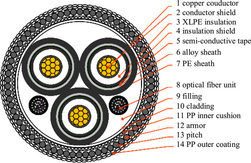
Figure 1. Schematic diagram of cable structure.
In order to reduce the computational burden of the finite element analysis and shorten the calculation time, the structural layers of cable with similar heat transfer coefficient and contact with each other are combined. The conductor shield, the XLPE insulation and the insulation shield are combined and collectively referred to as the insulation layer; the cladding and the PP inner cushion are combined and collectively referred to as the inner cushion layer. Figure 2 shows the geometric model of the merged cable, and Table 1 shows the structural performance parameters of the cable after combination.

Figure 2. Simplified model of cable.

Table 1. The performance parameters of each layer structure of cable.
In the simulation analysis of the temperature field and the current carrying capacity of the cable, the finite element model with certain laying methods should be established, including the burying and laying of the cable. The cable laying environment is equivalent to two different layers of material, the upper layer is “air current,” including one inlet and one outlet, and the lower layer is “soil area.” When the burying method is adopted, the burying depth is more than 0.5 m; when the laying method is adopted, the cable is laid flat on the soil, while considering the gravity the cable will slightly sink in the soil. Previous studies have shown that areas more than 2 m away from the cable are not affected by cable heating (Xu, 2013). The cable analysis models of two different laying methods are shown in Figure 3.
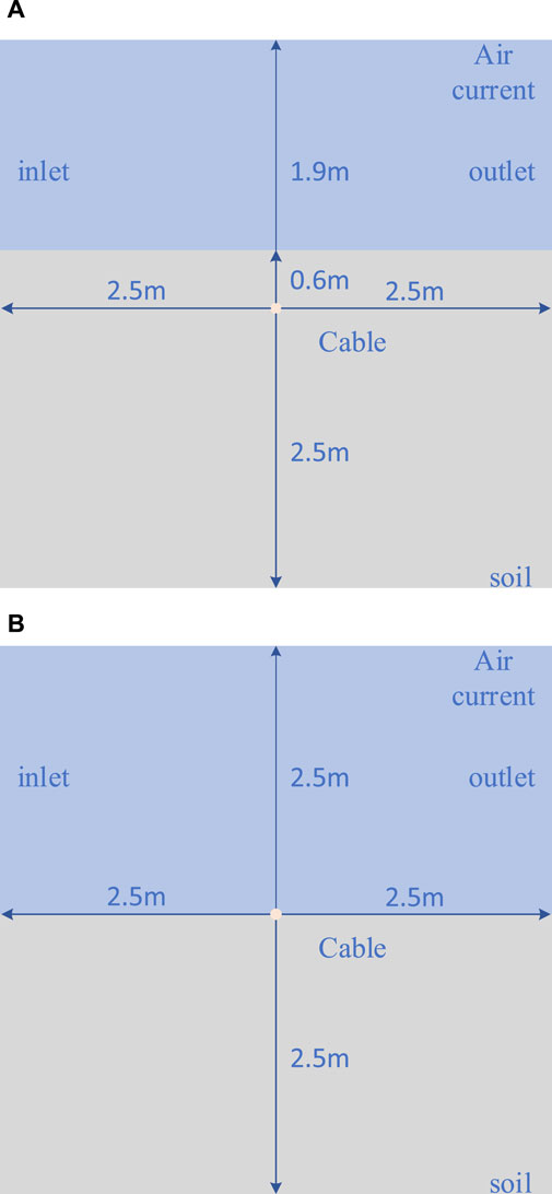
Figure 3. Cable analysis model under different laying methods. (A) The model of buried cable. (B) The model of cable during laying.
3.2 Meshing and boundary condition setting
The calculation of the finite element analysis is carried out in the grid element, and the higher the density of the grid, the higher the accuracy, while the computational burden and time will correspondingly increase. In this paper, a higher density gird is applied in analyzing the cable itself and important parts surrounding it, and a relatively low density grid is applied on the distant air current and soil areas, which ensures the accuracy of the temperature field and ampacity calculation of the cable, while reducing the computational burden and time. The schematic diagram of the grid density is shown in Figure 4.
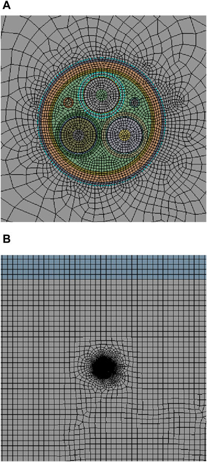
Figure 4. Schematic diagram of grid division. (A) Local grid density map of the cable. (B) Global grid density map.
The finite element analysis model of temperature field and ampacity includes the following three modules, and the specific boundary conditions are set as follows.
(1) Electrical field module: voltage level of 35 kV is applied to the conductor of the cable to inject current in the form of normal current density.
(2) Flow module: Let the air current flows in from the left interface of the air current region and flows out from the right interface; there is no air current flowing in or out from other interfaces.
(3) Heat transfer module. The boundary under the overall model of submarine cables and their laying environment is a constant temperature of 15°C, which is the first type of thermal boundary condition. The horizontal temperature gradient at the left and right boundaries of the overall model is 0, which is the second type of thermal boundary condition. In the model, the upper boundary of the soil directly convective heat transfer with the air, with a heat transfer coefficient of 5 W/(m2•K), is the third type of thermal boundary condition.
4 Experimental verifications
4.1 Example analysis
Taking Qinhuangdao as an example, the annual average temperature (Ta) is 22°C; air velocity (v0) is 0.8 m/s; and bottom temperature (Tb) is 20°C. Based on the above settings, the ampacity (Is) under two different laying environments can be calculated. Figure 5 shows the local temperature cloud map of the ampacity under two different laying environments based on finite element analysis model, corresponding to 604.89A and 935.65A.
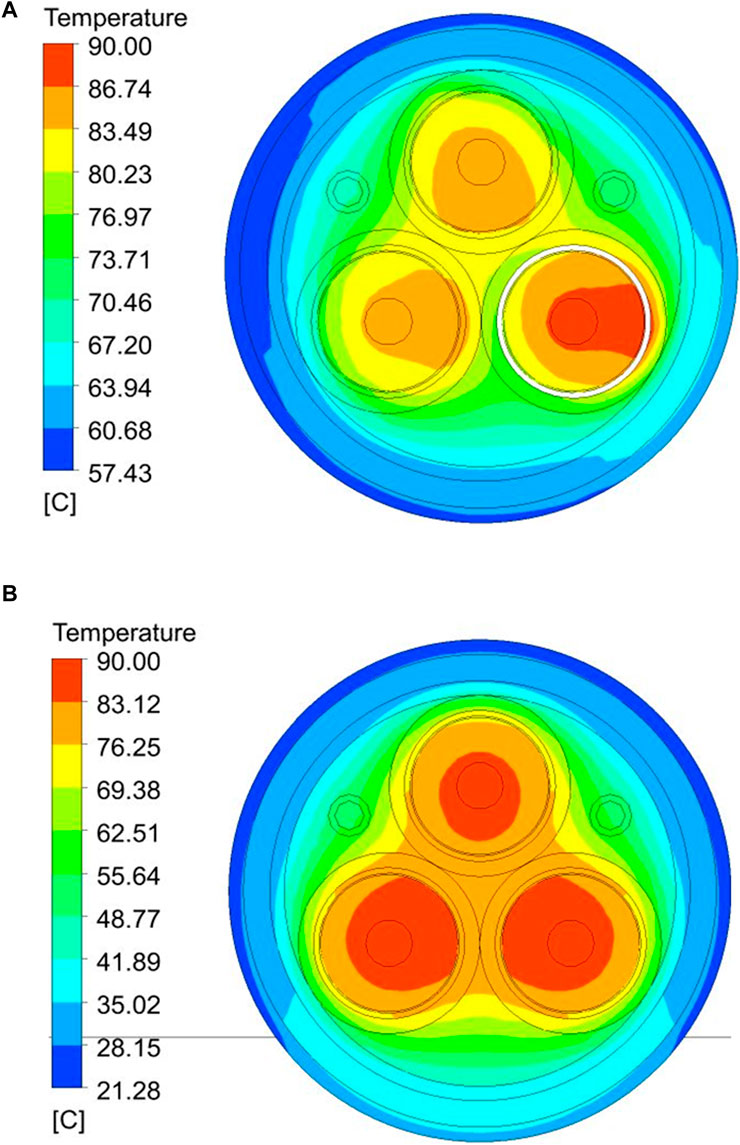
Figure 5. Local temperature cloud map of cable under ampacity. (A) Local temperature distribution of buried cable. (B) Local temperature distribution of cable during laying.
As shown in Figure 5, due to the low thermal conductivity and high specific heat capacity of the soil in the buried state, the heat generated by the cable is difficult to transfer, resulting in a high surface temperature of about 57.43°C; Under the laying method, the steady-state temperature field is more distributed, and the surface temperature is about 21.28°C, which is almost the same as the air temperature.
The formula of the analytical method for the ampacity calculation of AC cables in IEC60287 standard is shown as (6). Its calculation results and relative errors are shown in Table 2.
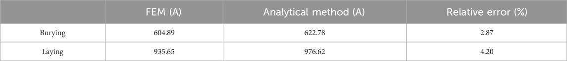
Table 2. Comparison of the calculation results of ampacity.
In the formula,
It can be seen from Table2, the calculation results of the FEM, and the analytical method are close and their relative errors are all within the range of engineering requirements (5%).
4.2 Steady-state analysis of ampacity in complex environment
In the case of laying method, the main environmental factors that affect the temperature field distribution and ampacity of the cable are air current velocity and temperature.
4.2.1 Analysis of the influence of air current velocity
In order to quantitatively analyze the effect of air flow velocity on cable current carrying capacity, we set Tb = 20°C and control the inlet flow velocity v0 in the air area to be between 0 and 2 m/s. We determined the steady-state current carrying capacity of cable burial and air under different flow velocities, and the results are shown in Figure 6.
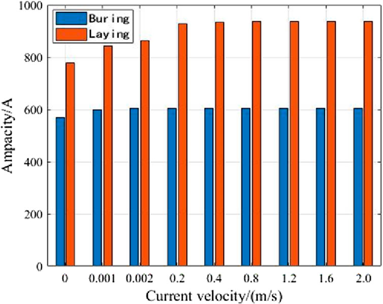
Figure 6. Ampacity of cable at different current velocity.
Under the condition of v0 = 0 m/s,
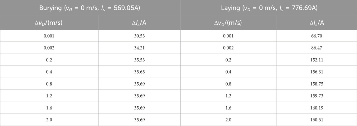
Table 3. The relationship between ampacity of cable and air velocity.
It can be seen from Table 3 that no matter when the cable is buried or laid, a slight change in air current velocity will lead to a significant increase in Is of the cable compared with v0 = 0 m/s. Moreover, the air current velocity is different and the degree of rise is different. The influence of the air current velocity is much greater in the low velocity range than in the high velocity range, but it will soon reach the bottleneck, that is, when the air current flow rate is greater than 0.2 m/s, the steady-state capacity changes tend to be stable.
Under different laying methods, the ampacity of cables could increase with different degrees with the change of air current velocity. The reason is that under the burying method, the heat generated by the ampacity of cable is transmitted into the soil, having only a small share transferred to the surface of the soil, which is carried away by air flow. However, under the laying method, the heat is directly carried away by the air flow, which explains the higher ampacity than the burying method. In addition, under the same air current velocity change, the ampacity increase is more significant as well.
4.2.2 Analysis of the influence of air current temperature
Air current temperature is another important factor in the analysis of temperature field and ampacity model. We set v0 as 0.8 m/s and increase air current temperature from 10°C to 30°C with a step of 1°C to study the change of ampacity under different air current temperatures.
Figure 7 shows the variation of ampacity of buried and laid cables at different air current temperatures. It can be seen from the figure that: 1) Is decreases slightly when buried; 2) under the same air temperature,
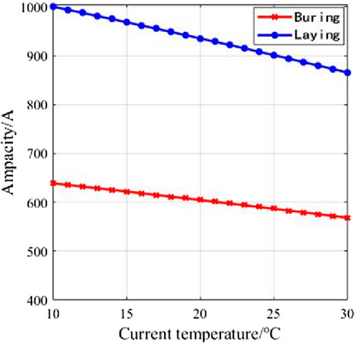
Figure 7. Ampacity of cable under different air temperature.
It is clear from the formula that the first term coefficient between Is and the air current temperature is −3.519 while the cable buried, and it is −6.733 while the cable laid.
4.3 Transient analysis of short-term emergency current
During normal operation of the cable, the temperature of the cable is lower than the maximum allowable temperature because it is usually not the maximum current carrying capacity. The maximum current carrying capacity can be exceeded for a short time if economical permits, although this will lead to increased heating of the cable, but the accumulation in a short time will not cause the cable to be heated above the allowable temperature.
In order to analyze the transient process of core temperature under different initial currents and determine the allowable operating time of short-term emergency currents of different sizes, this paper takes the cable analysis model under laying methods as an example. We set v0=0.8 m/s and respectively set air current temperature and deep soil temperature as 20°C and 15°C. The overall initial temperature of the cable is set as 16.67°C. The steady-state core temperature is determined when the initial current is 80%, 85%, 90%, and 95% of Is. The results are shown in Table 4.

Table 4. Steady-state cable core temperature under different initial current.
It can be seen from the results that the steady-state cable core temperature increases uniformly with the increase of initial carrying capacity. On the basis of this steady state, the emergency carrying capacity of 1.05Is, 1.10Is, 1.15Is, and 1.20Is is applied respectively in this specific environment to keep the cable core temperature constant after reaching 90°C, and the temperature rise process of the cable core is shown in Figure 8.
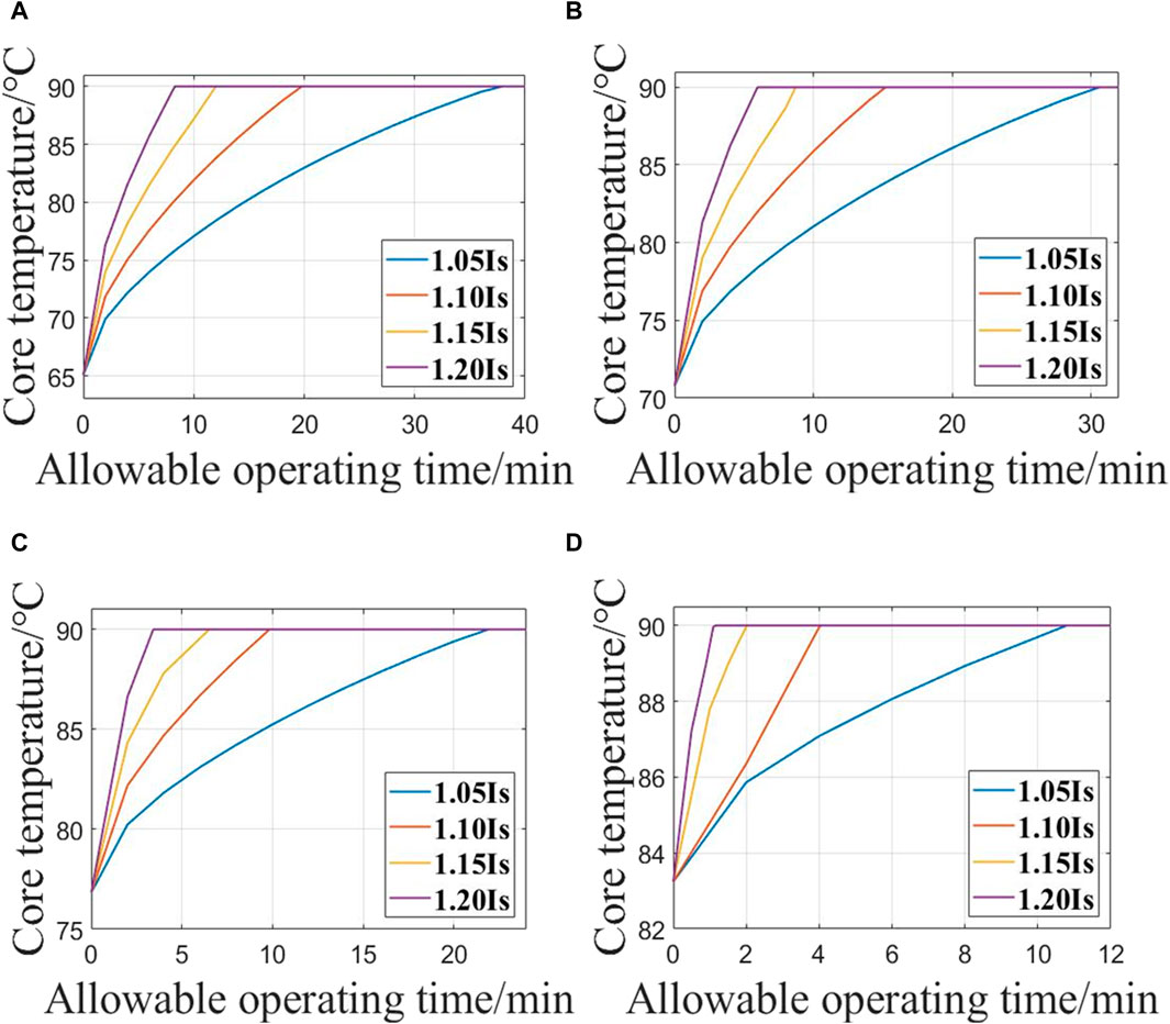
Figure 8. The rising process of cable core temperature under different current. (A) Initial current = 80%Is. (B) Initial current = 85%Is. (C) Initial current = 90%Is. (D) Initial current = 95%Is.
It can be seen from Figure 8 that with the same initial ampacity, the greater the emergency current, the shorter the time taken by the cable core to reach the upper temperature limit of 90°C. The allowable operation time of the emergency ampacity is impacted by the initial ampacity Figure 9 shows the allowable operating time of emergency current under different conditions.
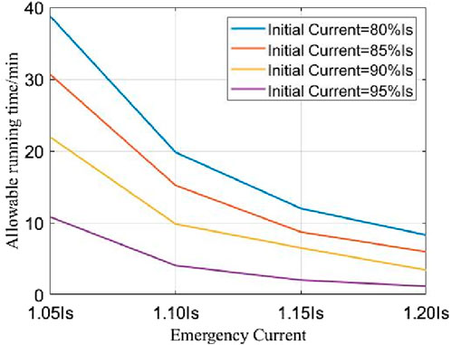
Figure 9. Allowable operating time of emergency current under different conditions.
It can be seen from the results that the allowable running time of the same emergency carrying capacity gradually decreases with the increase of the initial carrying capacity. When the emergency load capacity Is 1.05Is, when the initial load capacity is increased by 5%Is, the allowable running time is reduced by 8.73 min on average. With the increase of emergency load capacity, the allowable running time decreases greatly. When the emergency load capacity Is 1.20Is, the allowable running time is less than 10min. Especially when the initial load capacity is 95% Is, the allowable running time is only 1.18 min.
5 Conclusion
In this paper, aiming at the 35 kV three-core XLPE cable, the temperature field and ampacity analysis model of cable and its laying environment are established based on finite element analysis technology. The proposed model can not only analyze and calculate the temperature field and the steady-state and transient results of the ampacity under different laying methods, but also the calculation is fast and efficient. The study is helpful to the reasonable scheduling planning of cable real-time operation, and the following conclusions are drawn.
1) Under the same environmental parameters, the steady-state carrying capacity of the cable in the air is 200–330A higher than that when the cable is buried.
2) Considering the temperature range of air current at the actual laying depth of cable, there is an almost linear relationship between the ampacity and the temperature of air current, that is the ampacity decreases linearly as the temperature of air current increases.
3) The allowable operating time for short-term emergency current of different magnitude of cable is inversely proportional to its magnitude and the initial core temperature. The allowable operating time of the emergency current of the same magnitude decreases uniformly with the increase of the initial current, and the larger the emergency current, the shorter the allowable operating time.
Data availability statement
The original contributions presented in the study are included in the article/Supplementary Material, further inquiries can be directed to the corresponding author.
Author contributions
ZH: Writing–review and editing. XY: Writing–review and editing. QL: Writing–original draft. XL: Writing–review and editing. YZ: Writing–original draft. HZ: Writing–review and editing. LZ: Writing–review and editing.
Funding
The author(s) declare that no financial support was received for the research, authorship, and/or publication of this article.
Acknowledgments
This research thanks for the comments from reviewers. The authors would like to take this opportunity to thank the data collection assistants and the anonymous respondents who responded to the questionnaire.
Conflict of interest
Authors ZH, XY, XL, and HZ were employed by the China Electric Power Engineering Consulting Group Southwest Electric Power Design Institute Co., Ltd.
The remaining authors declare that the research was conducted in the absence of any commercial or financial relationships that could be construed as a potential conflict of interest.
Publisher’s note
All claims expressed in this article are solely those of the authors and do not necessarily represent those of their affiliated organizations, or those of the publisher, the editors and the reviewers. Any product that may be evaluated in this article, or claim that may be made by its manufacturer, is not guaranteed or endorsed by the publisher.
References
Callender, G., Goddard, K. F., Dix, J. K., and Lewin, P. L. (2022). A flexible model to calculate buried cable ampacity in complex environments. IEEE Trans. Power Deliv. 37 (3), 2007–2015. doi:10.1109/tpwrd.2021.3102414
Che, C., Yan, B., Fu, C., Li, G., Qin, C., and Liu, L. (2022). Improvement of cable current carrying capacity using COMSOL software. Energy Rep. 8 (15), 931–942. doi:10.1016/j.egyr.2022.10.095
Qin, S., Xu, Q., Wang, Q., Zhang, J., Ju, Z., Hou, Z., et al. (2022). Study on temperature rise characteristics of 110 kV XLPE cable under different service years considering dielectric loss. Energy Rep. 8 (8), 493–501. doi:10.1016/j.egyr.2022.09.153
Wang, Q. (2018). Analysis and research on dynamic ampacity of cable. Shenyang University of Technology.
Xu, ZHANG (2013). Research on fault simulation of photoelectric composite submarine cable[D]. North China Electric Power University.
Yanbang, H. A. O., Chen, Y., Yang, L., Qiu, W., Fu, M., and Hou, S. (2017). Coupled simulation on electro-thermal-fluid multiple physical fields of HVDC submarine cable. High. Volt. Eng. 43 (11), 3534–3542. doi:10.13336/j.1003-6520.hve.20171031007
Ying, L., and Cao, X. (2007). Research and application of online temperature and load monitoring for power cables. Power Syst. Clean Energy 23 (4), 11–14.
Yongchun, L. (2016). Technological development in evaluating the temperature and ampacity of power cables. High. Volt. Eng. 42 (4), 1142–1150. doi:10.13336/j.1003-6520.hve.20160405014
Yongchun, L., Zhao, J., and Caihong, Y. (2012). Numerical calculation of temperature field and ampacity of power cables in channel. High. Volt. Eng. 38 (11), 3048–3053. doi:10.3969/j.issn.1003-6520.2012.11.037
Zhang, L., He, Y., Liu, Y., Yang, F., He, T., Liu, L., et al. (2020). Temperature analysis based on multi-coupling field and ampacity optimization calculation of shore power cable considering tide effect. IEEE Access 8, 119785–119794. doi:10.1109/access.2020.3005305
Zheng, Y., Ning, W., Hongjie, L., and Zhang, G. (2010a). Study and progress of the ampacity computation of power cables. Electr. wire cable (2), 4–9. doi:10.16105/j.cnki.dxdl.2010.02.008
Zheng, Y., Wang, N., Hongjie, L., and Zhang, G. (2010b). Methods and progress of the ampacity computation of power cables. Electrotech. Appl. 29 (3), 26–31.
Zhu, H., Han, Z., Yang, J., Zhang, R., Liu, C., Chen, W., et al. (2023). Multi-factor simulation analysis of operation characteristics of side-by-side directly buried cables. Electr. Power Syst. Res. 218, 109143. doi:10.1016/j.epsr.2023.109143
Keywords: power cable, temperature field, electro-thermal-flow coupling, finite element analysis, steady-state ampacity, short-term emergency current
Citation: Hu Z, Ye X, Li Q, Luo X, Zhao Y, Zhang H and Zhang L (2024) Analysis on three-core power cable temperature field and ampacity model under typical laying environment. Front. Energy Res. 12:1430501. doi: 10.3389/fenrg.2024.1430501
Received: 10 May 2024; Accepted: 30 May 2024;
Published: 11 July 2024.
Edited by:
Wei Qiu, Hunan University, ChinaReviewed by:
Baohong Li, Sichuan University, ChinaJianfeng Liang, Xi’an University of Technology, China
Copyright © 2024 Hu, Ye, Li, Luo, Zhao, Zhang and Zhang. This is an open-access article distributed under the terms of the Creative Commons Attribution License (CC BY). The use, distribution or reproduction in other forums is permitted, provided the original author(s) and the copyright owner(s) are credited and that the original publication in this journal is cited, in accordance with accepted academic practice. No use, distribution or reproduction is permitted which does not comply with these terms.
*Correspondence: Qian Li, c3dwdWxpcWlhbkAxNjMuY29t