 Yafangzi Zhou1
 Zhiyin Su
94% of researchers rate our articles as excellent or good
Learn more about the work of our research integrity team to safeguard the quality of each article we publish.
Find out more
ORIGINAL RESEARCH article
Front. Energy Res. , 17 June 2024
Sec. Smart Grids
Volume 12 - 2024 | https://doi.org/10.3389/fenrg.2024.1423692
This article is part of the Research Topic Advances in Renewable Energy System Monitoring, Situational Awareness, and Control View all 21 articles
Short-term power load forecasting is the basis for ensuring the safe and stable operation of the power system. However, because power load forecasting is affected by weather, economy, geography, and other factors, it has strong instability and nonlinearity, making it difficult to improve the accuracy of short-term power load forecasting. To solve the above problems, a load forecasting method combining empirical modal decomposition (EMD) and long short-term memory neural network (LSTM) has been proposed. The original signal is first decomposed into a series of eigenmode functions and a residual quantity using the EMD algorithm. Subsequently, all the components are fed into the LSTM network. To further improve the load prediction accuracy, a self-attention mechanism is introduced for large component signals to further explore the internal correlation of the data, and the Sparrow Optimisation Algorithm (SSA) is used to optimize the LSTM hyperparameters. Combining EMD, LSTM, self-attention mechanism (SAM), and SSA, the EMD-SSA- SAM -LSTM method for short-term power load forecasting is further proposed. The results show that the coefficient of determination (R2) of the method is 0.98, the mean absolute error (MAE) is 0.013, the root mean square error (RMSE) is 0.018, and the mean absolute percentage error (MAPE) is 2.57%, which verifies that the proposed model can improve the accuracy of load forecasting, and has a certain application prospect.
Accurate short-term power load forecasting is crucial to the economical, safe, and stable operation of the power system. In recent years, with the continuous development of clean energy, distributed energy in the power grid is increasing, resulting in new energy consumption in the power grid, transformer heavy overload and main transformer reverse power delivery and other problems are becoming more serious. To solve the above problems, the relevant departments of the State Grid should formulate an orderly power consumption plan, and reasonably arrange the power generation, transmission, and power supply, and these plans are highly dependent on the accurate power load forecast. Therefore, it is important to improve the accuracy of power load forecasting.
Since short-term power loads are commonly used in daily or weekly scheduling plans, which have a guiding effect on the grid scheduling department, most domestic and international researchers are committed to improving the accuracy of short-term power load forecasting. Traditional load forecasting methods include exponential smoothing, autoregressive integral sliding average model, multiple linear regression, and Weighted Moving Average (Chapagain and Kittipiyakul, 2018; Lee et al., 2018; Rosnalini et al., 2019; Nuo et al., 2023). Although these methods have good interpretability and fast computational speed, these methods are less robust and perform poorly in predicting large amounts of data and sudden power loads (Nuo et al., 2023). With the development of deep learning and the improvement of computer arithmetic power, deep learning has become a mainstream load forecasting method. Deep learning-based time series prediction methods include Convolutional Neural Networks (CNN), Recurrent Neural Networks (RNN) (Kang et al., 2020), Long Short-Term Memory (LSTM) (Gan et al., 2017; Kong et al., 2018), and Transformer, among others. The above methods are either capable of extracting features of time series or enabling memory of time series through gating units, all of which make them sensitive to time series data. Moreover, LSTM is the most commonly used load forecasting algorithm because it can solve the gradient explosion and gradient vanishing phenomena in RNN by extracting the time series features through input gates, memory gates, and output gates (Torres et al., 2021). For example, Xu Wu et al. added the Global Context Transformer module to LSTM for short-term wind power prediction while cleaning the data, and improved the prediction error in 12h and 24 h prediction, respectively (Wu et al., 2023). Wang Ye et al. used a multilayer inflated LSTM network combined with an attention mechanism for short-term power load forecasting and finally verified the effectiveness of the proposed method (Ye et al., 2023).
Due to the poor generalisation ability of individual LSTM models and the numerous hyperparameters of LSTM that are difficult to tune, some researchers have worked on combining LSTM with other methods. One common practice is to combine LSTM with other neural networks for time series prediction. For example, Ding Guili et al., 2023 combined a convolutional neural network with the pooling of multilayer spatial pyramids and LSTM with the allocation of attention mechanism for short-term power prediction of wind farm clusters and finally proved experimentally that the method can effectively improve the prediction accuracy of wind farm clusters under excessive weather. Zhong Bin proposed combining an artificial neural network, LSTM, and Transformer for power load prediction and finally verified the effectiveness of the method through multiple datasets (Bin, 2023). Jun Tang et al., 2024 combined the local attention mechanism with LSTM for short-term load prediction of total electron content in the ionosphere, and the time series prediction method was able to have good prediction stability under different geomagnetic conditions and different months. Another approach is to combine LSTM with signal decomposition methods. For example, Cheng Nuo et al. proposed the combination of variational modal decomposition, Prophet, and LSTM for electric vehicle load forecasting, which can effectively improve load forecasting accuracy compared with traditional methods (Nuo et al., 2023). Zhiyi Zhou et al. combined empirical modal decomposition (EMD) and LSTM for short-term wind power prediction, which can effectively improve the accuracy of wind power prediction (Zhou et al., 2023).
To improve the load prediction accuracy in one step, some approaches combine optimization algorithms with LSTM to optimize the hyperparameters of LSTM. For example, Zhang Daohua et al. Use Bayesian optimization of hyperparameters of CNN-BiLSTM for smart grid load forecasting (Xiao et al., 2024a). Yong Mao Zhu et al. used a particle swarm optimization algorithm to optimize the hyperparameters of LSTM for power load forecasting and demonstrated that the method can improve load forecasting accuracy (Xiao et al., 2024b). Based on the above studies, considering the inherent nonlinearity of power loads themselves and the fact that EMD can decompose non-smooth signals into a series of intrinsic modal functions (Zhou et al., 2023), the article combines EMD with LSTM for load forecasting to reduce the nonlinearity of loads. In addition, for large component signals article also introduces Self-Attention Mechanism (SAM) and Sparrow Search Algorithm (SSA), which are used to further explore the relationship between different batches of data and to enhance the generalisation ability of the model, respectively, and finally form the EMD-SSA-SAM-LSTM method for load prediction. The contributions of this paper are as follows:
1) Combining EMD with deep learning algorithms reduces the bilinearity and instability of raw load data.
2) Introducing SSA to optimise hyperparameters of deep learning algorithms to improve generalisation of load forecasting models.
3) Combine SAM with LSTM to further mine the correlation between different batches of samples.
The remaining parts of this paper are arranged as follows: the second part mainly introduces the theoretical background of the load forecasting method in this paper, the third part introduces the overall framework of the load forecasting method in this paper, the fourth part is the experiments and analyses of the EMD-SSA-SAM-LSTM forecasting model, and the fifth part asks for a summary of the paper.
In this section, the principle of EMD and SSA, the model architecture of Attention and LSTM are introduced.
The raw load data is firstly input into EMD and decomposed into several smoothed signals. Where EMD is mainly used to analyze non-stationary and non-linear signals (Zhou et al., 2023). The raw signal is decomposed into a series of eigenmode functions and a residual term. The computational equation is given below
where A is the original signal, IMFm is the mth eigenmode function, and Residual is the residual term.
The schematic diagram of the first eigenmode function obtained by EMD decomposition is shown in Figure 1, where the black curve is the real curve of the load noted as S1, the red curve is the curve of the extreme value and the curve of the very small value of the real value of the load noted as S2 and S3, respectively, and the blue curve is the average of the curves of the very large value and the very small value of the curve noted as S4. The specific decomposition steps are as follows:
1) For a given original signal, find the maximum and minimum value points, and form the maximum and minimum value envelopes to obtain S2 and S3;
2) Average the maximum and minimum envelopes to obtain S4;
3) Subtract S4 from the original signal to obtain a new signal called S5, if S5 meets the requirements of the eigenmode function, the decomposition is completed, and S5 is used as the first eigenmode function. Otherwise, continue the above steps with S5 until the first eigenmode function is obtained;
4) Subtract the first eigenmode function from the original signal to form a new signal, and use the new signal as the original signal in the above operation. Finally, a series of eigenmode functions and a residual term are obtained, i.e., several signals that are smoother than the original signal.
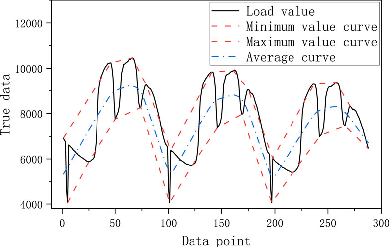
Figure 1. EMD decomposition principle.
The decomposed signal is divided into a large component signal and a small component signal, where the large component signal and the small component signal differ by one order of magnitude, and the large component signal is input to the SAM and the small component signal is input to the LSTM. Among them is the Attention Mechanism, which is an approach to mimic human attentional behavior and is used in deep learning to process sequential and other structured data (Vaswani et al., 2017). For time series data, the core idea of the attention mechanism is to extract the data that is relevant to the current data, while giving smaller weights to irrelevant data to determine the query, keyword, and answer matrices through training.
The schematic diagram of the multiple heads attention mechanism is shown in Figure 2, where Q, K, and V denote Query, Key, and Value respectively. Denotes query, keyword, and answer respectively. Multiple heads denote the number of multiple heads of the self-attention mechanism. The expression formula is as follows.
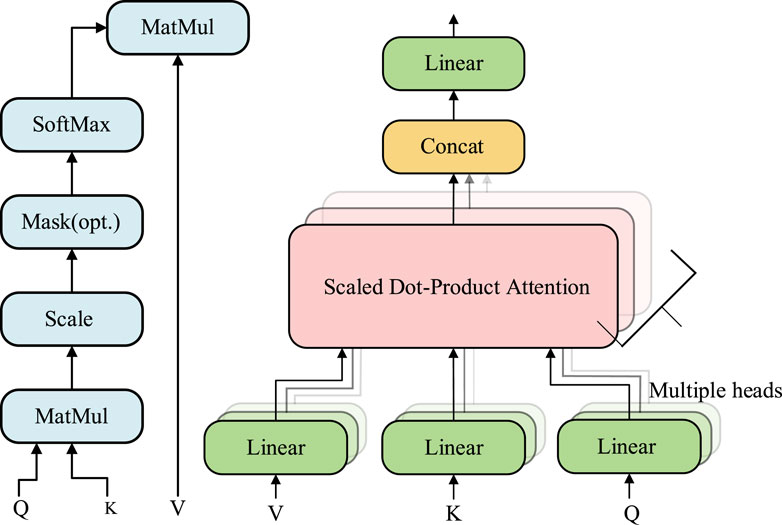
Figure 2. Self-attention mechanism principle flowchart.
Where X denotes the input vector and WQ, WK, and WV denote the initialized weight matrices of Q, K, and V.
Finally, the result of the dot product attention mechanism can be calculated based on the Q, K, and V vector values as shown in the following equation.
where dk denotes the word vector dimension of Q and K.
Secondly, the computational procedure for the multiple attention mechanism is as follows.
where headn denotes the nth level of multi-head operation. After the self-attention mechanism for joining the LSTM layer after the self-attention mechanism layer a fully connected layer is added.
The EMD-decomposed small signals and the SAM-composed large-component signals are input into different LSTM models for prediction, respectively. Among them, the LSTM model is developed from RNN, which avoids the problems of gradient vanishing and gradient explosion in RNN backpropagation to a certain extent (Torres et al., 2021).
The LSTM minimal cell is shown in Figure 3, where σ is a sigmoid function, Ct is the memory information output by this cell, ht is the output of this cell, Ct-1 is the memory information output by the previous cell, ht-1 is the output of the previous cell, mt denotes the input data of this cell, and tanh is an activation function.
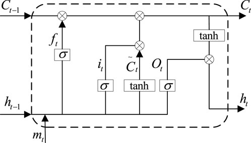
Figure 3. LSTM minimal cell.
Where the sigmoid function and the tanh function as
The input information of this cell and the output information of the previous cell are superimposed and the useless information is filtered out by the sigmoid function as
where Wf and bf are the weight matrix and bias matrix, respectively.
The input gate determines the extent to which the current input data enters the cell state, and the data updates the cell state through the input gate which is.
The memory information of this cell is updated through the superposition of the forgetting gate and the input gate, as follows.
The output of the LSTM unit is integrated by a stack of updated memory information and input information, which can be expressed as.
The output of each LSTM unit is linked to the next layer of a neural network to finally get the output of the model.
SSA is a population intelligence optimization algorithm that mimics sparrow foraging. In this paper, the sparrow search algorithm is used to optimize the hyperparameters of LSTM. The specific principles of sparrow search will be described below.
As shown in Eq. 16, using the matrix X to represent the sparrow population.
Where n denotes the number of sparrow populations, d denotes the number of LSTM hyperparameters to be optimized, and x denotes each sparrow in the sparrow population.
Based on the hyperparameters of each set of LSTMs, n fitness function values can be obtained, which can be expressed as.
Within this set of fitness functions, there is a best fitness function, that is, a set of hyperparameters of the LSTM for which the fitness function takes the smallest value, which can be described as
After that, the sparrow population will be divided into two kinds, the sparrows that are closer to the best fitness function are called discoverers, and the sparrows that are farther away from the best fitness function are called followers. After obtaining the best fitness function, the position of the discoverer and the follower will be changed, where the position of the discoverer is updated as follows
Where itermax denotes the set maximum number of iterations set in the sparrow search algorithm, α denotes a uniform random number of [0,1], Q denotes a standard normal random number, R2 denotes that a predator is a random number of [0,1], ST denotes the value of the warning that the finder has found the predator, xi, jt+1 denotes the position after the update, and xi, jt denotes the position before the update.
The follower positions have been updated as follows
Where xtworst denotes the sparrow that represents the least adapted sparrow in the current population and xtbest denotes the best adapted sparrow in the current population.
Eventually, a set of LSTM parameters for optimal fitness is found through continuous iterative updating.
The specific process is shown in Figure 4 as a flow chart of the procedure, where a is the current iteration number of SSA, which can be divided into four steps:
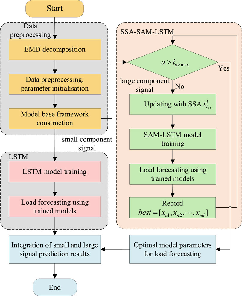
Figure 4. Program flow chart.
Step 1: First, the raw load data is decomposed into several small component signals and one large component signal using EMD; Each component is spliced with the feature data and subjected to data deletion, addition and normalisation, where the normalisation process uses the maximum-minimum-value normalisation method to normalise the data to [0,1]; And the initial LSTM load prediction model framework is constructed.
Step 2: Secondly, the decomposed signals are divided into large-component signals and small-component signals, and the small-component signals are predicted using the traditional LSTM model; The dataset is divided into a training set and a validation set, and the data from the training set is used to train the LSTM model by the Adam’s Gradient Descent Algorithm; then the loads are predicted on the small-component signals using the trained model. It is worth mentioning that Adam is one of the most popular and commonly used optimisers for neural network training, which adjusts the learning rate based on historical gradient information and combines the advantages of AdaGrad and RMSProp to improve the efficiency of model training. And the dropout layer is introduced in the model training process to prevent the normalisation phenomenon.
Step 3: Again, the SSA-SAM-LSTM model is used for prediction for large component signals; first determine whether SSA reaches the maximum number of iterations, and if it fails to do so, update the parameters of the LSTM model to be optimized through SSA, use the SAM-LSTM model for load prediction, and record the optimal fitness value and corresponding model parameters in the current sparrow population; if the maximum number of iterations has been reached, then use the LSTM model parameters under the optimal fitness value for load prediction to obtain the load prediction results under large component. Number of iterations, then use the LSTM model parameters under the best fitness value for load prediction and obtain the load prediction results under a large fraction.
Step 4: Finally, the load forecast results of the small component are combined with the load forecast results of the large component to obtain the final load forecast results.
The shape of the input data for the model is shown in Figure 5, where the horizontal axis is the number of features F, the vertical axis is the time step T, and the vertical axis is the length of the input data S.
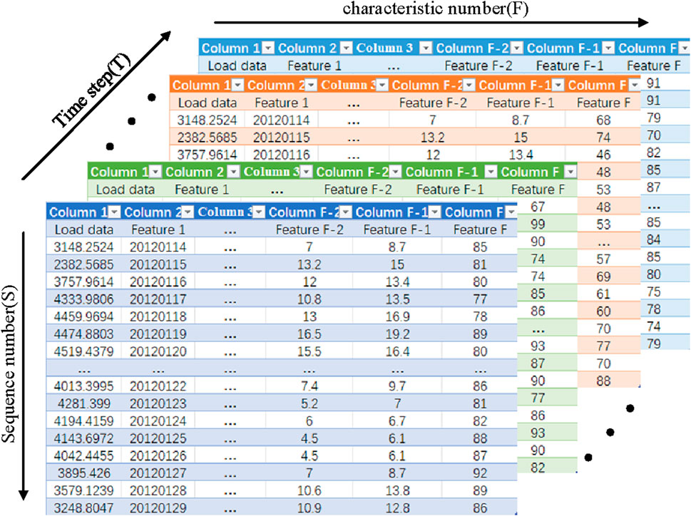
Figure 5. Model input data shape.
If time is considered as a dimension, the input to the model is three-dimensional data, while the input to the model at a given point in time is two-dimensional data, and one of the dimensions of that two-dimensional data is the number of features F = 6 consisting of historical load data and feature data, where the feature data include temperature, rainfall, date, and day of the week data, among others; The other dimension is the length of the input data S = 96, with one data point taken every 15 min, i.e., 1 day’s load. The amount of data entered into the model at a time is 96*6, i.e., a matrix of 96 rows and 6 columns.
The output of the model is load data for the day ahead, i.e. 96 load points are obtained each time the load forecasting model is used.
To verify the effectiveness of the EMD-SSA-SAM-LSTM method, the article uses the load data from Question A of the Ninth Electrotechnical Mathematical Modelling Competition for the experiment. The experiment uses Pycharm compiler and is implemented in the Anaconda environment with Tensorflow-gpu deep learning framework version 2.6.0 and RXT3070Ti graphics card.
In this paper, 3 years of load data were used, with one data point every 15 min, i.e., 96 data points per day. To avoid data redundancy, the Pearson correlation coefficient method [25] was used to correlate the input features.
The correlation analysis of the input features is shown in Figure 6, where Load denotes the load data, Day denotes the date data, T_h denotes the maximum temperature in a day, T_l denotes the minimum temperature in a day, T_p denotes the average temperature in a day, R_x denotes the rainfall in a day, Week denotes the weekly data and Quarter denotes the seasonal data. From the heat map, it can be seen that the correlation coefficient between the rainfall data and the load data is 0.069, which is a low correlation, therefore, the rainfall data is removed from the input features.
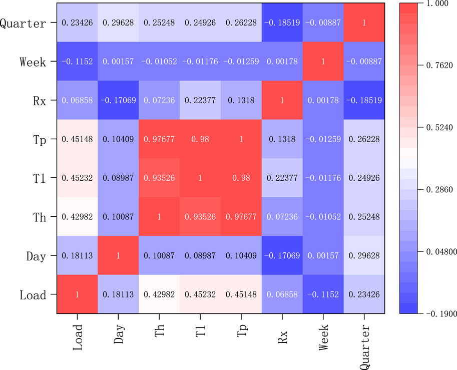
Figure 6. Heat map for correlation analysis.
For experimental comparisons, four model evaluation metrics are used in the paper, namely, the coefficient of determination (R2), the mean absolute error (MAE), the root mean square error (RMSE), and the mean absolute percentage error (MAPE) (Li et al., 2023), as follows:x.
1) R2:
2) MAE:
3) RMSE:
4) MAPE:
Where n denotes the number of predictions, yi'' denotes the predicted value, yi denotes the actual value, and yi'' denotes the average of the true values.
The evaluation indexes of the load forecasting model under different features are shown in Table 1, where the feature terms indicate the features added to the basic features. From Table 1, it can be seen that the R2 of adding weekly features to the basic features is 0.96, the MAE is 0.023 and the RMSE is 0.029 as compared to the load prediction error under other features. Finally, the load, daily maximum temperature, daily minimum date and day of the week were selected as input features for the model.
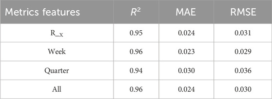
Table 1. Evaluation indicators after adding different characteristics.
As Figure 7 shows the original load waveform, Figure 8 shows the waveform after empirical modal decomposition. Where IMF1 to IMF4 are the decomposed eigenmode functions and IMF5 is the residual quantity.
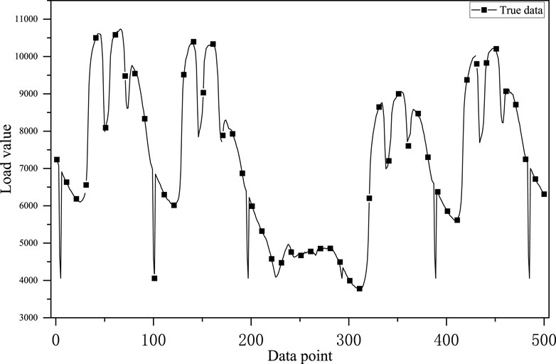
Figure 7. Raw load waveform.
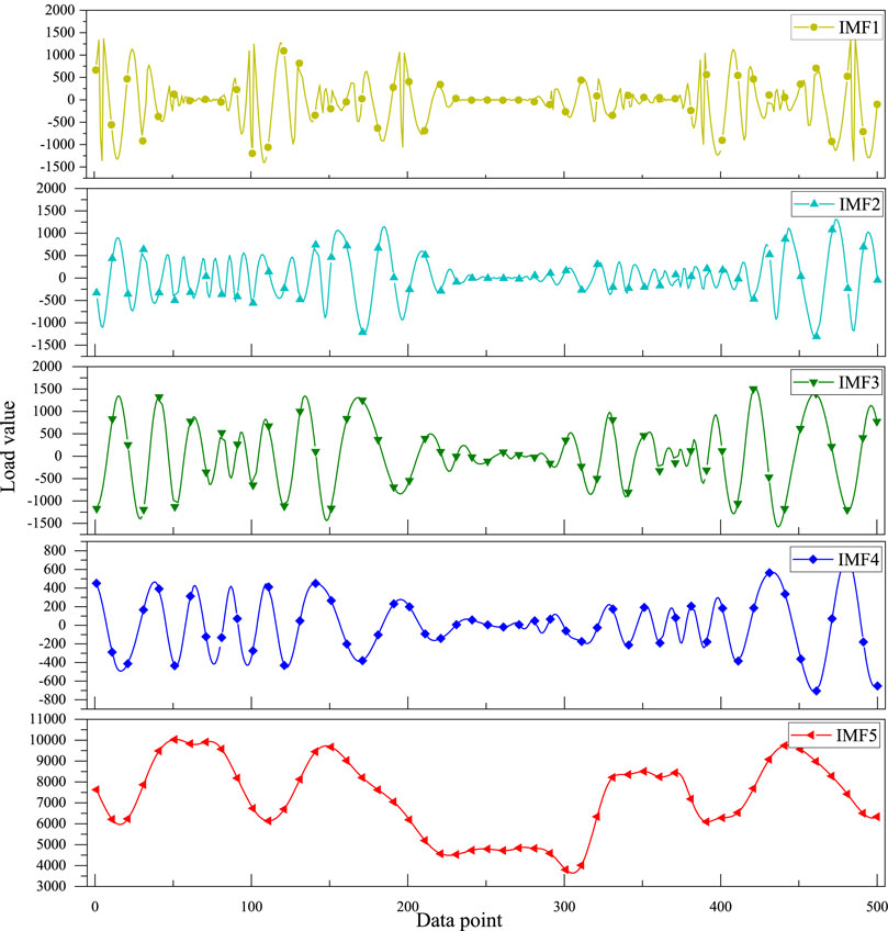
Figure 8. EMD decomposition.
The final prediction results are shown in Figure 9, where the red line indicates the curve predicted by this model, which is closest to the true value.
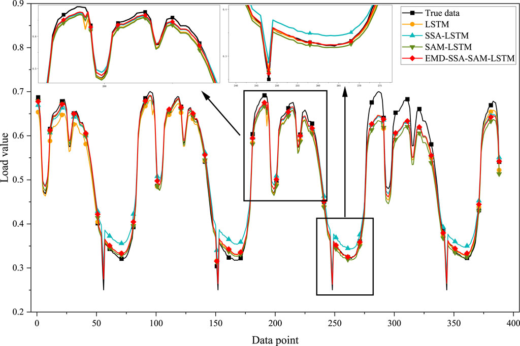
Figure 9. Comparison of load forecast results.
As shown in Table 2 for the evaluation metrics of the different models, it can be seen that the EMD-SSA-SAM-LSTM method has an R2 of 0.98, an MAE of 0.015, an RMSE of 0.019, and a MAPE of 2.04%. There is a maximum coefficient of determination and minimum error. It is verified that the model can improve the load forecasting accuracy.
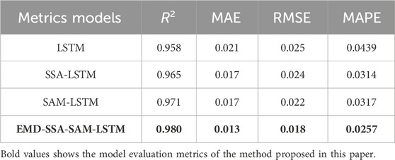
Table 2. Model evaluation indicators.
In this paper, a load forecasting model combining the EMD method, SSA, and LSTM neural network is proposed to improve short-term load forecasting accuracy. Firstly, EMD is used to separate the base load from the randomly fluctuating load, which reduces the nonlinearity of the load. The large component load data is fed into SAM-LSTM and the small component signals are fed into LSTM. To further improve the load prediction accuracy, a sparrow search algorithm is introduced for SAM-LSTM to optimize the hyperparameters of LSTM. Finally, the large-component signal is combined with the small-component signal to obtain the final prediction result.
This paper verifies the validity of the model using the dataset of Question A of the Ninth Electrotechnical Mathematical Modelling Competition, and the results show that the R2 of the proposed EMD-SSA-SAM-LSTM method is 0.98, the MAE is 0.013, the RMSE is 0.018, and the MAPE is 2.57%. Having maximum R2 and minimum error can improve the load forecasting accuracy. This method also has some shortcomings and cannot consider the reduction of model training time, we will try to research in the direction of reducing the time of model training and prediction in the future.
The datasets presented in this study can be found in online repositories. The names of the repository/repositories and accession number(s) can be found below: https://zhuanlan.zhihu.com/p/150954853.
YZ: Investigation, Methodology, Validation, Writing–original draft, Writing–review and editing. ZS: Data curation, Formal Analysis, Investigation, Methodology, Supervision, Visualization, Writing–review and editing. KG: Data curation, Investigation, Methodology, Supervision, Writing–review and editing. ZW: Data curation, Formal Analysis, Investigation, Supervision, Writing–review and editing. WY: Conceptualization, Data curation, Investigation, Methodology, Writing–review and editing. JZ: Investigation, Methodology, Supervision, Writing–review and editing.
The author(s) declare that financial support was received for the research, authorship, and/or publication of this article. This work was funded by Changde Power Supply Branch of State Grid Hunan Electric Power Co. (SGHNCD00DKIS2400150).
Authors FZ, KG, ZW, and WY were employed by the State Grid Hunan Electric Power Company Limited.
The authors declare that this study received funding from Changde Branch, State Grid Hunan Electric Power Co. The funder had the following involvement in the study: The study design and the decision to submit it for publication.
The remaining authors declare that the research was conducted in the absence of any commercial or financial relationships that could be construed as a potential conflict of interest.
All claims expressed in this article are solely those of the authors and do not necessarily represent those of their affiliated organizations, or those of the publisher, the editors and the reviewers. Any product that may be evaluated in this article, or claim that may be made by its manufacturer, is not guaranteed or endorsed by the publisher.
Bin, Z. (2023). Deep learning integration optimization of electric energy load forecasting and market price based on the ANN–LSTM–transformer method. Front. Energy Res. 11. doi:10.3389/fenrg.2023.1292204
Chapagain, K., and Kittipiyakul, P. (2018) “Short-term electricity load forecasting for Thailand,” in 15th international conference on electrical engineering/electronics, computer, telecommunications and information technology (ECTI-CON), 521–524. doi:10.1109/ECTICon.2018.8619930
Gan, D., Wang, Y., Zhang, N., and Zhu, W. (2017). Enhancing short-term probabilistic residential load forecasting with quantile long–short term memory. J. Eng. 2017 (14), 2622–2627. doi:10.1049/joe.2017.0833
Guili, D., Gaoyang, Y., Zongyao, W., Bing, K., Zhihao, X., Xingwang, Z., et al. (2023). Adaptive SPP–CNN–LSTM–ATT wind farm cluster short-term power prediction model based on transitional weather classification. Front. Energy Res. 11. doi:10.3389/fenrg.2023.1253712
Kang, T., Lim, D. Y., Tayara, H., and Chong, K. T. (2020). Forecasting of power demands using deep learning. Appl. Sci. 10 (20), 7241. doi:10.3390/app10207241
Kong, W., Dong, Z. Y., Hill, D. J., Luo, F., and Xu, Y. (2018). Short-term residential load forecasting based on resident behaviour learning. IEEE Trans. Power Syst. 33 (1), 1087–1088. doi:10.1109/TPWRS.2017.2688178
Lee, Y., Tay, K., and Choy, Y. (2018). Forecasting electricity consumption using time series model. Int. J. Eng. Technol. 7 (4.30), 218–223. doi:10.14419/ijet.v7i4.30.22124
Li, Y., Zhao, Y., Wu, L., and Zeng, Z. (2023) Artificial intelligence enabled computational methods for smart grid forecast and dispatch 14. Springer Nature.
Nuo, C., Peng, Z., Xiaofei, R., and Zhenshan, Z. (2023). Electric vehicle charging load prediction based on variational mode decomposition and Prophet-LSTM. Front. Energy Res. 11. doi:10.3389/fenrg.2023.1297849
Rosnalini, M., Bahtiar, J., and Chong, S. Y. (2019). Forecasting of electricity consumption and supply for Campus University using time series models. Int. J. Sup. Chain. Mgt 8 (5), 467–472. doi:10.3390/app10207241
Tang, J., Xu, L., Wu, X., and Chen, K. (2024). A short-term forecasting method for ionospheric TEC combining local attention mechanism and LSTM model. IEEE Geoscience Remote Sens. Lett. 21, 1–5. doi:10.1109/LGRS.2024.3373457
Torres, J. F., Hadjout, D., Sebaa, A., Martínez-Álvarez, F., and Troncoso, A. (2021). Deep learning for time series forecasting: a survey. Big Data 9 (1), 3–21. doi:10.1089/big.2020.0159
Vaswani, A., Shazeer, N., Parmar, N., Uszkoreit, J., Jones, L., Gomez, A. N., et al. (2017). “Attention is all you need,” in Proc. 31st Int. Conf. Adv. Neural Inf. Process. Syst., 6000–6010.
Wu, X., Zhifang, S., Xinhao, F., and Yang, L. (2023). Short-term wind power prediction based on anomalous data cleaning and optimized LSTM network. Front. Energy Res. 11. doi:10.3389/fenrg.2023.1268494
Xiao, H., Gan, H., Yang, P., Li, L., Li, D., Hao, Q., et al. (2024a). Robust submodule fault management in modular multilevel converters with nearest level modulation for uninterrupted power transmission. IEEE Trans. Power Deliv. 39, 931–946. doi:10.1109/TPWRD.2023.3343693
Xiao, H., He, H., Zhang, L., and Liu, T. (2024b). Adaptive grid-synchronization based grid-forming control for voltage source converters. IEEE Trans. Power Syst. 39, 4763–4766. doi:10.1109/TPWRS.2023.3338967
Keywords: short-term power load forecasting, modal decomposition, long short-term memory, self-attention mechanism, hyperparameter optimisation, sparrow search algorithm
Citation: Zhou Y, Su Z, Gao K, Wang Z, Ye W and Zeng J (2024) A short-term electricity load forecasting method integrating empirical modal decomposition with SAM-LSTM. Front. Energy Res. 12:1423692. doi: 10.3389/fenrg.2024.1423692
Received: 26 April 2024; Accepted: 30 May 2024;
Published: 17 June 2024.
Edited by:
Jinpeng Tian, Hong Kong Polytechnic University, Hong Kong SAR, ChinaCopyright © 2024 Zhou, Su, Gao, Wang, Ye and Zeng. This is an open-access article distributed under the terms of the Creative Commons Attribution License (CC BY). The use, distribution or reproduction in other forums is permitted, provided the original author(s) and the copyright owner(s) are credited and that the original publication in this journal is cited, in accordance with accepted academic practice. No use, distribution or reproduction is permitted which does not comply with these terms.
*Correspondence: Zhiyin Su, bTIyMDgwODAwMDE0QHN0dS5odXQuZWR1LmNu
Disclaimer: All claims expressed in this article are solely those of the authors and do not necessarily represent those of their affiliated organizations, or those of the publisher, the editors and the reviewers. Any product that may be evaluated in this article or claim that may be made by its manufacturer is not guaranteed or endorsed by the publisher.
Research integrity at Frontiers
Learn more about the work of our research integrity team to safeguard the quality of each article we publish.