General calculation method of power boundary of multiport power electronic transformer

In the multiport power electronic transformer (MPET), cascaded H-bridge (CHB) converters form the medium voltage AC port, while multiple low voltage DC ports are constructed by paralleling dual active bridge (DAB) converters into clusters. Uneven power distribution among these ports leads to power imbalances, risking over modulation in CHB converters with high power generation or load power. This study proposes a general calculation method (GCM) for determining the power boundary of MPETs, enabling the adjustment of reference power for each DC port to prevent over modulation. The GCM is designed to handle scenarios with multiple simultaneous power flow directions. The effectiveness of the GCM is verified by DC port power boundary simulation results of two independent DC bus structure multiport power electronic transformers. The proposed method provides a straightforward approach to calculating power boundary for MPETs with multiple power flow directions, ensuring efficient power management.

1 Introduction

Multiport power electronic transformer (MPET) provides a competitive solution for the networking of hybrid AC/DC distribution systems due to its compatibility and advanced functionalities (Kolar and Ortiz, 2014; Liserre et al., 2016; Saleh et al., 2019; Ruiz et al., 2020; Li et al., 2021). Multilevel converters, typically the cascaded H-bridge (CHB) converters, are adopted to form the medium voltage AC port for absorbing the active power from AC grid (Huber and Kolar, 2014; Briz et al., 2016; Huang, 2016). With the massive growth of distributed generation (DG), e.g. photovoltaic (PV) generation, and DC loads, e.g. electric vehicle (EV) charging stations, in the distribution network, the low voltage DC (LVDC) ports of the MPET are much more in need. Since the nominal voltage of DGs and DC loads are different, MPET with multiple LVDC ports is significantly necessary and they provide interfaces with multiple voltage levels and power levels (Huber and Kolar, 2019).

Isolated bidirectional DC-DC converters, such as dual active bridge (DAB) converters, can be adopted in MPET to construct multiple LVDC ports (Huang et al., 2011; Zhao et al., 2015; Wang et al., 2016; Costa et al., 2017; Zhao et al., 2018). The input terminals of DABs are directly connected to the DC rails of front-end CHBs. Without adding any additional converters, multiple low voltage DC ports can be constructed by paralleling the output terminals of DABs into multiple clusters (Jia et al., 2019). Therefore, the independent DC bus structure multiport power electronic transformer (IDBS-MPET) can be constructed. There are various parallel connection patterns of DAB output terminals. In detail, a LVDC port can be formed by parallel connection of DABs from a single phase (e.g. Port 2), or two phases (e.g. Port 6), or three phases (e.g. Port 1). The phase mentioned in this paper refers to the AC grid phase a, b or c. Therefore, DGs or DC loads of a LVDC port will be distributed in three phases, evenly or unevenly.

When the power of low voltage DC ports is uneven, power imbalance problem will arise. The front-end CHB converters in the LVDC ports with high power generation or load power will face the risk of over modulation. The power imbalance problem can be further classified into two categories: 1) the interbridge power imbalance, which happens when each bridge in the same phase generates a different amount of power; and 2) the interphase power imbalance, which occurs when each phase generates a different amount of power (Yu et al., 2016). Typically, the interbridge power balance problem lies in the situation of single phase CHB based PV generation system. In (Zhang and Sun, 2019), in order to solve the overmodulation problem when the battery unit is generating PWM voltage with fundamental voltage opposite to that of PV cells, a modified power management scheme is developed where the output power of PV arrays is slightly reduced by an online adjustment scheme, while the output power of the system to grid maintains the same. In (Xue and He, 2023), a flexible power control strategy is proposed to extend the operating range of the PV battery hybrid CHB converter. The injected power of the battery module is controlled adaptively according to the maximum modulation index of all PV modules.

The essence of the interphase power imbalance problem lies in the delivery of three-phase balanced currents to the grid, with unbalanced power in each phase. One efficient way to solve the interphase power imbalance problem of three-phase CHB converters is to inject a zero sequence voltage into the converter output voltages (Yu et al., 2016). With the ZSV injection, the phase of higher power will generate higher output voltage. However, the relationship between the converter phase voltages and the ZSV is nonlinear. Considering the allocation of modulate voltage in each phase, the H-bridge (HB) with highest risk of over modulation cannot be easily determined. The multiple power flow directions of LVDC ports further increased the complexity of the analysis of over modulation situations. As far as the author knows, there is still lack of calculation method of power boundary of three phase MPET. It has significant implications to calculate the power boundary of MPET for its stable operation. The reference power of each LVDC port can be adjusted according to the power boundary to avoiding over modulation.

The main technical contributions of this paper are summarized as follows:

1) The general calculation method (GCM) of power boundary of MPET is proposed. The GCM of power boundary can be applied to the situation where multiple ports have multiple power flow directions simultaneously.

2) The universal expressions for calculating power boundaries have been derived. The expressions can be applied to calculate the power boundary of MPET with any amounts of CHBs and any amounts of LVDC ports.

The rest of this article is organized as follows. Section 2 introduces the topology configuration and makes power imbalance analysis of IDBS-MPET. In Section 3, the modulation ratio calculation method of IDBS-MPET is proposed. In Section 4, analysis of the non-linear characteristics of IDBS-MPET port power boundary analytical expressions and the feasibility of approximate solutions are given. In Section 5, generalized modulation index expressions for the H-bridges in the IDBS-MPET containing three basic DC ports are given. In Section 6, GCM of power boundary of IDBS-MPET is proposed and the universal expressions for calculating power boundaries has been derived. In Section 7, the effectiveness of the GCM of power boundary is verified by simulation results of two IDBS-MPETs. Finally, the conclusion is drawn in Section 8.

2 Topology configuration and power imbalance analysis of IDBS-MPET

2.1 Topology configuration of IDBS-MPET

Based on the connection patterns of DAB output terminals, three basic structures of LVDC ports are established. All kinds of IDBS-MPET can be derived from the combination of the three basic structures (Li et al., 2024). They are the single-phase-connection port (S-Port), the double-cross-phase-connection port (D-Port), and the triple-cross-phase-connection port (T-Port).

The S-Port consists of n_s1 DABs from phase k. As shown in Figure 1, Port 2, Port 3, Port 4, Port 5 and Port 8 belong to the kind of S-Port. The DGs and DC loads connected to the S-Port are distributed in one phase. The D-Port consists of n_d1 DABs from phase k and n_d2 DABs from phase k'. The DGs and DC loads connected to the D-Port are distributed in two phases, evenly or unevenly. If n_d1 = n_d2, the D-Port is denoted as a symmetrical D-Port; otherwise, it is denoted as an asymmetrical D-Port. As shown in Figure 1, Port 6 and Port 7 belong to the kind of D-Port and both of them are symmetrical D-Port. The T-Port consists of n_t1 DABs from phase k, n_t2 DABs from phase k' and n_t3 DABs from phase k''. The DGs and DC loads connected to the T-Port are distributed in three phases, evenly or unevenly. If n_t1 = n_t2 = n_t3, the T-Port is denoted as a symmetrical T-Port; otherwise, it is denoted as an asymmetrical T-Port. As shown in Figure 1, Port1 belongs to the kind of T-Port and it is a symmetrical T-Port.

Figure 1

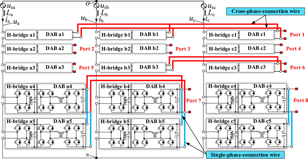
Figure 1. Independent DC bus structure multiport power electronic transformer (IDBS-MPET).

The characteristics of the IDBS-MPET topology are as follows:

(1) Low hardware cost. Multiple DC ports can be constructed without the need for additional DC/DC converters, demonstrating a cost-effective approach to system design.

(2) Cross-phase connection method is utilized during the construction of DC ports, enhancing the system’s flexibility and scalability.

(3) Electrical isolation among all the DC ports ensures safety and reliability.

(4) Modular design. All H-bridges and DABs employ identical electrical parameters, facilitating standardized production and maintenance processes.

The grid current and DC capacitor voltage balancing control of CHB (Jia et al., 2019), maximum power point control of PV (Yu et al., 2016), the voltage feedback control of DAB (Zhao et al., 2013), and charging control of EV and ESS (Yan et al., 2020; Abuishmais and Shahroury, 2021) can also be used in the control of IDBS-MPET. For the paralleled DABs, common-duty-ratio control can be used (Shi et al., 2012).

The IDBS-MPET does not require the addition of any extra DC/DC converters to provide DC ports with multiple voltage and power levels for the connection of DGs and DC loads. This is in contrast to the structure of traditional common DC bus power electronic transformers (CDBS-MPET), as illustrated in Figure 2.

Figure 2

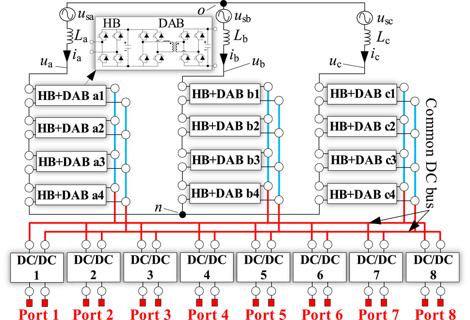
Figure 2. Common DC bus structure multiport power electronic transformer (CDBS-MPET).

Similar to the IDBS-MPET shown in Figure 1, when establishing eight DC ports, the CDBS-MPET requires one DC/DC converter for each port to match the voltage of the DC loads. It has been demonstrated in (Li et al., 2024) that the IDBS-MPET can reduce the number of power semiconductor devices by 40%, significantly lowering costs.

2.2 Essence of power imbalance of IDBS-MPET

Due to the limitations of the total amount of H-bridge converters in each phase, the total amount of LVDC ports and the nominal power of each LVDC port, the LVDC ports in an IDBS-MPET cannot all be constructed as symmetrical T-Ports. The S-Port and D-Port also need to be used. The power imbalance can be divided into two categories: interbridge power imbalance and interphase imbalance (Yu et al., 2016). The interbridge power imbalance will lead to over-modulation of H-bridge converters with larger power. The interphase power imbalance will result in the unbalanced three-phase grid currents.

1) Interphase power imbalance

As shown in Figure 3, the IDBS-MPET contains three DC ports, Port 1, Port 2, and Port 3. Each DC port is formed by parallel connections of four DABs from the same phase. Due to the power balance control employed by the paralleled DABs, the output power from the four DAB converters belonging to the same port is identical, with each contributing one-quarter to the total power of the port. Consequently, within each phase, there is no power discrepancy among the DABs, thereby eliminating issues of imbalance within the phase.

Figure 3

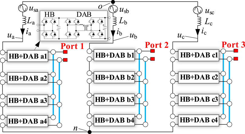
Figure 3. IDBS-MPET with three LVDC ports, which are constructed as single-phase-connection type ports. Port 1, Port 2 and Port 3 are constructed as single-phase-connection type ports.

However, differences in the load power connected to the three DC ports can lead to disparities in power among the three phases, causing interphase power imbalance issues. Such issues of interphase power imbalance can, to a certain extent, be mitigated through the injection of zero sequence voltage, ensuring that the three-phase grid currents of the IDBS-MPET remain symmetrical. When the degree of interphase power imbalance exceeds the compensatory range of the zero sequence voltage, it could lead to overmodulation.

2) Interbridge power imbalance

As shown in Figure 4, the IDBS-MPET contains four DC ports, Port 1, Port 2, Port 3, and Port 4. The power of them is indicated as P₁, P₂, P₃, and P₄, respectively. Each DC port is formed by the parallel connection of three DABs, originating respectively from phases a, b, and c. The deployment of power balance control among the three paralleled DABs ensures that the output power from the three DAB converters belonging to the same port is identical, with each bearing a third of the port’s total power. Consequently, the power drawn from the three phases by each port is the same, thus preventing issues of interphase power imbalance.

Figure 4

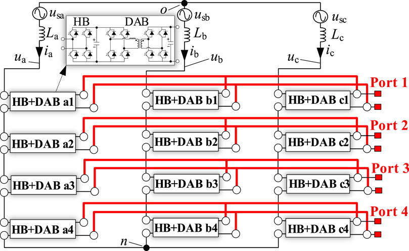
Figure 4. IDBS-MPET with four LVDC ports. Port 1, Port 2, Port 3 and Port 4 are all constructed as symmetrical triple cross-phase-connection type ports.

However, within each phase, such as phase a, the power distributed among H-bridges a1, a2, a3, and a4, i.e., P₁/4, P₂/4, P₃/4, P₄/4, can lead to interbridge power imbalances when the load power of the four DC ports is unequal. Given that H-bridges within the same phase are connected in series and their currents are equal, any imbalance in power among the H-bridges will result in differences in their AC side voltages. The total output voltage of the cascaded H-bridges within a phase must match the grid voltage; hence, excessive disparities in AC side voltages among the H-bridges can lead to overmodulation.

The analysis above delves into the nature of inter-phase and interbridge power imbalances within the IDBS-MPET. Indeed, when the IDBS-MPET encompasses a multitude of ports, the DC ports may be configured in various ways. As demonstrated in Figure 5, Port 1 and Port 2 are constructed using T-Port configurations, whereas Port 3, Port 4, and Port 5 employ S-Port configurations. In such scenarios, the IDBS-MPET is subject to both interphase and interbridge power imbalances, highlighting the complexity and the need for strategic design and control to maintain system balance and efficiency.

Figure 5

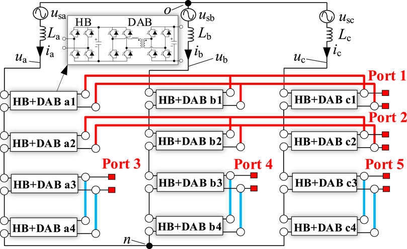
Figure 5. IDBS-MPET with five LVDC ports. Port 1 and Port 2 are constructed as symmetrical triple cross-phase-connection type ports. Port 3, Port 4 and Port 5 are constructed as single-phase-connection type ports.

The IDBS-MPET inverter can be connected directly to a 10 kV medium voltage grid without the line-frequency transformer by reasonably configuring the number of modules, and the voltage and power levels can also be higher. However, interbridge and interphase power imbalance is an inherent problem of the topology, which is difficult to be entirely solved by control strategy alone.

2.3 The necessity of research on the power boundary of IDBS-MPET

It is clear that both interphase and interbridge power imbalances are inherent characteristics of the IDBS-MPET topology. An IDBS-MPET may exhibit solely interphase power imbalance, solely interbridge power imbalance, or both simultaneously. Excessive power imbalance can lead to overmodulation in H-bridge converters, posing a threat to the safe and stable operation of the IDBS-MPET. Therefore, deriving the power boundaries for IDBS-MPET ports and using them to limit the transmission power of the DC ports are fundamental to ensuring the system’s safe and stable operation.

In the IDBS-MPET, the power boundary of port i is influenced by the power states of other ports j (j≠i). Changes in the power state of port j can cause changes in the overall power balance within the IDBS-MPET, both interphase and interbridge. Such imbalances can alter the injection of zero sequence voltage, leading to changes in the phase modulation ratios and the modulation ratios of individual H-bridge modules. Even if the transmission power of port i remains unchanged, changes in the power of other ports j can increase the modulation ratio of the H-bridges included in port i, thereby increasing the risk of overmodulation for these H-bridges. If the transmission power of port i also increases, then the modulation ratio of its included H-bridges will further increase. However, when employing sinusoidal pulse width modulation (SPWM), the modulation ratio of H-bridges cannot exceed 1. Therefore, when any H-bridge within port i reaches a modulation ratio of 1, the transmission power of port i has reached its power boundary. The power boundary of port i dynamically changes with the power state of port j. A significant advantage of the IDBS-MPET is providing DC ports with multiple voltage and power levels for the integration of DGs and DC loads. When an IDBS-MPET has a large number of ports with different power flow directions, some connecting to DGs and others to DC loads, the situation becomes highly complex if any H-bridge within a port experiences overmodulation. The study of power boundaries in such complex scenarios enables better integration of various types of DGs and loads into the IDBS-MPET. Based on the determined power boundaries, effective control strategies can be developed to create more efficient charging solutions for electric vehicles and better consumption strategies for PV integration.

3 Modulation ratio calculation method

As mentioned in Section 2, when the transmission power of a port in the IDBS-MPET reaches its boundary, there must be an H-bridge within the IDBS-MPET with a modulation ratio of 1. Therefore, solving for the modulation ratio of the H-bridge becomes the foundational condition for determining the power boundary of a port. In this section, considering the condition of zero sequence voltage injection, the formula for calculating the modulation ratio of H-bridges within the IDBS-MPET is derived. Given that the application scenario for the IDBS-MPET involves connecting to DGs and supplying power to DC loads, the formula for calculating the H-bridge modulation ratio should ultimately express the power of the DC ports as a variable.

Firstly, the modulation ratios of AC phase voltage m_a, m_b and m_c are calculated. The fundamental component of IDBS-MPET AC phase voltage and AC phase current can be expressed as:

$\left\{\begin{array}{l}{u}_{\mathrm{a}}=U_{\mathrm{p}}\sin \left(\omega t\right)+U_0\sin \left(\omega t+{\theta }_0\right)\\ u_{\mathrm{c}}=U_{\mathrm{p}}\sin \left(\omega t-\frac{2}{3}\pi \right)+U_0\sin \left(\omega t+{\theta }_0\right)\\ u_{\mathrm{b}}=U_{\mathrm{p}}\sin \left(\omega t+\frac{2}{3}\pi \right)+U_0\sin \left(\omega t+{\theta }_0\right)\end{array}\right.(1)$

$\left\{\begin{array}{l}{i}_{\mathrm{a}}=I_{\mathrm{p}}\sin \left(\omega t+{\phi }_{\mathrm{p}}\right)\\ i_{\mathrm{b}}=I_{\mathrm{p}}\sin \left(\omega t-\frac{2}{3}\pi +{\phi }_{\mathrm{p}}\right)\\ i_{\mathrm{c}}=I_{\mathrm{p}}\sin \left(\omega t+\frac{2}{3}\pi +{\phi }_{\mathrm{p}}\right)\end{array}\right.(2)$

where, U_p is the amplitude of positive sequence component of IDBS-MPET AC phase voltage; U₀ and θ₀ is the amplitude and phase angle of zero sequence voltage; I_P is the amplitude of positive sequence component of IDBS-MPET AC phase current; φ_p is the power factor angle; ω is the angular frequency of grid voltage.

As IDBS-MPET mainly deals with active power, the reactive power exchanged with the power grid is very small, which can be considered as φ_p = 0. Then, the three phase power of IDBS-MPET can be calculated from 1 and 2:

$\left\{\begin{array}{l}{P}_{\mathrm{a}}=\frac{1}{2}{U}_{\mathrm{p}}{I}_{\mathrm{p}}+\frac{1}{2}{U}_0{I}_{\mathrm{p}}\cos \left({\theta }_0\right)\\ P_{\mathrm{b}}=\frac{1}{2}{U}_{\mathrm{p}}{I}_{\mathrm{p}}+\frac{1}{2}{U}_0{I}_{\mathrm{p}}\cos \left({\theta }_0+\frac{2}{3}\pi \right)\\ P_{\mathrm{c}}=\frac{1}{2}{U}_{\mathrm{p}}{I}_{\mathrm{p}}+\frac{1}{2}{U}_0{I}_{\mathrm{p}}\cos \left({\theta }_0-\frac{2}{3}\pi \right)\end{array}\right.(3)$

Then, we can get the total power of IDBS-MPET:

$P_{\text{total}}=P_{\mathrm{a}}+P_{\mathrm{b}}+P_{\mathrm{c}}=\frac{3}{2}{U}_{\mathrm{p}}{I}_{\mathrm{p}}(4)$

Based on 1, 3, the U₀ and sine and cosine representation of θ₀ can be obtained as follows:

$\left\{\begin{array}{l}{U}_0=\frac{\sqrt{{\left(3U_p{I}_p-2P_a-4P_b\right)}^2+3{\left(2P_a-U_p{I}_p\right)}^2}}{\sqrt{3}{I}_p}\\ \sin \left({\theta }_0\right)=\frac{3U_p{I}_p-2P_a-4P_b}{\sqrt{{\left(3U_p{I}_p-2P_a-4P_b\right)}^2+3{\left(2P_a-U_p{I}_p\right)}^2}}\\ \cos \left({\theta }_0\right)=\frac{2\sqrt{3}{P}_a-\sqrt{3}{U}_p{I}_p}{\sqrt{{\left(3U_p{I}_p-2P_a-4P_b\right)}^2+3{\left(2P_a-U_p{I}_p\right)}^2}}\end{array}\right.(5)$

According to the basic properties of trigonometric function, for any real number A, B and any angle α, β, the amplitude M_Amp of Asin(α)+Bsin(β) is:

$M_{\text{Amp}}=\sqrt{A^2+B^2+2AB\cos \left(\alpha -\beta \right)}(6)$

Based on 1, 4, 5 and 6, the amplitudes of u_a, u_b, u_c can be expressed as follows:

$\left\{\begin{array}{l}{u}_{am}=\frac{2}{\sqrt{3}{I}_p}\sqrt{3P_a^2+{\left(P_b-P_c\right)}^2}\\ u_{bm}=\frac{2}{\sqrt{3}{I}_p}\sqrt{3P_b^2+{\left(P_a-P_c\right)}^2}\\ u_{cm}=\frac{2}{\sqrt{3}{I}_p}\sqrt{3P_c^2+{\left(P_a-P_b\right)}^2}\end{array}\right.(7)$

Then, the modulation ratios of AC phase voltage can be calculated as:

$\left\{\begin{array}{l}{m}_a=\frac{u_{am}}{N{u}_{dc}}=\frac{\sqrt{3}{U}_p}{N{u}_{dc}}\frac{\sqrt{3P_a^2+{\left(P_b-P_c\right)}^2}}{P_a+P_b+P_c}\\ m_b=\frac{u_{bm}}{N{u}_{dc}}=\frac{\sqrt{3}{U}_p}{N{u}_{dc}}\frac{\sqrt{3P_b^2+{\left(P_a-P_c\right)}^2}}{P_a+P_b+P_c}\\ m_c=\frac{u_{cm}}{N{u}_{dc}}=\frac{\sqrt{3}{U}_p}{N{u}_{dc}}\frac{\sqrt{3P_c^2+{\left(P_a-P_b\right)}^2}}{P_a+P_b+P_c}\end{array}\right.(8)$

where u_dc is the DC voltage of H-bridge converters; N is the amount of H-bridge converters in each phase.

Futher, the equation (8) can be rewitten into a general form as:

$m_k=\frac{u_{km}}{N{u}_{dc}}=\frac{\sqrt{3}{U}_p}{N{u}_{dc}}\frac{\sqrt{3P_k^2+{\left(P_{k^{\prime }}-P_{k^{″}}\right)}^2}}{P_k+P_{k^{\prime }}+P_{k^{″}}}(9)$

Secondly, the H-bridge modulation ratio m_kjn is calculated. In order to calculate m_kjn, the allocation of u_k on H-bridge kjn must be determined. As shown in Figure 6, since the AC current of all H-bridges in phase k are the same, the allocation ratio of u_k on each H-bridge is the ratio of their output power (Wang et al., 2020):

$\frac{u_{\text{ac},{kj}_n,\mathrm{m}}}{\left|P_{\mathrm{H},{kj}_n}\right|}=\frac{u_{k\mathrm{m}}}{\left|P_k\right|}(10)$

where u_ac,kjn is the fundamental component of H-bridge kj_n AC voltage; u_ac,kjn,m is the amplitude of u_ac,kjn; P_H,kjn is the output power of H-bridge kj_n. It is noted that (10) is valid under the condition that P_H,kjn and P_k are all positive. If H-bridge kj_n is absorbing power from the next stage, P_H,kjn will be negative. Considering that P_k may also be positive or negative, the allocation ratio of u_c,F can be expressed as:

$\frac{u_{\text{ac},{kj}_n,\mathrm{m}}}{\left|P_{\mathrm{H},{kj}_n}\right|}=\frac{u_{k\mathrm{m}}}{\left|P_k\right|}(11)$

Figure 6

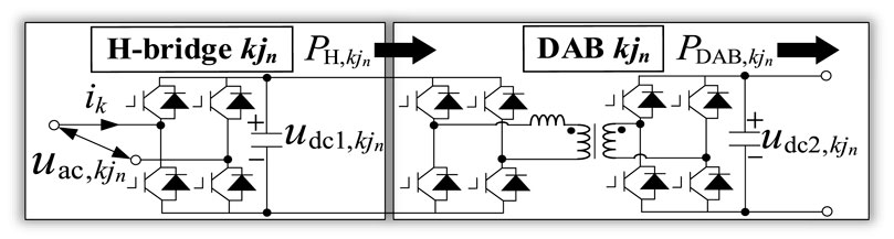
Figure 6. Structure of H-bridge and DAB.

Moreover, m_kjn can be calculated out from (10):

$m_{k{j}_n}=\frac{u_{\text{ac},{kj}_n,\mathrm{m}}}{u_{\text{dc}1,k{j}_n}}=\frac{u_{\text{ac},{kj}_n,\mathrm{m}}}{u_{k\mathrm{m}}}\frac{u_{k\mathrm{m}}}{u_{\text{dc}1,k{j}_n}}=\left|\frac{P_{\mathrm{H},k{j}_n}}{P_k}\right|\frac{u_{k\mathrm{m}}}{u_{\text{dc}1,k{j}_n}}(12)$

where u_dc1,kjn is the DC voltage of H-bridge kj_n.

Ignoring the differences in efficiency among H-bridge converters and the differences in efficiency among DAB converters, (12) can be expressed as:

$m_{k{j}_n}=\left|\frac{P_{\text{DAB},k{j}_n}}{P_k}\right|\frac{u_{k\mathrm{m}}}{u_{\text{dc}1,k{j}_n}}(13)$

where P_DAB,kjn is the output power of DAB kj_n.

As mentioned before in this section, u_dc is the DC voltage of H-bridge converters. Thus, (13) can be finally expressed as:

$m_{k{j}_n}=\left|\frac{P_{\text{DAB},k{j}_n}}{P_k}\right|\frac{u_{k\mathrm{m}}}{u_{\text{dc}}}(14)$

Generally, power balance control is applied on the parallel connected DABs. If Port j consists of n_j DABs and its output power is P_Lj, the output power of each DAB will be P_Lj/n_j in steady state. Thus, the P_DAB,kjn can be expressed as:

$P_{\text{DAB},k{j}_n}=\frac{P_{\mathrm{L}j}}{n_j}(15)$

Ultimately, based on equations 9 and 15, 14 expresses the modulation ratio of the H-bridge as a function of the DC port’s power:

$m_{k{j}_n}={\alpha }_{k{j}_n}N{m}_k(16)$

where

${\alpha }_{k{j}_n}=\frac{1}{n_j}\left|\frac{P_{Lj}}{P_k}\right|(17)$

4 Analysis of the non-linear characteristics of IDBS-MPET port power boundary analytical expressions and the feasibility of approximate solutions

This section comprises two parts. The first part illustrates the nonlinear characteristics of the power boundary expression of an IDBS-MPET with four ports, using it as an example. In the second part, the feasibility of approximating the power boundary through graphical representation of the expression is analyzed.

4.1 Non-linear characteristics of port power analytical expressions

In this paper, the direction of power flow in the IDBS-MPET is defined as follows: when power flows from the grid to the DC port, it is termed positive power, and the value is positive; when power flows from the DC port to the grid, it is termed negative power, and the value is negative. Additionally, the definition of power boundary is divided into upper boundary and lower boundary, where the upper boundary represents the maximum allowable power flow of the DC port, and the lower boundary represents the minimum allowable power flow of the DC port.

The general calculation method of power boundaries will be elaborated in Section 6 of this paper. In this section, we use the four ports IDBS-MPET shown in Figure 7 as an example. Based on the modulation ratio formula derived in Section 3, we analyze the nonlinear characteristics of the power boundary analytical expression of Port 1.

Figure 7

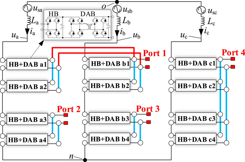
Figure 7. IDBS-MPET with four LVDC ports. Port 1 is constructed as symmetrical double cross-phase-connection type port. Port 2, Port 3, and Port 4 are constructed as single-phase-connection type ports.

In the IDBS-MPET shown in Figure 7, apart from Port 1 being sought, the current powers of other ports (Port 2, Port 3, and Port 4) as well as the electrical parameters of the IDBS-MPET are shown in Tables 1, 2, respectively. From the analysis in Part C of Section 2, it is evident that when any modulation ratio of the H-bridges within the IDBS-MPET equals 1, the calculated power of Port 1, namely the power boundary of Port 1, is obtained.

Table 1

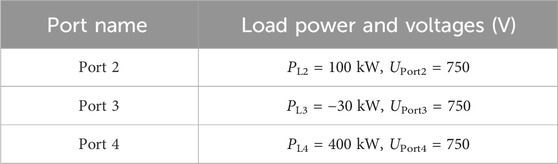
Table 1. Load Power and Voltages of the Port 2, Port 3 and Port 4 in the IDBS-MPET shown in Figure 7.

Table 2

Table 2. Circuit parameters of the IDBS-MPET in Figure 7.

Based on the structure of the IDBS-MPET in Figure 7, all H-bridges can be categorized into three types: the first type comprises H-bridges contained within the Port 1 itself, namely H-bridges a1, a2, b1, and b2; the second type comprises H-bridges within the same phases (phase a and phase b) as the Port 1 but not contained within the Port 1 itself, namely H-bridges a3, a4, b3, and b4; the third type comprises H-bridges within phase other than the one containing the Port 1, namely H-bridges c1, c2, c3, and c4.

Let the current power of Port 1 be P_L1, Port 2 be P_L2, Port 3 be P_L3, and Port 4 be P_L4. Each port employs power balance control for its included DABs, thus the power of each DAB is 1/n_j of the total port power, where n_j represents the number of DABs included in port j. Consequently, the three-phase power of the IDBS-MPET can be represented using P_L1 and P_L2 as follows:

$\left\{\begin{array}{l}{P}_a=\frac{1}{2}{P}_{L1}+P_{L2}\\ P_b=\frac{1}{2}{P}_{L1}+P_{L3}\\ P_c=P_{L4}\end{array}\right.(18)$

By simultaneously solving equations (8) and, (16), and (18), the calculation formulas for the aforementioned three types of H-bridge modulation ratios can be derived. Setting these modulation ratios to 1 allows us to determine their respective constraints on the power boundary of Port 1. Next, we analyze the piecewise linear characteristics of the power boundary expression of Port 1 under the constraints of these three types of H-bridge modulation ratios. Here, we define the rated modulation ratio m_N to establish the relationship between U_p, u_dc, and N, denoted as:

$m_N=\frac{U_p}{N{u}_{dc}}(19)$

(1) Modulation ratios of the first type H-bridges, namely, the H-bridges contained within the Port 1 itself

The modulation ratios of H-bridge a1 and H-bridge a2, denoted as m_a1 and m_a2, are represented as shown in equation (20), while the modulation ratios of H-bridge b1 and H-bridge b2, denoted as m_b1 and m_b2, are expressed as shown in equation (21).:

$\begin{array}{l}{m}_{a1}=m_{a2}=\\ \frac{\sqrt{P_{L1}^2+\left(3P_{L2}+P_{L3}-P_{L4}\right)P_{L1}+3P_{L2}^2+{\left(P_{L3}-P_{L4}\right)}^2}}{\left|\frac{2}{\sqrt{3}N{m}_N}{P}_{L1}+\frac{4P_{L2}\left(P_{L2}+P_{L3}+P_{L4}\right)}{\sqrt{3}N{m}_N}\frac{1}{P_{L1}}+\frac{2\left(3P_{L2}+P_{L3}+P_{L4}\right)}{\sqrt{3}N{m}_N}\right|}\end{array}(20)$

$\begin{array}{l}{m}_{b1}=m_{b2}=\\ \frac{\sqrt{P_{L1}^2+\left(3P_{L3}+P_{L2}-P_{L4}\right)P_{L1}+3P_{L3}^2+{\left(P_{L2}-P_{L4}\right)}^2}}{\left|\frac{2}{\sqrt{3}N{m}_N}{P}_{L1}+\frac{4P_{L3}\left(P_{L2}+P_{L3}+P_{L4}\right)}{\sqrt{3}N{m}_N}\frac{1}{P_{L1}}+\frac{2\left(P_{L2}+3P_{L3}+P_{L4}\right)}{\sqrt{3}N{m}_N}\right|}\end{array}(21)$

From equations (20) and (21), it can be observed that the numerator of the modulation ratio expression for the H-bridges contained within the Port 1 itself can both be represented as the square root of a quadratic equation with P_L1 as the variable:

$f_1\left(P_{L1}\right)=\sqrt{{\lambda }_1{P}_{L1}^2+{\lambda }_2{P}_{L1}+{\lambda }_3}(22)$

It should be noted that λ₁ is a coefficient associated with the number of H-bridges distributed in phases a and b with respect to Port 1, hence λ₁ > 0; λ₂ is a coefficient related to the powers of the remaining ports, thus λ₂ may be greater than 0 or less than 0; λ₃ is the sum of two square terms, thus λ₃ ≥ 0. Additionally, the function f₁(P_L1) is obtained by substituting equation (18) into equation (8), hence the overall value under the square root in f₁(P_L1) must be greater than or equal to 0.

The denominators of equations (20) and (21) can both be expressed as the absolute value squared function with P_L1 power as the variable:

$f_2\left(P_{L1}\right)=\left|{\lambda }_4{P}_{L1}+{\lambda }_5\frac{1}{P_{L1}}+{\lambda }_6\right|(23)$

It should be noted that λ₄ is a coefficient associated with the number of H-bridges cascaded in each phase, N, and the rated modulation ratio, m_N, thus λ₄ > 0; λ₅ and λ₆ are coefficients related to the powers of the remaining ports, hence λ₅ and λ₆ may be greater than 0 or less than 0.

Therefore, the modulation ratio of H-bridges contained within Port 1 itself can be expressed in a general form as:

$m_{k{j}_n}=\frac{f_1\left(P_{L1}\right)}{f_2\left(P_{L1}\right)}=\frac{\sqrt{{\lambda }_1{P}_{L1}^2+{\lambda }_2{P}_{L1}+{\lambda }_3}}{\left|{\lambda }_4{P}_{L1}+{\lambda }_5\frac{1}{P_{L1}}+{\lambda }_6\right|}(24)$

For the H-bridges contained within Port 1 itself, except for λ₁ and λ₄, the other coefficients are not the same.

Based on equation (24) and the parameters from Tables 1, 2, the graphs of the numerator and denominator functions of the modulation ratios m_a1 and m_a2 for H-bridges a1 and a2 can be plotted as shown in Figure 8, while the graphs of the numerator and denominator functions of the modulation ratios m_b1 and m_b2 for H-bridges b1 and b2 can be plotted as shown in Figure 9. Since the H-bridges cannot be over-modulated, i.e., m_kjn < 1, the feasible solution region for P_L1 in Figures 8, 9 corresponds to the part where f₂(P_L1) > f₁(P_L1), highlighted with black diagonal lines. It is noteworthy that the form of the denominator function f₂(P_L1) in Figure 8 is different from that in Figure 9, due to the coefficient λ₅ > 0 in the modulation ratio expressions for m_a1 and m_a2 of H-bridges a1 and a2, while the coefficient λ₅ < 0 in the modulation ratio expressions for m_b1 and m_b2 of H-bridges b1 and b2.

Figure 8

Figure 8. The graph of the numerator function f₁(P_L1) for the modulation ratio expression of H-bridges a1 and a2, the graph of the numerator approximation function f_1,linear (P_L1), and the graph of the denominator function f₂(P_L1).

Figure 9

Figure 9. The graph of the numerator function f₁(P_L1) for the modulation ratio expression of H-bridges b1 and b2, the graph of the numerator approximation function f_1,linear (P_L1), and the graph of the denominator function f₂(P_L1).

Setting m_kjn = 1 in equation (24), the constraint conditions of the H-bridges contained within Port 1 itself on the power boundary of Port 1 can be determined as:

$\begin{array}{l}{P}_{L1}^4\left({\lambda }_1-{\lambda }_4^2\right)+P_{L1}^3\left({\lambda }_2-2{\lambda }_4{\lambda }_6\right)+P_{L1}^2\left({\lambda }_3-2{\lambda }_4{\lambda }_5-{\lambda }_6^2\right)-\\ 2P_{L1}{\lambda }_5{\lambda }_6-{\lambda }_5^2=0\end{array}(25)$

From equation (25), it can be observed that this constraint condition forms a fourth-order polynomial equation with respect to P_L1, exhibiting nonlinear characteristics.

(2) Modulation ratios of the second type H-bridges, namely, the H-bridges within the same phase as the Port 1 but not contained within the Port 1 itself

The modulation ratios of H-bridges a3 and a4, denoted as m_a3 and m_a4, are expressed as shown in equation (26), while the modulation ratios of H-bridges b3 and b4, denoted as m_b3 and m_b4, are expressed as shown in equation (27).

$\begin{array}{l}{m}_{a3}=m_{a4}=\\ \frac{\sqrt{P_{L1}^2+\left(3P_{L2}+P_{L3}-P_{L4}\right)P_{L1}+3P_{L2}^2+{\left(P_{L3}-P_{L4}\right)}^2}}{\left|\frac{1}{2\sqrt{3}N{m}_N{P}_{a{j}_n}}{P}_{L1}^2+\frac{3P_{L2}+P_{L3}+P_{L4}}{2\sqrt{3}N{m}_N{P}_{a{j}_n}}{P}_{L1}+\frac{2P_{L2}\left(P_{L2}+P_{L3}+P_{L4}\right)}{2\sqrt{3}N{m}_N{P}_{a{j}_n}}\right|}\end{array}(26)$

where, P_ajn represents the power of H-bridge a3 or a4.

$\begin{array}{l}{m}_{b3}=m_{b4}=\\ \frac{\sqrt{P_{L1}^2+\left(P_{L2}+3P_{L3}-P_{L4}\right)P_{L1}+3P_{L3}^2+{\left(P_{L2}-P_{L4}\right)}^2}}{\left|\frac{1}{2\sqrt{3}N{m}_N{P}_{b{j}_n}}{P}_{L1}^2+\frac{P_{L2}+3P_{L3}+P_{L4}}{2\sqrt{3}N{m}_N{P}_{b{j}_n}}{P}_{L1}+\frac{2P_{L3}\left(P_{L2}+P_{L3}+P_{L4}\right)}{2\sqrt{3}N{m}_N{P}_{b{j}_n}}\right|}\end{array}(27)$

where, P_bjn represents the power of H-bridge b3 or b4.

The denominators of equations (24) and (25) can both be expressed as quadratic functions with Port 1 power as the variable:

$f_3\left(P_{L1}\right)={\lambda }_7{P}_{L1}^2+{\lambda }_8{P}_{L1}+{\lambda }_9(28)$

It should be noted that λ₇ is a coefficient associated with the number of H-bridges cascaded in each phase, N, and the rated modulation ratio, m_N, thus λ₇ > 0; λ₅ and λ₆ are coefficients related to the powers of the remaining ports, hence λ₅ and λ₆ may be greater than 0 or less than 0.

Therefore, the modulation ratio of H-bridges within the same phase as Port 1 but not contained within Port 1 itself can be expressed in a general form:

$m_{k{j}_n}=\frac{f_1\left(P_{L1}\right)}{f_3\left(P_{L1}\right)}=\frac{\sqrt{{\lambda }_1{P}_{L1}^2+{\lambda }_2{P}_{L1}+{\lambda }_3}}{\left|{\lambda }_7{P}_{L1}^2+{\lambda }_8{P}_{L1}+{\lambda }_9\right|}(29)$

Based on equation (29) and the parameters from Tables 1, 2, the graphs of the numerator and denominator functions of the modulation ratios m_a3 and m_a4 for H-bridges a3 and a4 can be plotted as shown in Figure 10, while the graphs of the numerator and denominator functions of the modulation ratios m_b3 and m_b4 for H-bridges b3 and b4 can be plotted as shown in Figure 11. Since the H-bridges cannot be over-modulated, i.e., m_kjn < 1, the feasible solution region for P_L1 in Figure 10 and Figure 11 corresponds to the part where f₃(P_L1) > f₁(P_L1), highlighted with black diagonal lines.

Figure 10

Figure 10. The graph of the numerator function f₁(P_L1) for the modulation ratio expression of H-bridges a3 and a4, the graph of the numerator approximation function f_1,linear (P_L1), and the graph of the denominator function f₃(P_L1).

Figure 11

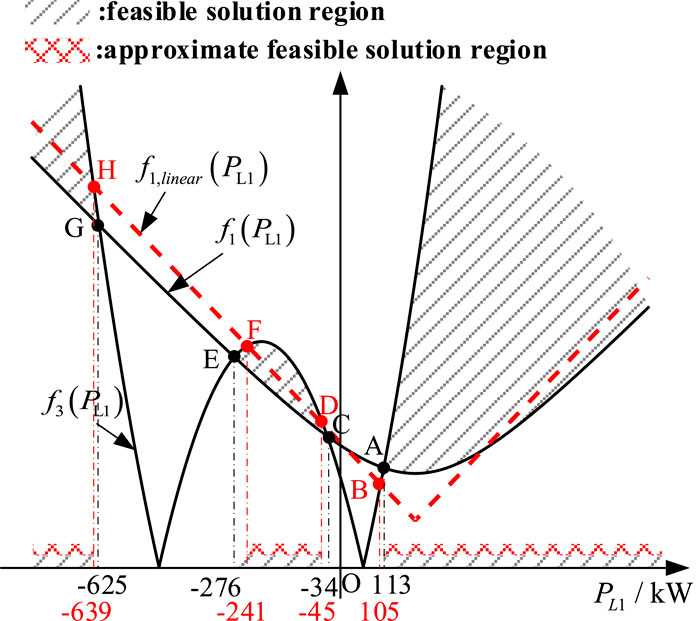
Figure 11. The graph of the numerator function f₁(P_L1) for the modulation ratio expression of H-bridges b3 and b4, the graph of the numerator approximation function f_1,linear (P_L1), and the graph of the denominator function f₃(P_L1).

Setting m_kjn = 1 in equation (29), the constraint conditions of the H-bridges within the same phase as Port 1 but not contained within Port 1 itself on the Port 1 power boundary can be determined as equation (30):

$\begin{array}{l}{P}_L^4{\lambda }_7^2+2P_L^3{\lambda }_7{\lambda }_8+{\lambda }_9^2+P_L^2\left(-{\lambda }_1+{\lambda }_8^2+2{\lambda }_7{\lambda }_9\right)+\\ P_L\left(-{\lambda }_2+2{\lambda }_8{\lambda }_9\right)-{\lambda }_3=0\end{array}(30)$

Similar to equation (25), the constraint condition of equation (30) remains a fourth-order polynomial equation with respect to P_L1, exhibiting nonlinear characteristics.

(3) Modulation ratios of the third type H-bridges, namely, the H-bridges within the phase other than the ones containing the Port 1

The modulation ratios of H-bridges c1, c2, c3, and c4, denoted as m_c1, m_c2, m_c3, and m_c4, are expressed as shown in equation (31):

$\begin{array}{l}{m}_{c1}=m_{c2}=m_{c2}=m_{c2}=\\ \frac{\sqrt{{\left(P_{L2}-P_{L3}\right)}^2+3P_{L4}^2}}{\left|\frac{P_{L4}}{\sqrt{3}N{m}_N{P}_{c{j}_n}}{P}_{L1}+\frac{P_{L4}}{\sqrt{3}N{m}_N{P}_{c{j}_n}}\left(P_{L2}+P_{L3}+P_{L4}\right)\right|}\end{array}(31)$

where, P_cjn represents the power of H-bridge c1, c2, c3, or c4.

From equation (31), it can be observed that the numerator of the modulation ratio expression for H-bridges within phases other than the one containing the port is independent of Port 1 power. The numerator remains represented by f₁(P_L1), where now only the λ₃ term is included:

$f_1\left(P_{L1}\right)=\sqrt{{\lambda }_3}(32)$

The denominator of equation (30) can be expressed as a linear function with Port 1 power as the variable:

$f_4\left(P_{L1}\right)={\lambda }_{10}{P}_{L1}+{\lambda }_{11}(33)$

Therefore, the modulation ratio of H-bridges within phases other than the one containing Port 1 can be expressed in a general form:

$m_{k{j}_n}=\frac{f_1\left(P_{L1}\right)}{f_4\left(P_{L1}\right)}=\frac{\sqrt{{\lambda }_3}}{{\lambda }_{10}{P}_{L1}+{\lambda }_{11}}(34)$

Based on equation (34) and the parameters from Tables 1, 2, the graphs of the numerator and denominator functions of the modulation ratios m_c1, m_c2, m_c3, and m_c4 for H-bridges c1, c2, c3, and c4 can be plotted as shown in Figure 12. Since the H-bridges cannot be over modulated, i.e., m_kjn < 1, the feasible solution region for P_L1 in Figure 12 corresponds to the part where f₄(P_L1) > f₁(P_L1), highlighted with black diagonal lines.

Figure 12

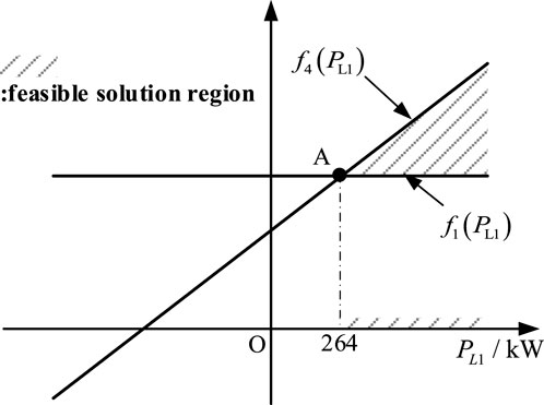
Figure 12. The graph of the numerator function f₁(P_L1) for the modulation ratio expression of H-bridges c1, c2, c3, and c4, and the graph of the denominator function f₄(P_L1).

Setting m_kjn = 1 in equation (34), the constraint conditions of the H-bridges within the phase other than the one containing Port 1 on the Port 1 power boundary can be determined as equation (35):

${\lambda }_{10}{P}_{L1}+{\lambda }_{11}-\sqrt{{\lambda }_3}=0(35)$

The constraint condition of equation (35) on P_L1 is linear.

Through the above analysis, it is evident that the modulation ratio of H-bridges contained within Port 1 itself, the modulation ratio of H-bridges within the same phase as Port 1 but not contained within Port 1 itself, all impose nonlinear constraints on the power boundary of Port 1. Although the modulation ratio of H-bridges within phases other than the one containing Port 1 imposes linear constraints on P_L1, as shown in Figure 12, it only imposes lower boundary constraints on P_L1 without upper boundary constraints.

Since λ₂, λ₃, λ₅, λ₆, λ₇, λ₈, and λ₉ are coefficients related to the powers of the other ports, the solution of P_L1 with respect to the power of any other port obtained from equations (25) and (30) is also nonlinear.

Moreover, directly solving equations (25) and (30) is extremely complex and would exacerbate the computational burden of the controller, making it difficult to quickly analyze the power boundary of Port 1 and posing significant challenges for real-time control of IDBS-MPET.

B. Feasibility analysis of approximating the forward power boundary.

Upon analyzing equations (24) and (29), it can be observed that the complexity of equations (25) and (30) as fourth-order equations arise due to the square root function in the numerator of the H-bridge modulation ratio expression. Therefore, simplifying the determination of power boundaries hinges on approximating the function f₁(P_L1). This paper proposes approximating f₁(P_L1) as the absolute value of a linear function of P_L1, denoted as f_1,linear (P_L1), to achieve an approximate solution to the power boundaries. Let’s take the image of the numerator f₁(P_L1) in the modulation ratio expression of H-bridge a1, a2 as an example to elucidate the feasibility of approximating port power boundaries. Next, we analyze the properties of the function f₁(P_L1) image.

Property 1: The image of f₁(P_L1) is a parabola opening upwards and does not intersect the horizontal axis (P_L1 axis). As shown in Figures 8–11, since the coefficient λ₂ can be positive or negative, the minimum point M₁ $\left(-{\lambda }_2/2{\lambda }_1,\sqrt{{\lambda }_3-{\lambda }_2^2/4{\lambda }_1}\right)$ of the f₁(P_L1) image may be on the left or right side of the vertical axis, as illustrated in Figure 13.

Figure 13

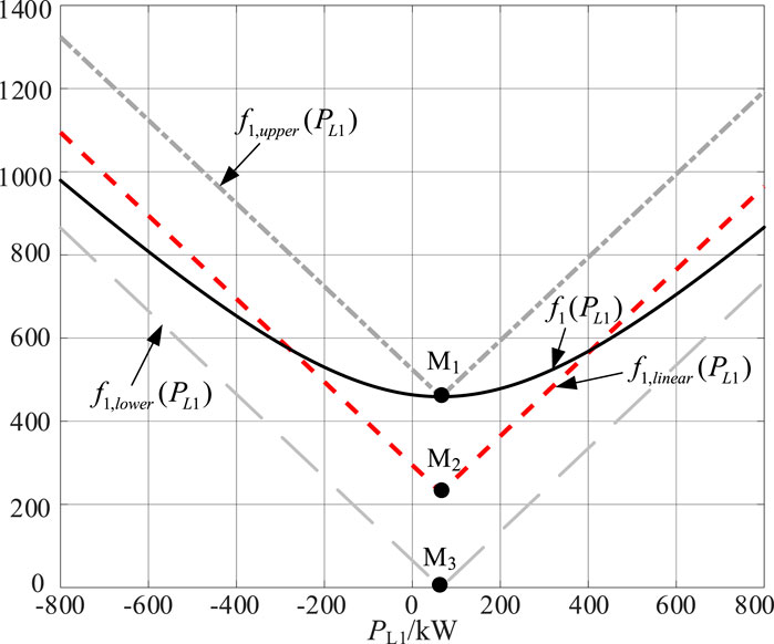
Figure 13. The graph of the numerator function f₁(P_L1) for the modulation ratio, its approximate function f_1,linear (P_L1), its lower boundary function f_1,lower (P_L1), its upper boundary function f_1,upper (P_L1).

Property 2: As P_L1 tends to positive infinity, f₁(P_L1) has an asymptotic line with a slope of $\sqrt{{\lambda }_1}$; as P_L1 tends to negative infinity, f₁(P_L1) has an asymptotic line with a slope of $-\sqrt{{\lambda }_1}$. This property can be obtained by differentiating f₁(P_L1), as shown in equation (36):

$f_1^{\prime }\left(P_{L1}\right)=\left\{\begin{array}{l}{\lambda }_2/2\sqrt{{\lambda }_3},P_{L1}=0\\ \frac{{\lambda }_1+{\lambda }_2/2P_{L1}}{{\left(-1\right)}^{\text{sgn}}\sqrt{{\lambda }_1+{\lambda }_2/\left|P_{L1}\right|+{\lambda }_3/P_{L1}^2}},P_{L1}\ne 0\end{array}\right.(36)$

where sgn = 0 when P_L1 > 0, and sgn = 1 when P_L1 < 0. From equation (36), we can derive the limits of $f_1^{\prime }\left(P_{L1}\right)$ as P_L1 approaches positive infinity and negative infinity, respectively, as follows:

$\left\{\begin{array}{l}\underset{P_{L1}\to +\infty }{\lim }{f}_1^{\prime }\left(P_{L1}\right)=\sqrt{{\lambda }_1}\\ \underset{P_{L1}\to -\infty }{\lim }{f}_1^{\prime }\left(P_{L1}\right)=-\sqrt{{\lambda }_1}\end{array}\right.(37)$

Based on the properties of the f₁(P_L1), we can construct the function f_1,lower using the slopes $\sqrt{{\lambda }_1}$ and $-\sqrt{{\lambda }_1}$ of its asymptotes passing through point M₃ $\left(-{\lambda }_2/2{\lambda }_1,0\right)$:

$f_{1,lower}\left(P_{L1}\right)=\left|\sqrt{{\lambda }_1}{P}_{L1}+{\lambda }_2/2\sqrt{{\lambda }_1}\right|(38)$

Passing through point M₁, which represents the minimum value of f₁(P_L1), we can define the function f_1,upper:

$f_{1,upper}\left(P_{L1}\right)=\left|\sqrt{{\lambda }_1}{P}_{L1}+{\lambda }_2/2\sqrt{{\lambda }_1}\right|+\sqrt{{\lambda }_3-{\lambda }_2^2/4{\lambda }_1}(39)$

The minimum point M₃ of f_1,lower (P_L1) lies below the minimum point M₁ of f₁(P_L1), with a slope equal to that of the asymptote of f₁(P_L1). Thus, f_1,lower (P_L1) can serve as the lower bound of f₁(P_L1), and as |P_L1| tends to infinity, f₁(P_L1) converges to f_1,lower (P_L1). The minimum point M₁ of f_1,upper (P_L1) is the same as that of f₁(P_L1), with a slope identical to the asymptote of f₁(P_L1), indicating that f_1,upper (P_L1) can act as the upper bound of f₁(P_L1).

To reduce the approximation error, this paper proposes approximating function f_1,linear (P_L1) as the midpoint between the upper bound function f_1,upper (P_L1) and the lower bound function f_1,lower (P_L1), i.e., a function passing through point M₂ $\left(-{\lambda }_2/2{\lambda }_1,\sqrt{{\lambda }_3-{\lambda }_2^2/4{\lambda }_1}/2\right)$ with slopes $\sqrt{{\lambda }_1}$ and $-\sqrt{{\lambda }_1}$:

$f_{1,linear}\left(P_{L1}\right)=\left|\sqrt{{\lambda }_1}{P}_{L1}+{\lambda }_2/2\sqrt{{\lambda }_1}\right|+\sqrt{{\lambda }_3-{\lambda }_2^2/4{\lambda }_1}/2(40)$

Function f_1,linear (P_L1) is plotted in Figures 8–11 and indicated by red dashed lines.

Equation (24) is rewritten using equation (40) as follows:

$m_{k{j}_n}=\frac{f_{1,linear}\left(P_{L1}\right)}{f_2\left(P_{L1}\right)}=\left|\frac{\left|\sqrt{{\lambda }_1}{P}_{L1}+{\lambda }_2/2\sqrt{{\lambda }_1}\right|+\sqrt{{\lambda }_3-{\lambda }_2^2/4{\lambda }_1}/2}{{\lambda }_4{P}_{L1}+{\lambda }_5\frac{1}{P_{L1}}+{\lambda }_6}\right|(41)$

Taking point B in Figure 8 as an example, Eq. 41 is transformed into:

$m_{k{j}_n}=\frac{\sqrt{{\lambda }_1}{P}_{L1}+{\lambda }_2/2\sqrt{{\lambda }_1}+\sqrt{{\lambda }_3-{\lambda }_2^2/4{\lambda }_1}/2}{{\lambda }_4{P}_{L1}+{\lambda }_5\frac{1}{P_{L1}}+{\lambda }_6}(42)$

By setting m_kjn = 1 in Eq. 42, the constraints of the H-bridge contained in Port 1 on the power boundary of Port 1 can be determined:

$P_{L1}^2\left(\sqrt{{\lambda }_1}-{\lambda }_4\right)+P_{L1}\left(\frac{{\lambda }_2}{2\sqrt{{\lambda }_1}}+\frac{1}{4}\sqrt{4{\lambda }_3-\frac{{\lambda }_2^2}{{\lambda }_1}}-{\lambda }_6\right)-{\lambda }_5=0(43)$

Comparing with Eq. 25, it is evident that by approximating f₁(P_L1) as f_1,linear (P_L1), the solution to the modulation ratio constraint shifts from a fourth-order equation in P_L1 to a quadratic equation. The roots can be determined by using the quadratic formula.

Figure 14 illustrates the errors between f_1,linear (P_L1) and f₁(P_L1), and it is defined as:

${\epsilon }_1=\frac{f_{1,linear}\left(P_{L1}\right)-f_1\left(P_{L1}\right)}{f_1\left(P_{L1}\right)}(44)$

Figure 14

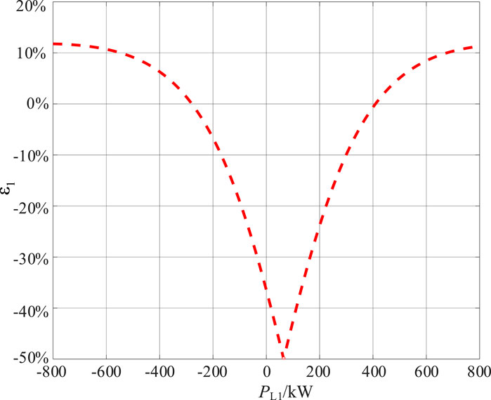
Figure 14. Error between of f₁(P_L1) and its approximate function f_1,linear (P_L1), its lower boundary function f_1,lower (P_L1), its upper boundary function f_1,upper (P_L1).

It can be observed that the maximum error between f_1,linear (P_L1) and f₁(P_L1) occurs at the minimum point of f₁(P_L1), reaching 50%.

5 Generalized modulation index expressions for the H-bridges in the IDBS-MPET containing three basic DC ports

Based on the analysis in Section 4, the power boundary of the DC port is obtained by evaluating the modulation index of any H-bridge within the DC port reaching unity using its modulation index expression. The calculation of the modulation index serves as a prerequisite for determining the power boundary.

However, from the IDBS-MPET diagrams in Figures 1–5, it is evident that the port types are diverse. It would be overly complex to establish specific modulation index expressions for each type of IDBS-MPET port. Hence, we aim to develop a generalized formula for calculating the modulation index. This formula should rely solely on input topological parameters such as the number of cascaded H-bridges and the number of H-bridges included in the DC port under consideration, enabling the utilization of a universal expression for modulation index computation.

Previous literature has identified three fundamental types of DC ports in IDBS-MPET: the S-Ports, the D-Ports (symmetrical and asymmetrical), and the T-Ports (symmetrical and asymmetrical) (Li et al., 2024). Through these three basic types of DC ports, all types of IDBS-MPET can be constructed. By individually deriving the generalized modulation index expressions for each H-bridge within these three basic types of DC ports in IDBS-MPET, a comprehensive universal modulation index calculation formula can be established.

As mentioned in Section Ⅳ, when multiple ports within the IDBS-MPET have inconsistent power flows, the limiting factor for the power boundary of the port under consideration may not necessarily be the modulation index of the H-bridges within that port. It is possible that the modulation index of H-bridges within other ports poses a greater risk of over modulation, thereby restricting the power boundary of the port under consideration. When computing the power boundary of the port under consideration, it is not necessary to calculate the modulation index of all H-bridges within the IDBS-MPET. The proposed universal power boundary calculation method includes a procedure to identify the H-bridge module with the highest risk of over-modulation, significantly reducing computational overhead. This will be discussed in detail in Section Ⅴ.

This section is divided into three parts, each establishing the generalized modulation index expressions for the H-bridges within the three fundamental types of DC ports in IDBS-MPET.

5.1 The generalized modulation index expression for each H-bridge in the IDBS-MPET containing S-Port

It may be as well to take the IDBS-MPET containing the S-Port in phase a as an example to make the derivation of the generalized modulation index, as illustrated in Figure 15. The modulation index derivation process of H-bridges in the IDBS-MPET containing S-Port in phases b or phase c is similar to the following derivation process.

Figure 15

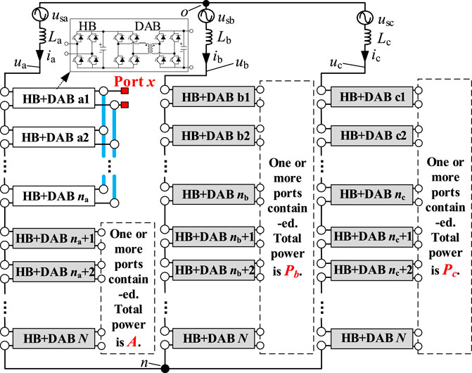
Figure 15. The IDBS-MPET containing S-Port in phase a.

Let the power of Port x be P_Lx; the total output power of DAB except for the one contained in Port x in phase a is denoted as A; the total power in phase b is P_b; and the total power in phase c is P_c. By employing the approximation method outlined in Equation 40, the modulation ratios for phases a, b, and c can be approximated as follows:

$\left\{\begin{array}{l}{m}_a\approx \frac{\sqrt{3}{U}_p}{N{V}_{dc}}\frac{\sqrt{3}\left|P_{Lx}+A\right|+\frac{1}{2}\left|P_b-P_c\right|}{P_{Lx}+A+P_b+P_c}\\ m_b\approx \frac{\sqrt{3}{U}_p}{N{V}_{dc}}\frac{\left|P_{Lx}+A-P_c\right|+\frac{\sqrt{3}}{2}\left|P_b\right|}{P_{Lx}+A+P_b+P_c}\\ m_c\approx \frac{\sqrt{3}{U}_p}{N{V}_{dc}}\frac{\left|P_{Lx}+A-P_b\right|+\frac{\sqrt{3}}{2}\left|P_c\right|}{P_{Lx}+A+P_b+P_c}\end{array}\right.(45)$

Substituting Eq. 45 into Eq. 16, while also taking into account the proportional relationship between the power of each H-bridge and the phase power as depicted in Figure 17, we can derive the general expression for the modulation ratio of each H-bridge as follows:

(1) For the H-bridges contained within the Port x, the generalized calculation formula for the modulation index of the H-bridge itself is as follows:

$m_{ak}=\frac{\left|P_{Lx}+A\right|+\frac{1}{2\sqrt{3}}\left|P_b-P_c\right|}{\frac{n_a}{3N{m}_N}{P}_{Lx}+\frac{A{n}_a\left(A+P_b+P_c\right)}{3N{m}_N}\frac{1}{P_{Lx}}+\frac{n_a}{3N{m}_N}\left(2A+P_b+P_c\right)}(46)$

(2) For the H-bridges in phase a but not contained within the Port x itself, the generalized calculation formula for the modulation index of each H-bridge is as follows:

$m_{aj}=\frac{\left|P_{Lx}+A\right|+\frac{1}{2\sqrt{3}}\left|P_b-P_c\right|}{\frac{1}{3N{m}_N{P}_{aj}}{P}_{Lx}^2+\frac{2A+P_b+P_c}{3N{m}_N{P}_{aj}}{P}_{Lx}+\frac{A\left(A+P_b+P_c\right)}{3N{m}_N{P}_{aj}}}(47)$

(3) For the H-bridges in phase b, not within the Port x, the generalized calculation formula for the modulation index of each H-bridge is as follows:

$m_{bj}=\frac{\left|P_{Lx}+A-P_c\right|+\frac{\sqrt{3}}{2}{P}_b}{\frac{P_b}{\sqrt{3}N{m}_N{P}_{bj}}{P}_{Lx}+\left(A+P_b+P_c\right)\frac{P_b}{\sqrt{3}N{m}_N{P}_{bj}}}(48)$

(4) For the H-bridges in phase c, not within the Port x, the generalized calculation formula for the modulation index of each H-bridge is as follows:

$m_{cj}=\frac{\left|P_{Lx}+A-P_b\right|+\frac{\sqrt{3}}{2}{P}_c}{\frac{P_c}{\sqrt{3}N{m}_N{P}_{cj}}{P}_{Lx}+\left(A+P_b+P_c\right)\frac{P_c}{\sqrt{3}N{m}_N{P}_{cj}}}(49)$

5.2 The generalized modulation index expression for each H-bridge in the IDBS-MPET containing D-Port

It may be as well to take the IDBS-MPET containing the D-Port in phase a and phase b as an example to make the derivation of the generalized modulation index, as illustrated in Figure 16. The modulation index derivation process of H-bridges in the IDBS-MPET containing the D-Port in phases b and phase c, or phase a and phase c, is similar to the following derivation process.

Figure 16

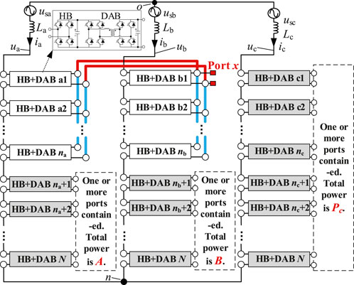
Figure 16. The IDBS-MPET containing D-Port in phase a and phase b.

According to the conclusion drawn in (Shi et al., 2012), in the context of IDBS-MPET employing D-Ports, only symmetric D-Ports are utilized, implying n_a = n_b. Let the power at port Port x be denoted as P_Lx; the total output power of DAB excluding the DAB contained in port Port x in phase a is denoted as A, and similarly, in phase b, it is denoted as B; the total power in phase c is denoted as P_c. By employing the approximation method outlined in Equation 40, the modulation ratios for phases a, b, and c can be derived as follows:

$\left\{\begin{array}{l}{m}_a\approx \frac{\sqrt{3}{U}_p}{N{V}_{dc}}\frac{\left|P_{Lx}+\frac{3A+B-P_c}{2}\right|+\frac{\sqrt{3}}{4}\left|A-B+P_c\right|}{P_{Lx}+A+B+P_c}\\ m_b\approx \frac{\sqrt{3}{U}_p}{N{V}_{dc}}\frac{\left|P_{Lx}+\frac{3B+A-P_c}{2}\right|+\frac{\sqrt{3}}{4}\left|B-A+P_c\right|}{P_{Lx}+A+B+P_c}\\ m_c\approx \frac{\sqrt{3}{U}_p}{N{V}_{dc}}\frac{\sqrt{{\left(A-B\right)}^2+3P_c^2}}{P_{Lx}+A+B+P_c}\end{array}\right.(50)$

Substituting Eq. 50 into Eq. 16, while also considering the proportional relationship between the power of each H-bridge and the phase power as depicted in Figure 18, we can derive the general expression for the modulation ratio of each H-bridge as follows:

(1) For the H-bridges contained within the Port x, the generalized calculation formula for the modulation index of the H-bridge itself is as follows:

$m_{ak}=\frac{\left|P_{Lx}+\frac{3A+B-P_c}{2}\right|+\frac{\sqrt{3}}{4}\left|A-B+P_c\right|}{\frac{n_a}{\sqrt{3}N{m}_N}{P}_{Lx}+\frac{2A{n}_a\left(A+B+P_c\right)}{\sqrt{3}N{m}_N}\frac{1}{P_{Lx}}+\frac{n_a\left(3A+B+P_c\right)}{\sqrt{3}N{m}_N}}(51)$

$m_{bk}=\frac{\left|P_{Lx}+\frac{3B+A-P_c}{2}\right|+\frac{\sqrt{3}}{4}\left|B-A+P_c\right|}{\frac{n_b}{\sqrt{3}N{m}_N}{P}_{Lx}+\frac{2B{n}_b\left(A+B+P_c\right)}{\sqrt{3}N{m}_N}\frac{1}{P_{Lx}}+\frac{n_b\left(A+3B+P_c\right)}{\sqrt{3}N{m}_N}}(52)$

(2) For the H-bridges in phase a and phase b but not contained within the Port x itself, the generalized calculation formula for the modulation index of each H-bridge is as follows:

$m_{aj}=\frac{\left|P_{Lx}+\frac{3A+B-P_c}{2}\right|+\frac{\sqrt{3}}{4}\left|A-B+P_c\right|}{\frac{1}{2\sqrt{3}N{m}_N{P}_{aj}}{P}_{Lx}^2+\frac{3A+B+P_c}{2\sqrt{3}N{m}_N{P}_{aj}}{P}_{Lx}+\frac{A\left(A+B+P_c\right)}{\sqrt{3}N{m}_N{P}_{aj}}}(53)$

$m_{bj}=\frac{\left|P_{Lx}+\frac{3B+A-P_c}{2}\right|+\frac{\sqrt{3}}{4}\left|B-A+P_c\right|}{\frac{1}{2\sqrt{3}N{m}_N{P}_{bj}}{P}_{Lx}^2+\frac{A+3B+P_c}{2\sqrt{3}N{m}_N{P}_{bj}}{P}_{Lx}+\frac{B\left(A+B+P_c\right)}{\sqrt{3}N{m}_N{P}_{bj}}}(54)$

(3) For the H-bridges in phase c, not within the Port x, the generalized calculation formula for the modulation index of each H-bridge is as follows:

$m_{cj}=\frac{\sqrt{{\left(A-B\right)}^2+3P_c^2}}{\frac{P_c}{\sqrt{3}N{m}_N{P}_{cj}}{P}_{Lx}+\left(A+B+P_c\right)\frac{P_c}{\sqrt{3}N{m}_N{P}_{cj}}}(55)$

5.3 The generalized modulation index expression for each H-bridge in the IDBS-MPET containing T-Port

The IDBS-MPET containing the T-Port in phase a, phase b and phase c is illustrated in Figure 17.

Figure 17

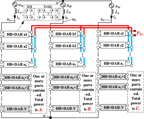
Figure 17. The IDBS-MPET containing T-Port in phase a, phase b and phase c.

Let the power of Port x be P_Lx; the total output power of DAB except for the one contained in Port x in phase a is denoted as A; the total output power of DAB except for the one contained in Port x in phase b is denoted as B; and the total output power of DAB except for the one contained in Port x in phase c is denoted as C. Utilizing the approximation method outlined in Eq. 40, we can determine the modulation ratios for phases a, b, and c as follows:

$\left\{\begin{array}{c}{m}_a\approx \frac{\sqrt{3}{U}_p}{N{V}_{dc}}\frac{\begin{array}{l}\left|\frac{\sqrt{3n_a^2+{\left(n_b-n_c\right)}^2}}{n_a+n_b+n_c}{P}_{Lx}+\frac{3A{n}_a+\left(B-C\right)\left(n_b-n_c\right)}{\sqrt{3n_a^2+{\left(n_b-n_c\right)}^2}}\right|+\\ \frac{\sqrt{3}}{2}\frac{\left|\left(B-C\right)n_a+A\left(n_c-n_b\right)\right|}{\sqrt{3n_a^2+{\left(n_b-n_c\right)}^2}}\end{array}}{P_{Lx}+A+B+C}\\ m_b\approx \frac{\sqrt{3}{U}_p}{N{V}_{dc}}\frac{\begin{array}{l}\left|\frac{\sqrt{3n_b^2+{\left(n_a-n_c\right)}^2}}{n_a+n_b+n_c}{P}_{Lx}+\frac{3B{n}_b+\left(A-C\right)\left(n_a-n_c\right)}{\sqrt{3n_b^2+{\left(n_a-n_c\right)}^2}}\right|+\\ \frac{\sqrt{3}}{2}\frac{\left|\left(C-A\right)n_b+B\left(n_a-n_c\right)\right|}{\sqrt{3n_b^2+{\left(n_a-n_c\right)}^2}}\end{array}}{P_{Lx}+A+B+C}\\ m_c\approx \frac{\sqrt{3}{U}_p}{N{V}_{dc}}\frac{\begin{array}{l}\left|\frac{\sqrt{3n_c^2+{\left(n_a-n_b\right)}^2}}{n_a+n_b+n_c}{P}_{Lx}+\frac{3C{n}_c+\left(A-B\right)\left(n_a-n_b\right)}{\sqrt{3n_c^2+{\left(n_a-n_b\right)}^2}}\right|+\\ \frac{\sqrt{3}}{2}\frac{\left|\left(B-A\right)n_c+C\left(n_a-n_b\right)\right|}{\sqrt{3n_c^2+{\left(n_a-n_b\right)}^2}}\end{array}}{P_{Lx}+A+B+C}\end{array}\right.(56)$

Substituting Eq. 56 into Eq. 16, while also taking into account the proportional relationship between the power of each H-bridge and the phase power as depicted in Figure 17, we can derive the general expression for the modulation ratio of each H-bridge as follows:

(1) The generalized calculation formula for the modulation index of the H-bridges contained within the Port x itself.

$m_{ak}=\frac{\begin{array}{l}\left|\frac{\sqrt{3n_a^2+{\left(n_b-n_c\right)}^2}}{n_a+n_b+n_c}{P}_{Lx}+\frac{3A{n}_a+\left(B-C\right)\left(n_b-n_c\right)}{\sqrt{3n_a^2+{\left(n_b-n_c\right)}^2}}\right|+\\ \frac{\sqrt{3}}{2}\frac{\left|\left(B-C\right)n_a+A\left(n_c-n_b\right)\right|}{\sqrt{3n_a^2+{\left(n_b-n_c\right)}^2}}\end{array}}{\begin{array}{l}\frac{n_a}{\sqrt{3}N{m}_N}{P}_{Lx}+\frac{A\left(A+B+C\right)\left(n_a+n_b+n_c\right)}{\sqrt{3}N{m}_N}\frac{1}{P_{Lx}}+\\ \frac{\left(2A+B+C\right)n_a+A\left(n_b+n_c\right)}{\sqrt{3}N{m}_N}\end{array}}(57)$

$m_{bk}=\frac{\begin{array}{l}\left|\frac{\sqrt{3n_b^2+{\left(n_a-n_c\right)}^2}}{n_a+n_b+n_c}{P}_{Lx}+\frac{3B{n}_b+\left(A-C\right)\left(n_a-n_c\right)}{\sqrt{3n_b^2+{\left(n_a-n_c\right)}^2}}\right|+\\ \frac{\sqrt{3}}{2}\frac{\left|\left(A-C\right)n_b+B\left(n_a-n_c\right)\right|}{\sqrt{3n_b^2+{\left(n_a-n_c\right)}^2}}\end{array}}{\begin{array}{l}\frac{n_b}{\sqrt{3}N{m}_N}{P}_{Lx}+\frac{B\left(A+B+C\right)\left(n_a+n_b+n_c\right)}{\sqrt{3}N{m}_N}\frac{1}{P_{Lx}}+\\ \frac{\left(2B+A+C\right)n_b+B\left(n_a+n_c\right)}{\sqrt{3}N{m}_N}\end{array}}(58)$

$m_{ck}=\frac{\begin{array}{l}\left|\frac{\sqrt{3n_c^2+{\left(n_a-n_b\right)}^2}}{n_a+n_b+n_c}{P}_{Lx}+\frac{3C{n}_c+\left(A-B\right)\left(n_a-n_b\right)}{\sqrt{3n_c^2+{\left(n_a-n_b\right)}^2}}\right|+\\ \frac{\sqrt{3}}{2}\frac{\left|\left(A-B\right)n_c+C\left(n_a-n_b\right)\right|}{\sqrt{3n_c^2+{\left(n_b-n_c\right)}^2}}\end{array}}{\begin{array}{l}\frac{n_c}{\sqrt{3}N{m}_N}{P}_{Lx}+\frac{C\left(A+B+C\right)\left(n_a+n_b+n_c\right)}{\sqrt{3}N{m}_N}\frac{1}{P_{Lx}}+\\ \frac{\left(2C+A+B\right)n_c+C\left(n_a+n_b\right)}{\sqrt{3}N{m}_N}\end{array}}(59)$

(2) For the H-bridges within phase a but not contained within the Port x itself, the generalized calculation formula for the modulation index of each H-bridge is as follows:

$m_{aj}=\frac{\begin{array}{l}\left|\frac{\sqrt{3n_a^2+{\left(n_b-n_c\right)}^2}}{n_a+n_b+n_c}{P}_{Lx}+\frac{3A{n}_a+\left(B-C\right)\left(n_b-n_c\right)}{\sqrt{3n_a^2+{\left(n_b-n_c\right)}^2}}\right|+\\ \frac{\sqrt{3}}{2}\frac{\left|\left(B-C\right)n_a+A\left(n_c-n_b\right)\right|}{\sqrt{3n_a^2+{\left(n_b-n_c\right)}^2}}\end{array}}{\begin{array}{l}\frac{1}{\sqrt{3}N{m}_N{P}_{aj}}\frac{n_a}{n_a+n_b+n_c}{P}_{Lx}^2+\\ \frac{1}{\sqrt{3}N{m}_N{P}_{aj}}\left(A+\frac{n_a}{n_a+n_b+n_c}\left(A+B+C\right)\right)P_{Lx}+\\ \frac{1}{\sqrt{3}N{m}_N{P}_{aj}}A\left(A+B+C\right)\end{array}}(60)$

(3) For the H-bridges within phase b but not contained within the Port x itself, the generalized calculation formula for the modulation index of each H-bridge is as follows:

$m_{bj}=\frac{\begin{array}{l}\left|\frac{\sqrt{3n_b^2+{\left(n_a-n_c\right)}^2}}{n_a+n_b+n_c}{P}_{Lx}+\frac{3B{n}_b+\left(A-C\right)\left(n_a-n_c\right)}{\sqrt{3n_a^2+{\left(n_b-n_c\right)}^2}}\right|+\\ \frac{\sqrt{3}}{2}\frac{\left|\left(A-C\right)n_b+B\left(n_a-n_c\right)\right|}{\sqrt{3n_b^2+{\left(n_a-n_c\right)}^2}}\end{array}}{\begin{array}{l}\frac{1}{\sqrt{3}N{m}_N{P}_{bj}}\frac{n_b}{n_a+n_b+n_c}{P}_{Lx}^2+\\ \frac{1}{\sqrt{3}N{m}_N{P}_{bj}}\left(B+\frac{n_b}{n_a+n_b+n_c}\left(A+B+C\right)\right)P_{Lx}+\\ \frac{1}{\sqrt{3}N{m}_N{P}_{bj}}B\left(A+B+C\right)\end{array}}(61)$

(4) For the H-bridges within phase c but not contained within the Port x itself, the generalized calculation formula for the modulation index of each H-bridge is as follows:

$m_{cj}=\frac{\begin{array}{l}\left|\frac{\sqrt{3n_c^2+{\left(n_a-n_b\right)}^2}}{n_a+n_b+n_c}{P}_{Lx}+\frac{3C{n}_c+\left(A-B\right)\left(n_a-n_b\right)}{\sqrt{3n_c^2+{\left(n_a-n_b\right)}^2}}\right|+\\ \frac{\sqrt{3}}{2}\frac{\left|\left(A-B\right)n_c+C\left(n_a-n_b\right)\right|}{\sqrt{3n_c^2+{\left(n_a-n_b\right)}^2}}\end{array}}{\begin{array}{l}\frac{1}{\sqrt{3}N{m}_N{P}_{cj}}\frac{n_c}{n_a+n_b+n_c}{P}_{Lx}^2+\\ \frac{1}{\sqrt{3}N{m}_N{P}_{cj}}\left(C+\frac{n_c}{n_a+n_b+n_c}\left(A+B+C\right)\right)P_{Lx}+\\ \frac{1}{\sqrt{3}N{m}_N{P}_{cj}}C\left(A+B+C\right)\end{array}}(62)$

6 The general calculation method of power boundary of DC port

The main point for stable operation of IDBS-MPET is to ensure that no H-bridge converter experiences over modulation. As mentioned in Section 4, the key to calculating the power boundary of a port lies in identifying the H-bridge with the maximum risk of over modulation when the port’s transmitted power increases. When the modulation index of this H-bridge reaches 1, the port reaches its power transmission boundary. At this point, using the modulation index general calculation formula derived in Section 5, the power boundary of the port can be calculated.

One of the key features of IDBS-MPET is its ability to effectively connect multiple DC loads and DGs of multiple voltage levels and power levels without the need for additional DC/DC converters. When DC loads and DGs are connected to IDBS-MPET, the power flow directions of the individual DC ports may be different, resulting in inconsistent AC terminal voltage directions of the H-bridge converters within the same phase. If the voltage drop across the inductors L_a, L_b, and L_c is ignored, the three-phase AC output terminal voltage of IDBS-MPET must always match the voltage of the three-phase grid. Therefore, when the AC terminal voltage directions of the H-bridge converters within the same phase are inconsistent, increasing the modulation index of a certain H-bridge may increase the risk of over modulation for the H-bridge with the opposite AC voltage direction. Additionally, considering the injection of zero sequence voltage, the three-phase AC output terminal voltage of IDBS-MPET affects the phase modulation indices of the three phases. Therefore, in the case of inconsistent power flow directions for multiple ports, finding the H-bridge with the maximum risk of over modulation when the power transmission of a certain port increases becomes more complex. This section will propose a method to find the H-bridge with the maximum risk of over modulation.

For IDBS-MPET, when calculating the power boundary of a certain port, it is proposed in this section that the current power of other ports should be taken as known quantities, and each port should be calculated individually to obtain the power boundaries of all ports. This is feasible for the following reasons:

(1) The analytical expressions for the modulation index of H-bridges have been simplified and general calculation formulas have been derived in Section 5, thereby preliminarily reducing the computational workload.

(2) The method to find the H-bridge with the maximum risk of over modulation is proposed in this section. When calculating the power boundary of a certain port, it is not necessary to solve the modulation index for all H-bridges. Only the modulation index of individual H-bridges needs to be calculated, further simplifying the computational workload.

(3) In practical control, the use of DSP controllers allows the calculation time to be controlled at the microsecond level, while the power variation of DGs and DC loads is at the millisecond level. Therefore, calculating the power boundary of each port individually is completely feasible.

The calculation process for the power boundary of DC port, denoted as P_Lx, is as follows:

(1) Identify the H-bridge with the maximum current power in each of the three phases a, b, and c (excluding the H-bridges contained in the port being investigated), denoted as H_a, H_b, H_c, respectively.

(2) Set the modulation index of the port being investigated to 1 and calculate the port’s power limit.

(3) Using the result from step (2), verify whether the modulation indices of the H-bridges H_a, H_b, and H_c are all equal to 1. If all three H-bridges are not over-modulated, then the result from step (2) is the power limit of the port being investigated. Otherwise, proceed to the next step.

(4) Calculate the power of the port being investigated when the modulation indices of the three H-bridges (H_a, H_b, H_c) from step (1) are set to 1, using the derived general analytical expression. Denote these calculated powers as P_Lx,a, P_Lx,b, P_Lx,c, respectively.

(5) The minimum value of the three values obtained in step (4) is the power boundary of the port being investigated, i.e. P_Lx = min{P_Lx,a, P_Lx,b, P_Lx,c}.

7 Simulation verification

In Figure 18, the approximate power boundaries of Port 1 are illustrated using the method proposed in this paper, as Port 2 power varies between 0 and 300 kW within the IDBS-MPET depicted in Figure 7. The load power of Port 3 is set at 200 kW and the load power of Port 4 is set at 400 kW. The circuit parameters of the IDBS-MPET in Figure 7 have been listed in Table 2 in Part A of Section 4. Comparing the approximate calculation with the exact value (obtained through numerical exhaustive search), it can be observed that the accuracy of the approximate method is maintained within a maximum error of 20%, as shown in Figure 19.

Figure 18

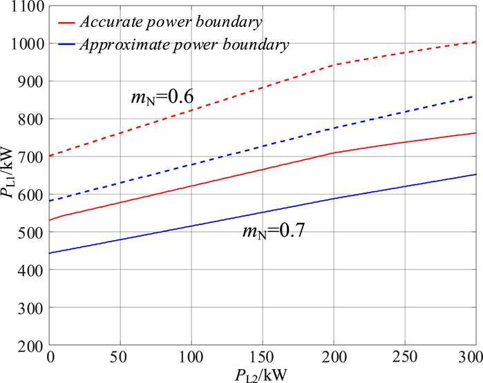
Figure 18. Accurate and approximate power boundary of Port 1 in the IDBS-MPET in Figure 7.

Figure 19

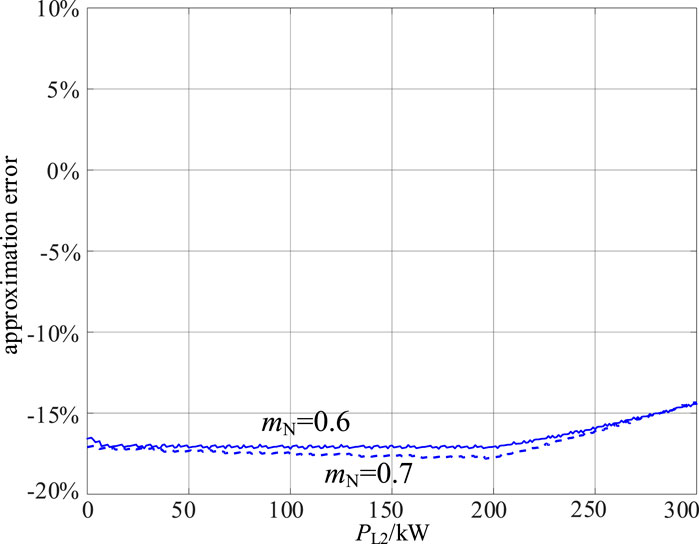
Figure 19. The error between the accurate and approximate power boundary of Port 1 in the IDBS-MPET in Figure 7.

In Figure 20, another structure of the four ports IDBS-MPET is presented. Port 1 and Port 2 are constructed as asymmetrical triple cross-phase-connection type port. Port 3 and Port 4 are constructed as symmetrical double cross-phase-connection type ports. Employing the method proposed in this paper, the approximate power boundaries of Port 3 is derived.

Figure 20

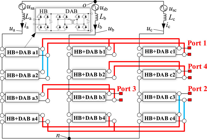
Figure 20. IDBS-MPET with four LVDC ports. Port 1 and Port 2 are constructed as asymmetrical triple cross-phase-connection type port. Port 3 and Port 4 are constructed as symmetrical double cross-phase-connection type ports.

In Figure 21, the approximate power boundaries of Port 3 are illustrated using the method proposed in this paper, as Port 4 power varies between 0 and 250 kW. The load power of Port 1 is set at 400 kW and the load power of Port 2 is set at 400 kW. The circuit parameters of the IDBS-MPET are also the same as them listed in Table 2 in Part A of Section 4. It can be also observed that the accuracy of the approximate method is maintained within a maximum error of 20%, as shown in Figure 22.

Figure 21

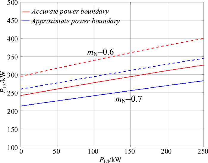
Figure 21. Accurate and approximate power boundary of Port 3 in the IDBS-MPET in Figure 20.

Figure 22

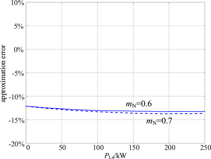
Figure 22. The error between the accurate and approximate power boundary of Port 3 in the IDBS-MPET in Figure 20.

8 Conclusion

This article derives a general calculation method of the DC ports power boundaries of the IDBS-MPET under various power flow directions. Through the analysis of interphase and interbridge power imbalances within IDBS-MPETs, a correlation between H-bridge modulation ratios and DC ports power boundaries was established. Considering the injection of zero sequence voltage, a simplified analytical calculation method for the H-bridge modulation ratio in IDBS-MPETs was derived. A universal calculation method for the H-bridge modulation ratio was established for the IDBS-MPETs containing three basic DC ports (S-Ports, D-Ports, and T-Ports) respectively. Identifying the H-bridge with the highest risk of overmodulation, is crucial for determining the power boundary of a port in IDBS-MPETs. Based on this, a five-step calculation process for IDBS-MPET port power boundaries was proposed. Given that port load changes typically occur on a millisecond scale while the power boundary calculation process is executed on a microsecond scale, sequentially calculating the power boundaries of each port in IDBS-MPETs is feasible. By performing calculations for each port in IDBS-MPETs individually, real-time preventive control of port power can be achieved to avoid exceeding power boundaries. This paper presents power boundary simulation results for two four ports IDBS-MPETs, where the proposed analytical method for power boundary calculation can maintain accuracy within 20%.

Data availability statement

The original contributions presented in the study are included in the article/Supplementary Material, further inquiries can be directed to the corresponding author.

Author contributions

JL: Writing–original draft, Writing–review and editing, Conceptualization, Formal Analysis, Methodology, Validation. JW: Conceptualization, Methodology, Supervision, Writing–review and editing. FX: Writing–review and editing, Methodology, Formal Analysis, Validation, Funding acquisition.

Funding

The author(s) declare that financial support was received for the research, authorship, and/or publication of this article. This work was funded by the National Natural Science Foundation of China (52307193).

Conflict of interest

The authors declare that the research was conducted in the absence of any commercial or financial relationships that could be construed as a potential conflict of interest.

Publisher’s note

All claims expressed in this article are solely those of the authors and do not necessarily represent those of their affiliated organizations, or those of the publisher, the editors and the reviewers. Any product that may be evaluated in this article, or claim that may be made by its manufacturer, is not guaranteed or endorsed by the publisher.

Supplementary material

The Supplementary Material for this article can be found online at: https://www.frontiersin.org/articles/10.3389/fenrg.2024.1422906/full#supplementary-material

References

Abuishmais, I., and Shahroury, F. (2021). “Bidirectional dual active bridge for interfacing battery energy storage systems with DC microgrid,” in Proc. of the International Conference on Electrical, Computer and Energy Technologies (ICECET), Cape Town, South Africa, 09-10 December 2021, 1659–1663. doi:10.1109/icecet52533.2021.9698654

CrossRef Full Text | Google Scholar

Briz, F., Lopez, M., Rodriguez, A., and Arias, M. (2016). Modular power electronic transformers: modular multilevel converter versus cascaded H-bridge solutions. IEEE Ind. Electron. Mag. 10 (4), 6–19. doi:10.1109/mie.2016.2611648

CrossRef Full Text | Google Scholar

Costa, L. F., Carne, G. D., Buticchi, G., and Liserre, M. (2017). The smart transformer: a solid-state transformer tailored to provide ancillary services to the distribution grid. IEEE Power Electron. Mag. 4 (2), 56–67. doi:10.1109/mpel.2017.2692381

CrossRef Full Text | Google Scholar

Huang, A. Q., Crow, M. L., Heydt, G. T., Zheng, J. P., and Dale, S. J. (2011). The future renewable electric energy delivery and management (FREEDM) system: the energy internet. Proc. IEEE 99 (1), 133–148. doi:10.1109/jproc.2010.2081330

CrossRef Full Text | Google Scholar

Huang, A. Q. (2016). Medium-voltage solid-state transformer: technology for a smarter and resilient Grid. IEEE Ind. Electron. Mag. 10 (3), 29–42. doi:10.1109/mie.2016.2589061

CrossRef Full Text | Google Scholar

Huber, E., and Kolar, J. W. (2014). “Volume/weight/cost comparison of a 1MVA 10 kV/400 V solid-state against a conventional low-frequency distribution transformer,” in Proc. IEEE Energy Convers. Congr. Expo, Pittsburgh, PA, USA, 14-18 September 2014, 4545–4552. doi:10.1109/ecce.2014.6954023

CrossRef Full Text | Google Scholar

Huber, J. E., and Kolar, J. W. (2019). Applicability of solid-state transformers in today’s and future distribution grids. IEEE Trans. Smart Grid 10 (1), 317–326. doi:10.1109/tsg.2017.2738610

CrossRef Full Text | Google Scholar

Jia, H., Xiao, Q., and He, J. (2019). An improved grid current and DC capacitor voltage balancing method for three-terminal hybrid AC/DC microgrid. IEEE Trans. Smart Grid 10 (6), 5876–5888. doi:10.1109/tsg.2018.2834340

CrossRef Full Text | Google Scholar

Kolar, J. W., and Ortiz, G. (2014). “Solid-state-transformers: key components of future traction and smart grid systems,” in Proc. Int. Power electron. Conf. Energy convers. Congr. Expo (Hiroshima, Japan: IEEE), 22–35.

Google Scholar

Li, J., Wu, J., and Xiong, F. (2024). Analysis and design of independent DC bus structure multiport power electronic transformer based on maximum power transmission capability of low-voltage DC ports. Energies 17 (5), 1096. doi:10.3390/en17051096

CrossRef Full Text | Google Scholar

Li, K., Wen, W., Zhao, Z., Yuan, L., Cai, W., Mo, X., et al. (2021). Design and implementation of four-port megawatt-level high-frequency-bus based power electronic transformer. IEEE Trans. Power Electron 36 (6), 6429–6442. doi:10.1109/tpel.2020.3036249

CrossRef Full Text | Google Scholar

Liserre, M., Buticchi, G., Andresen, M., De Carne, G., Costa, L. F., and Zou, Z. (2016). The smart transformer: impact on the electric grid and technology challenges. IEEE Ind. Electron. Mag. 10 (2), 46–58. doi:10.1109/mie.2016.2551418

CrossRef Full Text | Google Scholar

Ruiz, F., Perez, M. A., Espinosa, J. R., Gajowik, T., Stynski, S., and Malinowski, M. (2020). Surveying solid-state transformer structures and controls: providing highly efficient and controllable power flow in distribution grids. IEEE Ind. Electron. Mag. 14 (1), 56–70. doi:10.1109/mie.2019.2950436

CrossRef Full Text | Google Scholar

Saleh, S. A. M., Richard, C., St. Onge, X. F., McDonald, K. M., Ozkop, E., Chang, L., et al. (2019). Solid-state transformers for distribution systems–part I: technology and construction. IEEE Trans. Ind. Appl. 55 (5), 4524–4535. doi:10.1109/tia.2019.2923163

CrossRef Full Text | Google Scholar

Shi, J., Zhou, L., and He, X. (2012). Common-duty-ratio control of input-parallel output-parallel (IPOP) connected DC–DC converter modules with automatic sharing of currents. IEEE Trans. Power Electron. 27 (7), 3277–3291. doi:10.1109/tpel.2011.2180541

CrossRef Full Text | Google Scholar

Wang, D., Tian, J., Mao, C., Lu, J., Duan, Y., Qiu, J., et al. (2016). A 10-kV/400-V 500-kVA electronic power transformer. IEEE Trans. Power Electron. 63 (11), 6653–6663. doi:10.1109/tie.2016.2586440

CrossRef Full Text | Google Scholar

Wang, M., Zhang, X., Zhao, T., Ma, M., Hu, Y., Wang, F., et al. (2020). Harmonic compensation strategy for single-phase cascaded H-bridge PV inverter under unbalanced power conditions. IEEE Trans. Ind. Electron. 67 (12), 10474–10484. doi:10.1109/tie.2019.2962461

CrossRef Full Text | Google Scholar

Xue, H., and He, J. (2023). Flexible power control for extending operating range of PV–battery hybrid cascaded H-bridge converters under unbalanced power conditions. IEEE Trans. Industrial Electron. 70 (8), 8118–8128. doi:10.1109/tie.2022.3229317

CrossRef Full Text | Google Scholar

Yan, Y., Bai, H., Foote, A., and Wang, W. (2020). Securing full-power-range zero-voltage switching in both steady-state and transient operations for a dual-active-bridge-based bidirectional electric vehicle charger. IEEE Trans. Power Electron. 35 (7), 7506–7519. doi:10.1109/tpel.2019.2955896

CrossRef Full Text | Google Scholar

Yu, Y., Konstantinou, G., Hredzak, B., and Agelidis, V. G. (2016). Power balance optimization of cascaded H-bridge multilevel converters for large-scale photovoltaic integration. IEEE Trans. Power Electron. 31 (2), 1108–1120. doi:10.1109/tpel.2015.2407884

CrossRef Full Text | Google Scholar

Zhang, Q., and Sun, K. (2019). A flexible power control for PV-battery hybrid system using cascaded H-bridge converters. IEEE J. Emerg. Sel. Top. Power Electron. 7 (4), 2184–2195. doi:10.1109/jestpe.2018.2887002

CrossRef Full Text | Google Scholar

Zhao, B., Song, Q., Li, J., Xu, X., and Liu, W. (2018). Comparative analysis of multilevel-high-frequency-link and multilevel-DC-link DC–DC transformers based on MMC and dual-active bridge for MVDC application. IEEE Trans. Power Electron. 33 (3), 2035–2049. doi:10.1109/tpel.2017.2700378

CrossRef Full Text | Google Scholar

Zhao, B., Song, Q., and Liu, W. (2015). A practical solution of high-frequency-link bidirectional solid-state transformer based on advanced components in hybrid microgrid. IEEE Trans. Power Electron 62 (7), 4587–4597. doi:10.1109/tie.2014.2350459

CrossRef Full Text | Google Scholar

Zhao, T., Wang, G., Bhattacharya, S., and Huang, A. Q. (2013). Voltage and power balance control for a cascaded H-bridge converter-based solid-state transformer. IEEE Trans. Power Electron. 28 (4), 1523–1532. doi:10.1109/tpel.2012.2216549

CrossRef Full Text | Google Scholar