Improved SVM-LSTM-based resource flow forecasting for the low-carbon urban distribution grid

Resource flow supports the delivery of products and services and plays a vital role in the low-carbon urban distribution grid. Therefore, reasonable forecasting of the resource flow is essential for financial decision-making. Through the trained model, the resource flow forecasting process can be simplified and one-click forecasting can be realized. However, this method relies on the selection and optimization of model parameters, where poor parameter choices can significantly impact the forecasting accuracy. This paper first introduces a model for identifying key influencing factors in resource flow data, incorporating an elastic network and gray correlation analysis. Subsequently, a resource flow forecasting method based on improved support vector machines–long- and short term memory (SVM-LSTM) is proposed. Finally, the superior performance of the proposed method is validated through simulations.

1 Introduction

Resource flow is the flow of funds generated by the delivery of products and services in a company’s business process, which plays a crucial role in the low-carbon urban distribution grid (Sanjaya et al., 2019; Zhang and Xia, 2020). Therefore, rational forecasting of the resource flow is essential for financial decision-making, ensuring an optimal cash-holding level that meets the company’s liquidity needs without hindering its growth (Niu and Zhao, 2021; Zhu et al., 2024). For capital-intensive enterprises like power grid companies, with large resource flow scales and complex fund flows, efficient management of resource flow budgeting becomes particularly important (Zhou et al., 2020). One-click resource flow forecasting implies that the power grid resource flow forecasting can be done quickly and accurately through simple operations without complicated and cumbersome steps, which enables companies to respond quickly to market changes, rationalize budget arrangement, and carry out fund management. However, the existing one-click resource flow forecasting methods still face challenges such as the unreasonable identification and selection of factors affecting resource flow prediction and the limitations to a single model. Therefore, achieving effective one-click resource flow forecasting for power grid finances is imperative.

Traditional power grid companies typically employ budgeting methods for resource flow management (Mumtaz et al., 2017; Shen et al., 2023a). Budget compilation is based on various basic data provided by business departments. Each month, budget officers in the business departments aggregate the amount of business documents to be paid the following month and report them to the finance department. The finance department only obtains the total monthly budget amount reported by each business department, and uncertainty exists regarding whether the budget amounts reported by the business departments align with actual economic benefits. To maximize financial benefits and enhance the balance of funds on a monthly and yearly basis, it is crucial to align and integrate business volume and value in the actual planning and budget management process. By establishing a machine learning-based resource flow forecasting model (Zhou et al., 2021; Shen et al., 2023b; Liao et al., 2023), objective data decision-making foundations are provided for budget compilation models. This scientific and comprehensive integration of budget compilation models enhances the auxiliary value in the financial budgeting process, improving overall resource flow budget management capabilities and providing a more comprehensive explanation of the company’s operational status, facilitating high-quality development. Simultaneously, the emphasis on “one-click” underscores the importance of simplifying and integrating the entire resource flow forecasting process compared with “non-one-click.” One-click resource flow forecasting implies completing the forecasting of power grid resource flow through simple operations without the need for complex and cumbersome steps.

The existing machine learning-based resource flow forecasting methods fail to consider the relationship between the accuracy of the forecasting model and the selection of influencing factors. The inclusion of excessive model inputs leads to a dimensionality explosion, thereby affecting the accuracy of resource flow forecasting. Additionally, this method relies on the selection and optimization of model parameters, where poor parameter choices can significantly impact the forecasting accuracy. Simultaneously, relying on a single model for forecasting makes it challenging to capture all relevant factors and variations. Consequently, resource flow forecasting based on a single model may contain errors, ultimately affecting the effectiveness of power grid resource flow forecasts.

To solve the above challenges, first, we propose the elastic network and gray correlation analysis-based influencing factors identifying method. It analyzes the gray correlation of the data and constructs a resource flow data key influencing factor identification model for identification. Second, we propose an improved gray wolf optimizer (IGWO) algorithm based on the elite backward learning strategy with an adaptive convergence factor to expand the search area and increase the diversity of the population. Finally, we construct the improved support vector machine (SVM)–long- and short-term memory (LSTM)-based resource flow forecasting method, which can improve the stability and forecasting accuracy of the model. The main contributions of this paper are summarized herein.

The elastic network and gray correlation analysis-based influencing factor identifying method: An elastic network regression model is constructed to identify the influencing factors closely related to resource flow data. We calculate the gray correlation between each influencing factor and the resource flow data and arrange the factors based on this correlation. It can significantly improve the accuracy of resource flow forecasting.

IGWO based on the elite backward learning strategy with an adaptive convergence factor: For the shortcoming of poor population diversity in the traditional GWO algorithm, we propose the IGWO algorithm to expand the search area. It does not rely on the selection and optimization of model parameters. The IGWO algorithm adopts the elite inverse learning strategy to initialize the population and screen out the elite gray wolves to form a new population. The adaptive degree of convergence factor is adjusted to balance the global search and local optimization ability.

Improved SVM-LSTM-based resource flow forecasting method: We optimize the weights and bias coefficients between the all-connecting layers of the LSTM model and the relevant parameters of the SVM model by using the IGWO algorithm. We construct a combined prediction model consisting of a resource flow prediction model based on IGWO-LSTM and IGWO-SVM to solve the problem that existing resource flow prediction methods based on machine learning rely on a single model for resource flow prediction. We adopt the variance method to determine the weights of the model and then obtain the combined prediction results. It can improve the stability, accuracy, and effectiveness of power grid resource flow forecasting.

2 Related works

In the field of corporate finance, there have been several works that have used resource flow modeling. Specifically, Liu et al. (2023) conducted an empirical study on whether listed small and medium-sized enterprises have financing constraints by constructing a resource flow sensitivity model. Lv (2020) focused on the free resource flow model, which is used for the income assessment of enterprise value and provides a basis for predicting future business development. Han et al. (2020) improved the traditional free resource flow model by using inductive deduction and comparative analysis and established a free resource flow model based on fuzzy bifurcation tree option pricing improvement to better explore the problem of the enterprise value assessment. In conclusion, resource flow is critical for electric utilities because it ensures that the firm has sufficient funds to cover operating expenses, invest in infrastructure, and repay debt. Resource flow forecasting is important to help electric utilities predict and plan for potential cash shortages, make informed financial decisions, and maintain financial stability.

Several time series forecasting models have been widely used for resource flow forecasting. Specifically, Wang (2017) decomposed monthly electricity sales by instantaneous data on electricity sales information and the autoregressive integrated moving average (ARIMA) model to derive an ARIMA model considering seasonal adjustments for forecasting monthly resource flows. Hu et al. (2019) explored the periodicity and non-stationarity characteristics of the data structure by using the segmented multilevel differenced non-stationary time series. The seasonal ARIMA (SARIMA) model was proposed for daily resource flow forecasting. For the difficulty of daily resource flow forecasting due to seasonality and weekend effects, it adjusted and corrected the ARIMA model. In Hans et al. (2019), Weytjens et al. focused on resource flow forecasting techniques. They first discussed classical forecasting techniques such as ARIMA, then multilayer perceptron neural networks, and finally LSTM networks. The evaluation results show that these methods are improved flexibility and accuracy of resource flow forecasting. In Yuan Y. (2018), the calculation of free resource flow in practice was analyzed to predict the free resource flow of enterprises by combining recurrent neural networks with LSTM units. In Yang et al. (2023), the SVM was used for free resource flow forecasting, first analyzing the reasonableness and feasibility for applying SVM to predict the future free resource flow of enterprises, then designing the scheme of SVM to predict the free resource flow according to the relevant theories of SVM, and illustrating the feasibility of SVM to predict the free resource flow in terms of the conclusions of theory and practice. However, previous time series forecasting models have some shortcomings. The output layer of the LSTM is a fully connected layer, which leads to a tendency to fall into local optima when using gradient descent to update coefficients. When a large-scale training sample is input, SVM is difficult to implement and it is not ideal for solving multi-classification problems. At the same time, previous models fail to consider the relationship between the accuracy of the forecasting model and the selection of influencing factors. Therefore, we improve the LSTM and SVM models based on the IGWO algorithm and construct a combined forecasting model to reduce the challenge of capturing relevant factors and changes, as well as improve the stability, accuracy, and effectiveness of power grid resource flow forecasting.

3 Resource flow data key influencing factor identification model

The changes in the power grid resource flow are influenced by a variety of internal and external factors, including the economy, meteorology, and service demand. These influencing factors can be obtained from empirical information or real-time information. However, the source of empirical information is limited and subjective, and it cannot comprehensively and objectively reflect all the influencing factors. Therefore, if the SVM-LSTM model is used directly for power grid resource flow forecasting without fully considering these influencing factors, the accuracy of the resource flow forecasted results will be difficult to ensure. Additionally, the accuracy of the forecasting model is also closely related to the identification and selection of the influencing factors, and the identification and selection of appropriate key influencing factors can further greatly improve the accuracy of resource flow forecasts. However, if too many influential factors are input into the forecasting model, there is a high probability of “dimensional catastrophe,” which will seriously affect the reliability of the forecast. Therefore, choosing the right key influential factors is the basis for accurate forecasting.

The elastic network can suppress overfitting and effectively improve the generalization ability of the resource flow forecasting model through L1 and L2 regularization, and screen out the potential key influencing factors in the case of a large amount of data and many influencing factors. Gray correlation analysis, on the other hand, can effectively assess the correlation between the influencing factors and the target when the amount of data is relatively small and help identify the key influencing factors in the case of incomplete data. Therefore, the combination of elastic network and gray correlation analysis can effectively improve the accuracy and reliability of resource flow influencing factor identification. In this section, an elastic network and gray correlation analysis-based resource flow data key influencing factor identifying method are proposed.

3.1 Elastic network

The elastic network is a regularized linear regression model that combines ridge regression and Lasso regression methods using L1 and L2 norm terms, along with mixed scaling. By adjusting the magnitude of the parameters in the loss function, the elastic network can reduce non-important influencing factors for resource flow forecasting (feature selection) while preserving the complex relationships between important influencing factors in forecasting. It not only satisfies the requirement of stability of the model but also realizes the identification of the characteristic variables. The expression for the loss function of the model is represented as follows Eq. 1:

$J\left(\theta \right)=\frac{1}{2}{\left(X\theta -Y\right)}^T\left(X\theta -Y\right)+\frac{1-r}{2}\alpha \Vert \theta {\Vert }_2^2+r\alpha \Vert \theta {\Vert }_1,(1)$

where r denotes the mixing ratio. In general, the value of the mixing ratio r in the elasticity network ranges from 0 < r < 1. Adjusting the value of the mixing ratio r parameter can adjust the contribution of the two regression methods to the elasticity network. The following special cases can be found in the value of r.

When r = 0, the L1 norm term in the loss function of the elastic network becomes 0, and the elastic network becomes Ridge regression. When r = 1, the L2 norm term of the elastic network loss function becomes 0, and the elastic network becomes Lasso regression. Compared with the ridge and Lasso regression methods alone, the elastic network method can select more feature variables with a higher degree of correlation in the data with higher feature data so as to achieve the purpose of streamlining the model, and at the same time, ensure the stability of the model. Therefore, the elasticity network is more effective in variable selection and model simplification.

3.2 Gray correlation analysis

Gray correlation analysis is an analytical method to measure the degree of correlation between factors based on the similarity of their development trends. By comparing the similarity of data sequences, relative importance of influencing factors in the resource flow can be determined without requiring a large amount of data, which is particularly suitable for analyzing resource flow data in the distribution grid with unclear relationships between variables. The degree of association is used to represent the degree of correlation between two things, which mathematically refers to the degree of similarity between two functions, and the calculation of the gray degree of association is the core of gray correlation analysis. The specific steps for calculating the gray correlation are as follows:

Step 1. Determine the sequence of analysis.

First, let the reference sequence is defined as Eq. 2:

$X_0=\left(x_0\left(1\right),x_0\left(2\right),\dots ,x_0\left(n\right)\right).(2)$

Then, each comparison sequence is defined as Eq. 3:

$\begin{array}{ll}\hfill X_1& =\left(x_1\left(1\right),x_1\left(2\right),\dots ,x_1\left(n\right)\right)\hfill \\ \hfill X_2& =\left(x_2\left(1\right),x_2\left(2\right),\dots ,x_2\left(n\right)\right)\hfill \\ \hfill & \cdots \hfill \\ \hfill X_m& =\left(x_m\left(1\right),x_m\left(2\right),\dots ,x_m\left(n\right)\right).\hfill \end{array}(3)$

Step 2. Remove the dimension of the sequence as Eq. 4:

$\begin{array}{l}{y}_0\left(k\right)=\frac{x_0\left(k\right)}{\frac{1}{n}{\sum }_n^{k=1}{x}_0\left(k\right)},y_i\left(k\right)=\frac{x_i\left(k\right)}{\frac{1}{n}{\sum }_n^{k=1}{x}_i\left(k\right)},\hfill \\ k=\mathrm{1,2},\dots ,n,i=\mathrm{1,2},\dots ,m.\hfill \end{array}(4)$

Step 3. Calculate the correlation coefficients.

The association coefficients of y₀(k) and y_i(k) are as follows Eq. 5:

$\begin{array}{l}{\xi }_i\left(k\right)=\frac{{\mathrm{m}\mathrm{i}\mathrm{n}\mathrm{i}\mathrm{n}\mathrm{i}\mathrm{n}}_i\left|y_0\left(k\right)-y_i\left(k\right)\right|+\rho {\mathrm{m}\mathrm{a}\mathrm{x}\mathrm{m}\mathrm{a}\mathrm{x}}_i\left|y_0\left(k\right)-y_i\left(k\right)\right|}{\left|y_0\left(k\right)-y_i\left(k\right)\right|+\rho {\mathrm{m}\mathrm{a}\mathrm{x}\mathrm{m}\mathrm{a}\mathrm{x}}_i\left|y_0\left(k\right)-y_i\left(k\right)\right|}\hfill \\ \rho \in \left(\mathrm{0,1}\right),k=\mathrm{1,2},\dots ,n,i=\mathrm{1,2},\dots ,m.\hfill \end{array}(5)$

Step 4. Calculate the correlation.

The gray correlation between X_i and X₀ is calculated as follows Eq. 6:

$r_i=\frac{1}{n}{\displaystyle \sum _n^{k=1}}{\xi }_i\left(k\right),k=\mathrm{1,2},\dots ,n,i=\mathrm{1,2},\dots ,m.(6)$

Step 5. Sort by correlation.

The comparative series are sorted according to the gray correlation. The larger the value, the more consistent the trend of the comparative series with the reference series, in other words, the closer the correlation between the two series.

3.3 Elastic network and gray correlation analysis-based influencing factor identifying method

For the enterprise data space of resource flow influencing factors in the spot market of a certain grid, the host is a certain grid enterprise. The dataset is a collection of all controllable data related to a certain grid, including the data generated by the grid’s own service, as well as economic and meteorological influencing factors, and the relationship between these influencing factors and its own data. The host manages the data space through the service, and the high-dimensional data on influencing factors are targeted at the host. For the high-dimensional data on influencing factors, this section proposes an elastic network and gray correlation analysis-based influencing factor identifying method to identify the key influencing factors of the resource flow. The specific process is shown in Figure 1, and the specific steps are as follows:

Figure 1

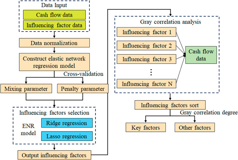
Figure 1. Flowchart of the elastic network and gray correlation analysis-based influencing factor identifying method.

Step 1. The resource flow data and their influencing factor data are normalized.

Step 2. An elastic network regression model is constructed to determine the mixing parameter and the penalty parameter through cross-validation.

Step 3. The obtained parameters are put into the elasticity network regression to calculate the influencing factors and screen out the influencing factors whose regression coefficients are not zero, i.e., the influencing factors that are closely related to the resource flow data.

Step 4. The gray correlation between each influencing factor and the resource flow data is calculated.

Step 5. The influencing factors are sorted according to the gray correlation degree, with as the cut-off point. The factors with a gray correlation greater than are selected as the key factors affecting the resource flow.

4 Improved SVM-LSTM-based resource flow forecasting method

The LSTM neural network is specially designed to solve the problem of long-term dependence (Prakash et al., 2023), which can realize the “memory function” by launching the state of the previous moment into the state of the next moment. LSTM has a gating mechanism that contains the forgetting gate, input gate, and output gate. SVM is a binary classification model, whose basic model is a linear classifier defined as the maximum interval on the feature space (Lin et al., 2018). The core idea of SVM is to transform the input vectors, i.e., the sample pools data into a high-dimensional feature space by some pre-selected non-linear mapping, which transforms the non-linear regression and classification problem into a linear problem to solve, and then constructs an optimal classification hyperplane in this feature space. Resource flow forecasting can be achieved using machine learning algorithms such as LSTM and SVM. However, traditional resource flow forecasting methods rely on the selection and optimization of model parameters, where poor parameter choices can significantly impact the forecasting accuracy. Consequently, resource flow forecasting based on a single model may contain errors, ultimately affecting the effectiveness of power grid resource flow forecasts. As shown in Figure 2, to solve the above problems, we propose an improved SVM-LSTM-based resource flow forecasting method to optimize the LSTM and SVM parameters using IGWO based on an elite backward learning strategy with the adaptive convergence factor and construct the IGWO-LSTM-based resource flow forecasting model and IGWO-SVM-based resource flow forecasting model to improve the accuracy and the effectiveness of power grid resource flow forecasts.

Figure 2

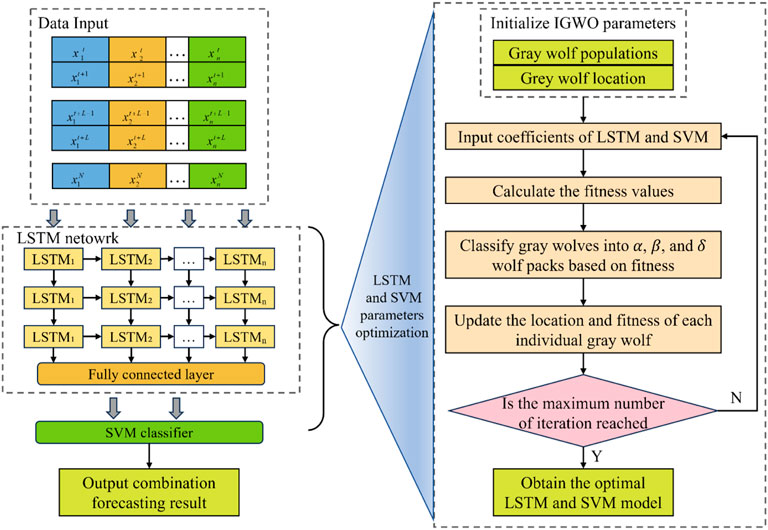
Figure 2. Schematic representation of the improved SVM-LSTM-based resource flow forecasting method.

The improved SVM-LSTM-based resource flow forecasting method process is shown in Figure 3. Specifically, the light green steps represent the input, output, and parameter setting of the algorithm. The steps of skin color represent the common steps of the algorithm. The pink steps indicate the steps that need to be judged in the algorithm. The dark green steps represent the final output. The specific steps are as follows.

Figure 3

Figure 3. Flowchart of the improved LSTM-SVM resource flow forecasting algorithm.

Step 1. The parameters of SVM models and LSTM models are initialized. The number of neurons, learning rate, hidden layer nodes, training times, and other LSTM parameters are initialized. Environmental factors and historical resource flows are set as the initial input features of the LSTM model and resource flows as output features. Set the maximum number of iterations and the range of the SVM penalty factor and the kernel function parameter. The LSTM neural network and SVM model are two common traditional prediction algorithms.

Step 2. Initial training of SVM models and LSTM models. The LSTM model is used for initial training, and after reaching the number of training times, the parameters between the connected layers will be exactly the same. At the same time, based on the initial setup range parameters, the training set is trained by the SVM.

Step 3. IGWO parameters, gray wolf populations, and the randomly generated initial gray wolf population are initialized. The GWO algorithm is an optimized searching method inspired by the prey hunting activities of gray wolves (Liao et al., 2022). However, the initial population generation method of GWO is random initialization, which is prone to the problem that gray wolves are too dispersed or gathered in the same area, which leads to the shortcoming of poor population diversity in traditional GWO, and has a greater negative impact on the later iterative optimization. Therefore, in this paper, we choose to use the elite reverse learning strategy to initialize the population, which can expand the search area of the algorithm and increase the diversity of the population.

The elite reverse learning strategy is to find the inverse solution to a feasible solution of a problem, expanding the search region. Set x(t) to be a solution of the t th iteration with the inverse solution x′(t), which is given as Eq. 7

$x_j^{\prime }\left(t\right)=k\left(a_j\left(t\right)+b_j\left(t\right)\right)-x_j\left(t\right).(7)$

The accuracy, convergence, and results of GWO are closely tied to how well the initial gray wolf population. The accuracy and results of GWO are closely related to the goodness of the initial gray wolf population. To summarize, in this paper, we randomly generate an initial population and then select ξ elite gray wolves with the highest fitness through inverse learning to form a new gray wolf population.

In the traditional gray wolf algorithm, $\vec{a}$ is a convergence factor that decreases linearly from 2 to 0 with the number of iterations. In this paper, during the iteration process of the algorithm, the adaptive degree of convergence factor $\vec{a}$ is adjusted in order to balance the global search and local optimization ability of the GWO after the creation of a new population by using the inverse learning strategy, and the improved formula is as follows Eq. 8:

$a\left(t\right)=\frac{1-{\left(t/T\right)}^2}{1-\mu {\left(t/T\right)}^2},(8)$

where T is the total number of iterations. μ is the interval [0,3] of non-linear modulation of the index.

Step 4. Initial training of SVM models and LSTM models. The LSTM model is trained initially. After reaching the training count, the parameters between the connection layers of the LSTM model will be exactly the same. At the same time, based on the initial setup range parameters, the training set is trained by the SVM to get the accuracy as the fitness of the gray wolf.

Step 5. IGWO is utilized to optimize the LSTM model. Since the output layer of the LSTM is a fully connected layer, the coefficients of the LSTM are commonly updated by the gradient descent method, which is prone to fall into the local optimal solution. So after the initial training of the LSTM model, the weights and bias coefficients between the fully connected layers of the LSTM model are optimized by using the IGWO to improve the forecasting accuracy of the model.

Step 6. The fully connected layer parameters of the optimal LSTM model are obtained.

Step 7. The IGWO optimized parameters are replaced with the LSTM model fully connected layer parameters. Step 8. IGWO is utilized to optimize the SVM model.

The fitness values of individual gray wolves are calculated, gray wolves are classified into α, β, and δ wolf packs based on the best fitness value, and the location and fitness of each individual gray wolf are updated. If the maximum number of iterations is reached, the optimization search ends and outputs the optimal parameters c and g, and the optimal SVM model is obtained. Otherwise, step 8 is repeated to continue searching for parameters.

Step 9. Constructing the combined forecasting model.

Constructing a combined forecasting model can combine the advantages of each individual model to improve the stability and forecasting accuracy of the model. In this paper, the variance method is used to determine the weights of the model, which are calculated as follows.

The variance corresponding to each forecasting model is calculated as Eq. 9:

$D=\frac{1}{n}\left[{\left(e_1-\bar{e}\right)}^2+{\left(e_2-\bar{e}\right)}^2+\cdots +{\left(e_n-\bar{e}\right)}^2\right],i=\mathrm{1,2},(9)$

where n denotes the number of test samples; e₁, e₂, …, e_n denote the percentage error of each test sample; and $\bar{e}$ denotes the average percentage error of the n test sample.

The weights of the individual models are calculated from the variances as Eqs 10, 11:

${\omega }_1=1/\left[D_1\left(1/D_1+1/D_2\right)\right],(10)$

${\omega }_2=1/\left[D_2\left(1/D_1+1/D_2\right)\right].(11)$

The weights are multiplied with the corresponding forecast results, and then, the forecast results after multiplying by the weights are added together to obtain the combined forecast results which is given by Eq. 12.

$F={\omega }_1{F}_1+{\omega }_2{F}_2,(12)$

where F denotes the forecasting result. F₁ and F₂ denote the individual forecasting results of the IGWO-LSTM model and the IGWO-SVM model, respectively.

5 Simulation results

To validate the impact on resource flow forecasting after using the resource flow data key influencing factor identification model, this paper adopted the relevant data on a province for each month from 2016 to 2019. Through the proposed mining method of influencing factors based on elastic network and gray correlation analysis, the four factors with the highest gray correlation, which have the greatest influence on the resource flow data, are finally screened out as the input data for resource flow forecasting. The top eight gray correlations between each factor and resource flow data are shown in Table 1. It can be seen that the gray correlation of temperature is high. The reason is that temperature will significantly affect the power consumption of power users. Using electrical appliances for cooling or heating will generate a lot of electricity consumption, which will affect the resource flow in the power grid.

Table 1

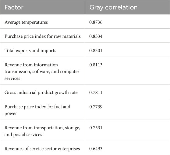
Table 1. Gray correlations of factors with resource flow data.

On this basis, the daily resource flow data on the provincial power grid from 1 January 2022 to 31 December 2022 are forecasted. In order to verify the effectiveness of the improved SVM-LSTM-based resource flow forecasting method proposed in this paper which optimizes SVM and LSTM based on IGWO, the GWO-SVM forecasting model (Jiang et al., 2020) and the LSTM method (Rana and Kim, 2019) are used to compare with the model proposed in this paper. The simulation parameters are shown in Table 2 (Duan et al., 2023).

Table 2

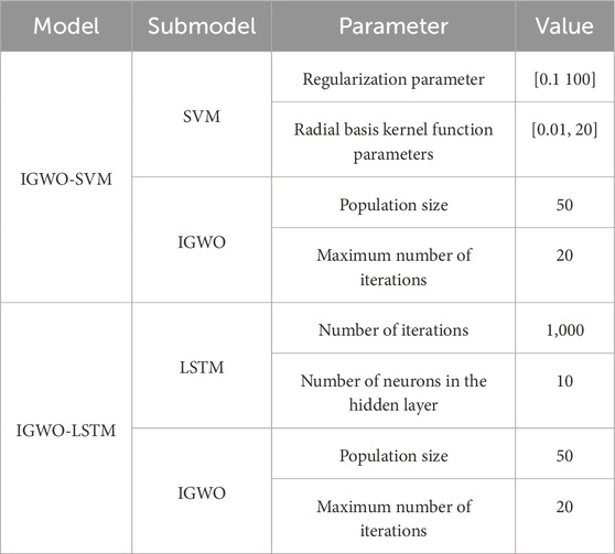
Table 2. Simulation parameters.

Table 3 illustrates the comparison of forecasting values of resource flow obtained by different algorithms with actual values. The simulation results demonstrate that the forecasting values of the resource flow obtained by the proposed algorithm are closer to actual values than those obtained by GWO-SVM and LSTM. The reason is that the proposed algorithm combines the advantages of the LSTM model and the SVM model, and optimizes the parameters of the LSTM model and the SVM model using the IGWO algorithm.

Table 3

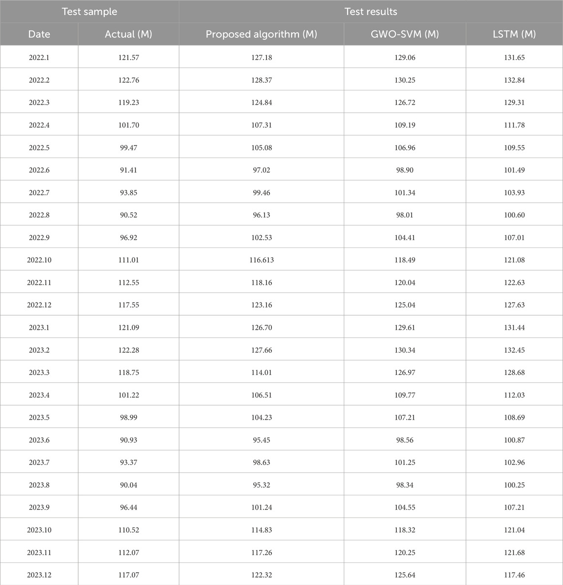
Table 3. Simulation parameters.

Figure 4 illustrates the number of iterations at convergence and the average error of the proposed method versus influencing factors. The horizontal coordinate indicates the number of influencing factors. The number of iterations at convergence is minimized, and the average error is minimized when considering the four factors. The proposed elastic network method combines the ridge regression and Lasso regression methods and uses the L1 and L2 norm terms in combination with the mixing ratio (mix ratio), which not only meets the model’s need for stability but also realizes the identification of the feature variables.

In order to evaluate the predictive performance of the improved SVM-LSTM model more accurately, this paper adopts the following four indicators including the mean absolute percentage error (MAPE), root mean square error (RMSE), mean absolute error (MAE), and coefficient of determination. The prediction error analysis is conducted to reflect the prediction accuracy of the model. The indicators are calculated as follows Eqs 13–16:

$MAPE=\frac{1}{N}{\displaystyle \sum _{n=1}^N}\left|\frac{{\widehat{y}}_n-y_n}{y_n}\right|,(13)$

$RMSE=\sqrt{\frac{1}{N}{\displaystyle \sum _{n=1}^N}{\left({\widehat{y}}_n-y_n\right)}^2},(14)$

$MAE=\frac{1}{N}{\displaystyle \sum _{n=1}^N}\left|{\widehat{y}}_n-y_n\right|,(15)$

$R^2=1-\frac{{\sum }_{n=1}^N\left|y_n-{\tilde{y}}_n\right|}{{\sum }_{n=1}^N\left|y_n-\bar{y}\right|},(16)$

Figure 4

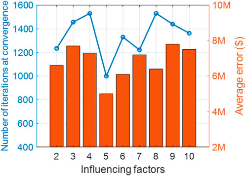
Figure 4. Number of iterations at convergence and average error versus influencing factors.

where ${\widehat{y}}_n$ is the forecasted value. y_n is the actual value. $\bar{y}$ is the average value of the actual values. ${\tilde{y}}_n$ is the simulated value of the variable for the statistical model. N is the forecasted sample size.

Figures 5–7 illustrate the comparison of forecasted and actual resource flow values versus different algorithms, where Figure 5 shows the scatterplot of actual and forecasted values of the proposed model, Figure 6 shows the scatterplot of actual and forecasted values of the GWO-SVM model, and Figure 7 shows the scatterplot of actual and forecasted values of the LSTM model. The simulation results demonstrate that the coefficient of determination of the proposed algorithm is 11.39% and 22.22% higher than those of GWO-SVM and LSTM, respectively. The reason is that the proposed algorithm fuses the IGWO-LSTM model and the IGWO-SVM model to synthesize the advantages of the two forecasting models and obtain a more accurate forecasting result.

Figure 5

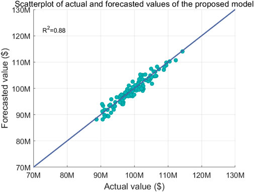
Figure 5. Scatterplot of actual and forecasted values of the proposed model.

Figure 6

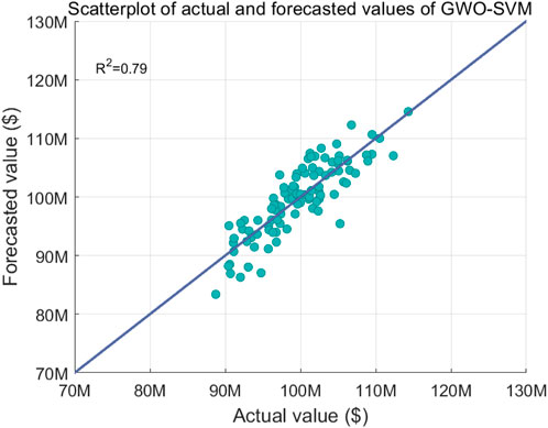
Figure 6. Scatterplot of actual and forecasted values of GWO-SVM.

Figure 7

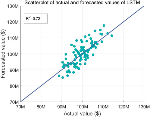
Figure 7. Scatterplot of actual and forecasted values of LSTM.

Figure 8 illustrates the MAPE versus iterations. MAPE is used to measure the accuracy of the data dimensionality reduction model. Compared to GWO-SVM and LSTM, the MAPE of the proposed algorithm is reduced by 44.51% and 31.65%, respectively. This algorithm optimizes the weights and bias coefficients between the fully connected layers of the LSTM model through IGWO to improve the forecasting accuracy of the model.

Figure 8

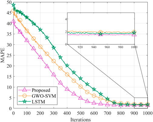
Figure 8. MAPE versus iterations.

Table 4 illustrates the MAE, RMSE, and MAPE versus different algorithms. MAPE is used to measure the accuracy of the data dimensionality reduction model. For these three metrics, the evaluation results of the proposed model in this section are optimal, which are 6.4309, 7.7090%, and 1.52%, respectively. Therefore, from analyzing the overall evaluation metrics of the models, it can be found that the overall stability of the proposed model in this section is the best, followed by the LSTM model, and the GWO-SVM model is the worst.

Table 4

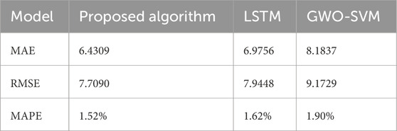
Table 4. Simulation parameters.

6 Conclusion

In this paper, we have introduced an improved SVM-LSTM-based efficient resource flow forecasting for power grid enterprise. First, we presented a resource flow data key influencing factor identification model, which can greatly improve the accuracy of resource flow forecasts by selecting appropriate influencing factors. Subsequently, we proposed an improved SVM-LSTM-based resource flow forecasting method to improve the accuracy and the effectiveness of power grid resource flow forecasts. Finally, we validated the superior performance of the proposed method through simulations. The simulation results prove the usability and effectiveness of the proposed forecasting model. Furthermore, the coefficient of determination of the proposed algorithm is 11.39% and 22.22% higher than those of GWO-SVM and LSTM, respectively. Compared to GWO-SVM and LSTM, the MAPE of the proposed algorithm is reduced by 44.51% and 31.65%, respectively. Moving forward, we aim to investigate methods to ensure the traceability of financial data.

Data availability statement

The original contributions presented in the study are included in the article/Supplementary Material; further inquiries can be directed to the corresponding author.

Author contributions

LS: conceptualization, formal analysis, investigation, methodology, software, validation, writing–original draft, and writing–review and editing.

Funding

The author(s) declare that financial support was received for the research, authorship, and/or publication of this article. This research was supported by the development and implementation project of State Grid Jibei Electric Power Company Limited (grant number 71018E22002U).

Conflict of interest

Author LS was employed by State Grid Jibei Electric Power Company Limited.

The authors declare that this study received funding from the development and implementation project of State Grid Jibei Electric Power Company Limited. The funder had the following involvement in the study: the study design, collection, analysis, interpretation of data, the writing of this article, and the decision to submit it for publication.

Publisher’s note

All claims expressed in this article are solely those of the authors and do not necessarily represent those of their affiliated organizations, or those of the publisher, the editors, and the reviewers. Any product that may be evaluated in this article, or claim that may be made by its manufacturer, is not guaranteed or endorsed by the publisher.

References

Duan, Z.-m., Ji, W., Xue, Y., and Xi, Z. (2023). Spatio-temporal analysis of water quality based on gray wolf optimization and support vector machines (GWO-SVM): a case study from dongting lake, China, 626–629.

Google Scholar

Han, X., Fu, J., and Zhao, C. (2020). Improved free cash flow evaluation model based on fuzzy binary tree. J. Liaoning Tech. Univ. Sci. (03), 161–167.

Google Scholar

Hans, W., Enrico, L., and Enrico, L. (2019). Cash flow prediction:MLP and LSTM compared to ARIMA and prophet. Electron. Commer. Res. 21 (prepublish), 1–21. doi:10.1007/s10660-019-09362-7

CrossRef Full Text | Google Scholar

Hu, R., Jin, X., Wang, D., Wang, M., and Xiaoran, W. (2019). Prediction for the daily cash flow based on nonstationary time series, Applied Mathematics-A Journal of Chinese Universities. Ser. A 34 (03), 253–263. doi:10.13299/j.cnki.amjcu.002078

CrossRef Full Text | Google Scholar

Jiang, T., Wang, Y., and Li, Z. (2020). Fault diagnosis of three-phase inverter based on CEEMDAN and GWO-SVM, 2362–2368.

Google Scholar

Liao, H., Zhou, Z., Liu, N., Zhang, Y., Xu, G., Wang, Z., et al. (2023). Cloud-edge-device collaborative reliable and communication-efficient digital twin for low-carbon electrical equipment management. IEEE Trans. Industrial Inf. 19 (2), 1715–1724. doi:10.1109/tii.2022.3194840

CrossRef Full Text | Google Scholar

Liao, W., Zhou, L., Zhang, C., Wang, D., Zhang, J., and Guo, L. (2022). A method for discriminating the moisture status of OIP bushing based on dissado-hill and GWO-HMM model. IEEE Trans. Industry Appl. 58 (2), 1512–1520. doi:10.1109/tia.2021.3137368

CrossRef Full Text | Google Scholar

Lin, Z., Xiong, Y., Cai, G., Dai, H., Xia, X., Tan, Y., et al. (2018). Quantification of parkinsonian bradykinesia based on axis-angle representation and SVM multiclass classification method. IEEE Access 6, 26895–26903. doi:10.1109/access.2018.2835463

CrossRef Full Text | Google Scholar

Liu, Y., Wang, H., and Zheng, Q. (2023). Research on the influence of supply chain finance on the financing of smaland medium-sized enterprises under cash flow sensitivity model. Financial theory Teach. (03), 45–49. doi:10.13298/j.cnki.ftat.2023.03.004

CrossRef Full Text | Google Scholar

Lv, Y. (2020). Discussion on working capital–using free cash flow model to calculate enterprise value. Apprais. J. China (03), 58–64.

Google Scholar

Mumtaz, S., Alsohaily, A., Pang, Z., Rayes, A., Tsang, K. F., and Rodriguez, J. (2017). Massive internet of things for industrial applications: addressing wireless IIoT connectivity challenges and ecosystem fragmentation. IEEE Ind. Electron. Mag. 11 (1), 28–33. doi:10.1109/mie.2016.2618724

CrossRef Full Text | Google Scholar

Niu, T., and Zhao, X. (2021). Impacts of managerial overconfidence and agency costs on cash holdings within blockchain firms. IEEE Access 9 (99), 141453–141466. doi:10.1109/access.2021.3119613

CrossRef Full Text | Google Scholar

Prakash, S., Jalal, A. S., and Pathak, P. (2023). Forecasting COVID-19 pandemic using prophet, LSTM, hybrid GRU-LSTM, CNN-LSTM, Bi-LSTM and Stacked-LSTM for India, 1–6.

Google Scholar

Rana, A., and Kim, K. K. (2019). ECG heartbeat classification using a single layer LSTM model, 267–268.

Google Scholar

Sanjaya, N., Ajay, K. J., and Anirudh, P. S. (2019). Financial analysis of 18kW solar photovoltaic baidi microgrid at baidi, tanahun, Nepal. J. Inst. Eng. 15 (1), 229–236. doi:10.3126/jie.v15i1.27739

CrossRef Full Text | Google Scholar

Shen, Z., Ding, F., Jolfaei, A., Yadav, K., Vashisht, S., and Yu, K. (2023b). Deformablegan: generating medical images with improved integrity for healthcare cyber physical systems. IEEE Trans. Netw. Sci. Eng. 10 (5), 2584–2596. doi:10.1109/tnse.2022.3190765

CrossRef Full Text | Google Scholar

Shen, Z., Ding, F., Yao, Y., Bhardwaj, A., Guo, Z., and Yu, K. (2023a). A privacy-preserving social computing framework for health management using federated learning. IEEE Trans. Comput. Soc. Syst. 10 (4), 1666–1678. doi:10.1109/tcss.2022.3222682

CrossRef Full Text | Google Scholar

Wang, C. (2017). Study on monthly electricity sales forecast based on season adjusted ARIMA model. Tianjin, China: Tianjin University.

Google Scholar

Yang, X., Liao, Z., Liu, L., and Wang, C. (2023). Power data sharing scheme based on blockchain and attribute-based encryption. Power Syst. Prot. Control 51 (13), 169–176. doi:10.19783/j.cnki.pspc.221491

CrossRef Full Text | Google Scholar

Zhang, J., and Xia, C. (2020). Structured multi-agent-based model for bankruptcy contagion with cash flow. IEEE Access 8 (99), 171716–171729. doi:10.1109/access.2020.3024711

CrossRef Full Text | Google Scholar

Zhou, Z., Wang, B., Dong, M., and Ota, K. (2020). Secure and efficient vehicle-to-grid energy trading in cyber physical systems: integration of blockchain and edge computing. IEEE Trans. Syst. Man, Cybern. Syst. 50 (1), 43–57. doi:10.1109/tsmc.2019.2896323

CrossRef Full Text | Google Scholar

Zhou, Z., Wang, Z., Yu, H., Liao, H., Mumtaz, S., Oliveira, L., et al. (2021). Learning-based URLLC-aware task offloading for internet of health things. IEEE J. Sel. Areas Commun. 39 (2), 396–410. doi:10.1109/jsac.2020.3020680

CrossRef Full Text | Google Scholar

Zhu, X., Ma, F., Ding, F., Guo, Z., Yang, J., and Yu, K. (2024). A low-latency edge computation offloading scheme for trust evaluation in finance-level artificial intelligence of things. IEEE Internet Things J. 11 (1), 114–124. doi:10.1109/jiot.2023.3297834

CrossRef Full Text | Google Scholar