A new dynamic state estimation method for distribution networks based on modified SVSF considering photovoltaic power prediction

The fluctuations brought by the renewable energy access to the distribution network make it difficult to accurately describe the state space model of the distribution network’s dynamic process, which is the basis of the existing dynamic state estimation methods such as the Kalman filter. The inaccurate state space model directly causes an error of dynamic state estimation results. This paper proposed a new dynamic state estimation method which can mitigates the impact of renewable energy fluctuation by considering PV power prediction in establishing distribution network state space model. Firstly, the proposed method mitigates the impact of renewable energy fluctuation by considering PV power prediction in establishing distribution network state space model. Secondly, SVSF filter is introduced to achieve more accurate estimation under noise. The case study and evaluations are carried out based on MATLAB simulation. The results prove that the smooth variable structure filter with photovoltaic power prediction has a better dynamic state estimation effect under the fluctuation of the distribution network compared with the existing Kalman filter.

1 Introduction

As a renewable energy source, photovoltaic (PV) technology offers great potential. It is convenient to install, less subject to geographical restrictions, and can be easily arranged (Khalid et al., 2023). PV is an important part of clean energy that promotes sustainable energy development and protects the environment, which is an important reason for its widespread acceptance in power systems. However, the large-scale integration of photovoltaic systems into the distribution network presents significant difficulties. The fluctuation of several PV accesses to distribution networks causes significant difficulties in stability and controllability. To control the risks of distribution networks, dynamic state estimation is one of the necessary methods. Dynamic state estimation models and measurement data are used to perform a calculation based on a state-space model (Lupeng et al., 2023) or other prediction methods to obtain state estimation and prediction values, achieving the purpose of dynamic tracking and prediction of the system.

Existing dynamic state estimation methods usually use the Kalman filter to estimate the dynamic system’s linear state. Its greatest advantage is that it can be calculated in different situations without modification. To solve the problem of nonlinear system prediction, the extended Kalman filter was proposed, which can track the nonlinear dynamic system state by obtaining the Jacobian matrix of the transition matrix and ignoring the high-order components in the Taylor expansion (Mandal et al., 1995). However, calculating the Jacobian matrix in every calculation will result in slow convergence speed, and ignoring high-order components reduces the accuracy of the dynamic state results. Therefore, the unscented Kalman filter (UKF) (Wang et al., 2012) was proposed to further overcome these limitations by using unscented transformation to map the statistical distribution of the state space to the measurement space through the measurement equation and using the propagation of sampling points instead of nonlinear function transformation so that the high-order terms in the nonlinear measurement equation do not need to be discarded during the process, avoiding linearization errors. However, the unscented transformation will cause the mapping of the state space to fall outside the feasible domain of the measurement space, making the sampling points meaningless. Therefore, Sharma et al. (2017) introduced the cubature Kalman filter (Haykin and Arasaratnam, 2009) into dynamic state estimation. The cubature Kalman filter is based on the third-order spherical radial volumetric criterion and uses a set of volumetric points instead of UKF sampling points. The sampling rules and weighting strategies are determined, ensuring strong applicability while maintaining high accuracy and stability even when dealing with problems involving many state variables.

As distributed power generation gradually occupies a higher proportion in the distribution networks, traditional distribution networks are shifting toward active distribution networks (ADNs), and a large number of renewable energy generation devices, such as photovoltaics, are connected to active distribution networks, highlighting the nonlinear issues. The state-space model of the power system changes frequently, and traditional dynamic state estimation can no longer meet the accurate requirements because existing Kalman filters based on the state-space model make it difficult to accurately describe the distribution networks and reflect the actual operation of the distribution network. Moreover, due to the random fluctuation of renewable energy, the state of the distribution network changes frequently and can become unstable. So, the dynamic state estimation method based on Kalman filters, which is suitable for traditional stable distribution networks, is not suitable for active distribution networks.

Recent studies, such as Guanghua et al. (2022), have tried to address these problems of existing Kalman filters. Furthermore, the smoothing variable structure filter (SVSF) has emerged as an efficient solution. This filter is a “predictive–corrective” estimator with good stability and robustness for modeling uncertainties and disturbance noise with given upper limits. Habibi and Burton (2003) proposed a filtering algorithm based on an uncertain model, which introduced a smooth boundary layer and a sliding membrane into the calculation of filtering gain, and proposed the first smooth variable structure filter. Due to the existence of uncertain random interference in practical systems, Habibi (2007) obtained an approximate optimal smooth boundary layer by taking the partial derivative of the estimation error covariances. Gadsden and Habibi (2013) extended the boundary layer to a full matrix form and obtained a smooth variable structure filter with an optimal smooth boundary layer Jiawei et al. (2023) used UKF to predict the real-time operating levels of the state variables and model PV power intervention by predicting the photovoltaic power. The limitations of the previous works in dynamic state estimation are shown in Table 1.

Table 1

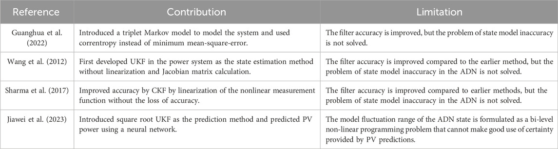
Table 1. Limitations of previous works in dynamic state estimation.

To alleviate the influence of photovoltaic fluctuations on the relatively stable original state-space model of the distribution network, which causes inaccuracies in the existing dynamic state estimation methods such as the Kalman filter, this paper introduces the SVSF as the prediction model in the dynamic state estimation of distribution networks and integrates photovoltaic prediction methods mainly based on the BP-neural network. The photovoltaic power prediction is innovatively used to model the fluctuation influence of the photovoltaic power at the next moment on the voltage vector, which effectively improves the accuracy of estimation in active distribution networks.

This paper proposes a new dynamic state estimation method for distribution networks-based modified SVSF under photovoltaic access. The main contributions of the paper are as follows:

(1) By predicting the photovoltaic power based on real-time weather data when modeling the distribution network state-space model, photovoltaics are integrated into the dynamic state estimation system in SVSF. This enables modeling the impact of PV on the state of the distribution network at the next moment. In addition, the effect of PV power fluctuation on the dynamic state estimation accuracy of the distribution network is effectively reduced.

(2) By introducing the SVSF, a dynamic state estimation method for distribution networks with photovoltaic power prediction is proposed. The proposed method alleviates the problem caused by the frequent changes in the state-space model due to the photovoltaic power fluctuations. It can improve the robustness under data noise and the accuracy of the dynamic state estimation.

2 Photovoltaic power prediction using the BP-neural network

This section considers photovoltaic power generation equipment as the objective to introduce the combination of new energy power generation equipment represented by photovoltaics and the dynamic state estimation algorithm. Photovoltaic power prediction needs to start with the correlation between photovoltaic power and the related meteorological factors. The proposed method selected appropriate and closely related meteorological factors for prediction training and avoided invalid training interference with prediction results. The Pearson correlation coefficient analysis method is selected to standardize the correlation between the meteorological factors and photovoltaic power generation capacity.

Most studies in Table 2 believe that the power of photovoltaic power generation equipment has a strong correlation with solar radiation, ambient temperature, and relative humidity. At the same time, different correlation coefficients may be caused by different photovoltaic power generation equipment used in different studies, different weather and meteorological conditions (Hammad et al., 2021), and other reasons (Aljdaeh et al., 2021). However, most studies believe that solar radiation is the preferred factor affecting photovoltaic power generation equipment.

Table 2

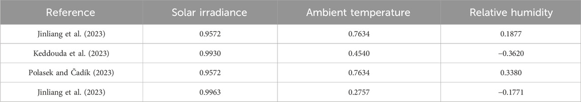
Table 2. Pearson correlation coefficient of different factors.

When training the prediction network that meets the local geographical conditions and the installed equipment, it is necessary to conduct correlation analysis on the medium- and long-term real machine data and the meteorological data of similar conditions of the equipment that has been installed locally. Based on this correlation analysis, the prediction model is designed and trained.

A relatively simple BP-neural network is selected as the prediction network for photovoltaic power prediction. The topology structure of the BP-neural network is shown in Figure 1.

Figure 1

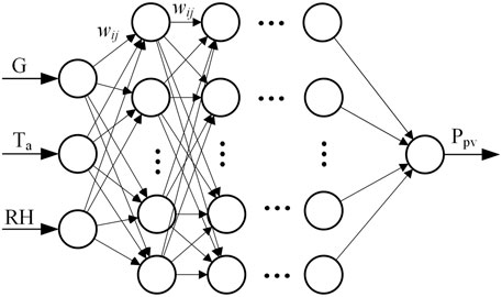
Figure 1. Topology structure of the BP-neural network.

The core of the BP-neural network is the forward and backward propagation process of the neurons in the hidden layer (Zhao, 2015). Eq. 1 represents forward propagation, where $w_{ij}$ is the weight between neuron $i$ in the previous layer and neuron $j$ in this layer. The threshold of neuron $j$ in this layer is $b_j$, and the output of the neuron in this layer is $x_j$. $f$ is the activation function, which is generally chosen as the sigmoid function.

$\begin{array}{c}{\mathbf{S}}_{\mathbf{i}}={\displaystyle {\sum }_{\mathbf{i}=\mathbf{0}}^{\mathbf{m}-\mathbf{1}}}{\mathbf{w}}_{\text{ij}}{\mathbf{x}}_{\mathbf{i}}+{\mathbf{b}}_{\mathbf{j}}\\ {\mathbf{x}}_{\mathbf{j}}=\mathbf{f}\left({\mathbf{S}}_{\mathbf{j}}\right)\end{array}.(1)$

In other words, the output value of each neuron is adjusted under the intervention of the activation function based on the output values of all the nodes in the previous layer and the current neuron value. During training, after the new output is formed by forward propagation, according to the error between the output and actual values, the Widrow–Hoff learning rule reverses the error along the path of forward propagation and modifies the weights of each neuron in each hidden layer, and it continuously repeats this learning process to make the error between the output and actual values as small as possible.

The input variables of photovoltaic prediction are based on short-term weather forecast factors $\left\{G,\right.T_a\left.,RH\right\}$, namely, solar radiation $G\left(W\cdot m^2\right)$, ambient temperature $T_a$($C°$), and air humidity $RH$ ($\%$). The output variable is photovoltaic power $\left\{P_{pv}\right\}$, and its prediction effect is shown in Figure 2: the mean absolute percentage error (MAPE) is 16.412%, and the root-mean-square error (RMSE) is 1.3736.

Figure 2

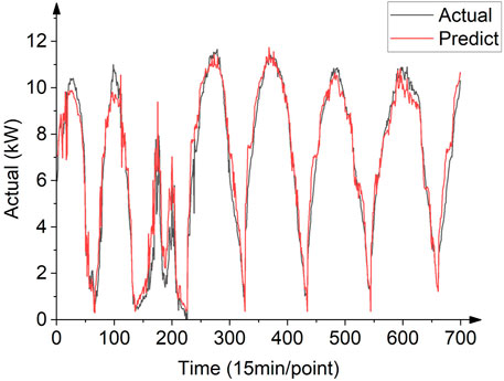
Figure 2. Results of solar power prediction.

3 Improved dynamic state estimation method with the smooth variable structure filter

The smooth variable structure filter is a “predictive–corrective” estimator that can effectively estimate the state of a system. The structure of SVSF is shown in Figure 3. Assuming a certain state variable is x, its estimated value is $\widehat{x}$. The initial value of $\widehat{x}$ is selected based on probability distribution or prior knowledge. By utilizing noise and error information and using SVSF gain to switch on both sides of the existence subspace, $\widehat{x}$ is forced to exist around the subspace. When $\widehat{x}$ is outside the subspace, a discontinuous gain is used to ensure stable calculation of the algorithm. When $\widehat{x}$ enters the subspace, a continuous gain is used for dynamic state estimation, thereby eliminating certain error effects. For SVSF, the premise of effectively estimating the system state is that the error of the previous period should be greater than the error of the next period, and the system error tends to converge.

Figure 3

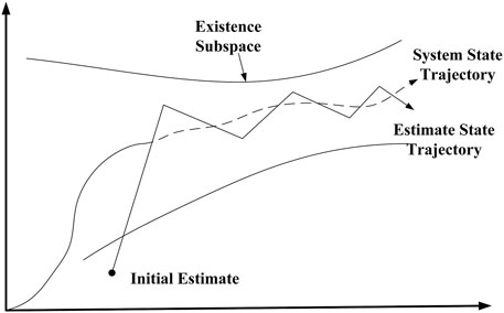
Figure 3. Structure of the smooth variable structure filter.

3.1 Model of the state-space model of distribution networks

The state-space model is used to estimate the state of the system based on the current state and the input signal. The state-space model is defined as shown in Eq. 2:

$\begin{array}{c}{\widehat{\mathit{x}}}_{\mathit{k}\left.+\mathbf{1}\right|\mathit{k}}=\mathit{f}\left({\mathit{x}}_{\mathit{k}}\right)+{\mathit{w}}_{\mathit{k}}\\ \begin{array}{c}{\mathit{z}}_{\mathit{k}}=\mathit{h}\left({\mathit{x}}_{\mathit{k}}\right)+{\mathit{v}}_{\mathit{k}}\\ \begin{array}{c}{\mathit{w}}_{\mathit{k}}\sim \left(\mathbf{0},{\mathit{Q}}_{\mathit{k}}\right)\\ {\mathit{v}}_{\mathit{k}}\sim \left(\mathbf{0},{\mathit{R}}_{\mathit{k}}\right)\end{array}\end{array}\end{array},(2)$

where $f$ and $h$ are the state-space model and measurement matrix of the power system, respectively. ${\widehat{x}}_{k\left.+1\right|k}$ is the predicted state estimate of the input system state vector, $x_k$ is the input system state vector, and $z_k$ is the observed state measurement. $w_k$ and $v_k$ are the state noise and measurement noise, respectively, which are usually assumed to follow Gaussian distributions with zero mean and covariance matrices in $\left(0,Q_k\right)$.

As shown in Eq. 2, in the modeling of the state-space model of distribution networks, the state vector $x\left(k\right)$ consists of the voltage magnitude $U_{N,k\left.+1\right|k}$ and voltage phase angle ${\delta }_{N,k\left.+1\right|k}$.The measurement vector $z_k$ consists of $P_{L,k},Q_{L,k},U_{N,k},{\delta }_{L,k},P_{pv,k\left.+1\right|k}$, which, respectively, represent real power, reactive power, voltage magnitude, phase angle, and PV power at the kth time sample.

With the Holt’s two-parameter linear exponential smoothing technique, $f\left(·\right)$ takes the following form (Wentao et al., 2019; Lujuan et al., 2020):

$\begin{array}{c}\mathit{f}\left({\mathit{x}}_{\mathit{k}}\right)={\mathit{s}}_{\mathit{k}}+{\mathit{u}}_{\mathit{k}}\\ {\mathit{s}}_{\mathit{k}}=\mathit{\alpha }{\mathit{x}}_{\mathit{k}}+\left(\mathbf{1}-\mathit{\alpha }\right){\widehat{\mathit{x}}}_{\mathit{k}+\mathbf{1}|\mathit{k}}\\ {\mathit{u}}_{\mathit{k}}=\mathit{\beta }\left({\mathit{s}}_{\mathit{k}}-{\mathit{s}}_{\mathit{k}-\mathbf{1}}\right)+\left(\mathbf{1}-\mathit{\beta }\right){\mathit{u}}_{\mathit{k}-\mathbf{1}}\end{array},(3)$

where $\alpha$ and $\beta$ are the constants in interval $\left(0,1\right)$ and ${\widehat{\mathit{x}}}_{\mathit{k}+\mathbf{1}|\mathit{k}}$ represents the predicted state vectors for k+1 time based on time k. The state forecasting function, Eq. 3, is used to predict ${\widehat{x}}_{k\left.+1\right|k}$.

The measurement function $h\left(.\right)$ as shown in the Eqs 4–7:

${\mathbf{P}}_N={\displaystyle {\sum }_{j=1}^{Load}}\left|{\mathbf{V}}_N\Vert {\mathbf{V}}_M\right|\left({\mathbf{G}}_{NM}\cos {\theta }_{NM}+{\mathbf{B}}_{nm}\sin {\theta }_{NM}\right),(4)$

${\mathbf{Q}}_N={\displaystyle {\sum }_{j=1}^N}\left|{\mathbf{V}}_N\Vert {\mathbf{V}}_M\right|\left({\mathbf{G}}_{NM}\sin {\theta }_{NM}-{\mathbf{B}}_{NM}\cos {\theta }_{NM}\right),(5)$

${\mathbf{P}}_{NM}={\mathbf{V}}_N^2\left({\mathbf{G}}_{gN}+{\mathbf{G}}_{sM}\right)-\left|{\mathbf{V}}_N\Vert {\mathbf{V}}_M\right|\left({\mathbf{G}}_{NM}\cos {\theta }_{NM}+{\mathbf{B}}_{NM}\sin {\theta }_{NM}\right),(6)$

${\mathbf{Q}}_{NM}=-{\mathbf{V}}_N^2\left({\mathbf{B}}_{gN}+{\mathbf{B}}_{sM}\right)-\left|{\mathbf{V}}_N\Vert {\mathbf{V}}_M\right|\left({\mathbf{G}}_{NM}\sin {\theta }_{NM}-{\mathbf{B}}_{NM}\cos {\theta }_{NM}\right),(7)$

where $\left|{\mathbf{V}}_N\right|$ is the voltage magnitude at node N and ${\theta }_{NM}$ is the voltage phase angle between nodes N and M. ${\mathbf{P}}_N$ and ${\mathbf{Q}}_N$ are injection real power and active power in node N, respectively, and ${\mathbf{P}}_{NM}$ and ${\mathbf{Q}}_{NM}$ are the flow of real power and active power between nodes N and M, respectively; all of these variables belong to variables $P_{L,k}$ and $Q_{L,k}$.

${\mathbf{G}}_{NM}$ and ${\mathbf{B}}_{NM}$ are the conductance and susceptance of the line between nodes N and M, respectively, and ${\mathbf{G}}_{gN}$ and ${\mathbf{B}}_{gN}$ are the conductance and susceptance, respectively.

For the predicted PV power in distribution networks, ${\mathbf{P}}_{NM}$ and ${\mathbf{P}}_N$ in PV nodes are deterministic. ${\mathbf{Q}}_N$ and ${\mathbf{Q}}_{NM}$ can be set to 0.

3.2 Prediction part

$\begin{array}{c}{\widehat{\mathit{x}}}_{\mathit{k}\left.+\mathbf{1}\right|\mathit{k}}=\mathit{A}{\widehat{\mathit{x}}}_{\mathit{k}|\mathit{k}}+{\mathit{w}}_{\mathit{k}}\\ {\widehat{\mathit{z}}}_{\mathit{k}|\mathit{k}}=\mathit{C}{\widehat{\mathit{x}}}_{\mathit{k}|\mathit{k}}+{\mathit{v}}_{\mathit{k}}\end{array},(8)$

$\begin{array}{c}{\left.\mathit{A}=\frac{\partial \mathit{f}\left({\mathit{x}}_{\mathit{k}}\right)}{\partial {\mathit{x}}_{\mathit{k}}}\right|}_{{\mathit{x}}_{\mathit{k}}={\stackrel{\sim }{\mathit{x}}}_{\mathit{k}|\mathit{k}}}\\ {\left.\mathit{C}=\frac{\partial \mathit{h}\left({\mathit{x}}_{\mathit{k}}\right)}{\partial {\mathit{x}}_{\mathit{k}}}\right|}_{{\mathit{x}}_{\mathit{k}}={\stackrel{\sim }{\mathit{x}}}_{\mathit{k}|\mathit{k}-\mathbf{1}}}\end{array}.(9)$

In Eqs 8, 9, ${\widehat{x}}_{k\left.+1\right|k}$ and ${\widehat{z}}_{k|k}$ are the predicted state estimate and measurement estimate, respectively. A and C are the Jacobian matrices of the nonlinear state function and measurement function (i.e., $f\left(.\right)$ and $h\left(.\right)$) linearized at the first-order Taylor series, respectively.

$P_{k\left.+1\right|k}$ is the state error covariance calculated using Eq. 1, and the measurement prediction value ${\widehat{z}}_{k\left.+1\right|k}$ is determined using Eqs 10, 11:

${\mathit{P}}_{\mathit{k}\left.+\mathbf{1}\right|\mathit{k}}=\mathit{A}{\mathit{P}}_{\mathit{k}|\mathit{k}}{\mathit{A}}^{\mathit{T}}+{\mathit{Q}}_{\mathit{k}},(10)$

${\widehat{\mathit{z}}}_{\mathit{k}\left.+\mathbf{1}\right|\mathit{k}}={\widehat{\mathit{C}}}_{\mathit{k}+\mathbf{1}}{\widehat{\mathit{x}}}_{\mathit{k}\left.+\mathbf{1}\right|\mathit{k}}+{\mathit{v}}_{\mathit{k}}.(11)$

The measurement estimation errors $e_{z,k+1\left|k\right.}$ and $e_{z,k+1\left|k\right.+1}$ are calculated using Eqs 12, 13:

${\mathit{e}}_{\mathit{z},\mathit{k}\left.+\mathbf{1}\right|\mathit{k}}={\mathit{z}}_{\mathit{k}+\mathbf{1}}-{\widehat{\mathit{z}}}_{\mathit{k}\left.+\mathbf{1}\right|\mathit{k}},(12)$

${\mathit{e}}_{\mathit{z},\mathit{k}\left.+\mathbf{1}\right|\mathit{k}+\mathbf{1}}={\mathit{z}}_{\mathit{k}+\mathbf{1}}-{\widehat{\mathit{z}}}_{\mathit{k}\left.+\mathbf{1}\right|\mathit{k}+\mathbf{1}}.(13)$

3.3 Measurement update correction part

The gain in SVSF is shown in Eq. 14. The convergence rate parameter $\gamma$ satisfies $0<\gamma <1$. The superscript “+” in C represents the pseudoinverse, $diag\left(\right)$ is a diagonalization symbol, and $\otimes$ represents the Schur product, which is the element-wise multiplication of matrices.

$\begin{array}{c}{\mathit{K}}_{\mathit{k}+\mathbf{1}}={\mathit{C}}_{\mathit{k}+\mathbf{1}}^{+}\mathit{d}\mathit{i}\mathit{a}\mathit{g}\left[\left(\left|{\mathit{e}}_{\mathit{z},\mathit{k}\left.+\mathbf{1}\right|\mathit{k}}\right|+\mathit{\gamma }\left|{\mathit{e}}_{\mathit{z},\mathit{k}|\mathit{k}}\right|\right)\otimes \mathit{s}\mathit{a}\mathit{t}\left({\stackrel{\mathbf{ˉ}}{\overline{\mathit{\psi }}}}_{\mathit{k}+\mathbf{1}}^{-\mathbf{1}},{\mathit{e}}_{\mathit{z},\mathit{k}\left.+\mathbf{1}\right|\mathit{k}}\right)\right]\mathit{d}\mathit{i}\mathit{a}\mathit{g}{\left({\mathit{e}}_{\mathit{z},\mathit{k}\left.+\mathbf{1}\right|\mathit{k}}\right)}^{-\mathbf{1}}\\ \mathit{s}\mathit{a}\mathit{t}\left(\mathit{a},\mathit{b}\right)=\left\{\begin{array}{cc}\frac{\mathit{a}}{\mathit{b}}& \left|\mathit{a}\right|\le \mathit{b}\\ \mathit{s}\mathit{i}\mathit{g}\mathit{n}\left(\mathit{a}\right)& \left|\mathit{a}\right|>\mathit{b}\end{array}\right\},\end{array}(14)$

where $\overline{\psi }$ is the diagonalization form that represents the boundary layer, which is obtained by taking partial derivatives of the error covariance in Eq. 15.

$\begin{array}{c}{\overline{\mathit{\psi }}}_{\mathbf{k}+\mathbf{1}}={\left[{\mathit{E}}_{\mathbf{k}+\mathbf{1}}^{-\mathbf{1}}{\mathit{C}}_{\mathbf{k}+\mathbf{1}}{\mathit{P}}_{\mathbf{k}+\mathbf{1}}{\mathit{C}}_{\mathbf{k}+\mathbf{1}}^{\mathit{T}}{\left({\mathit{P}}_{\mathit{k}\left.+\mathbf{1}\right|\mathit{k}}\right)}^{-\mathbf{1}}\right]}^{-\mathbf{1}}\\ {\mathit{E}}_{\mathbf{k}+\mathbf{1}}^{-\mathbf{1}}=\mathit{d}\mathit{i}\mathit{a}\mathit{g}\left(\left|{\mathit{e}}_{\mathit{z},\mathit{k}\left.+\mathbf{1}\right|\mathit{k}}\right|+\mathit{\gamma }\left|{\mathit{e}}_{\mathit{z},\mathit{k}|\mathit{k}}\right|\right)\end{array}.(15)$

The gain can update the state estimation value and can be obtained using Eq. 16.

${\widehat{\mathit{x}}}_{\mathit{k}\left.+\mathbf{1}\right|\mathit{k}+\mathbf{1}}={\widehat{\mathit{x}}}_{\mathit{k}\left.+\mathbf{1}\right|\mathit{k}}+{\mathit{K}}_{\mathit{k}+\mathbf{1}}{\mathit{e}}_{\mathit{z},\mathit{k}\left.+\mathbf{1}\right|\mathit{k}.}(16)$

The covariance matrix P is updated, and R is the covariance matrix of measurement noise in Eq. 17.

${\mathit{P}}_{\mathit{k}\left.+\mathbf{1}\right|\mathit{k}+\mathbf{1}}=\left(\mathit{I}-{\mathit{K}}_{\mathit{k}+\mathbf{1}}{\mathit{C}}_{\mathit{k}+\mathbf{1}}\right){\mathit{P}}_{\mathit{k}\left.+\mathbf{1}\right|\mathit{k}}{\left(\mathit{I}-{\mathit{K}}_{\mathit{k}+\mathbf{1}}{\mathit{C}}_{\mathit{k}+\mathbf{1}}\right)}^{\mathbf{T}}+{\mathit{K}}_{\mathit{k}+\mathbf{1}}\mathit{R}{\mathit{C}}_{\mathit{k}+\mathbf{1}}^{\mathbf{T}}.(17)$

By correcting and updating the covariance matrix at each time step, we can obtain more noise-resistant and accurate dynamic state estimates $\widehat{x}$.

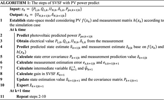
3.4 Improved dynamic state estimation method considering PV power prediction

In order to introduce photovoltaic power prediction into SVSF, when modeling the state-space model of the distribution network, the power of photovoltaics needs to be used as an input in parallel with the node voltage magnitude, voltage phase angle, and active power of the distribution network. The original state-space model is expressed in Eq. 2, where $x_k$ in the state-space model $f\left(x_k\right)$ represents the distribution network vectors $\left\{U_{N,k+1\left|k\right.},{\delta }_{N,k+1\left|k\right.}\right\}$. In this paper, when modeling in the state-space model considering the factors of photovoltaic prediction, the input vector $z_k$ of $h\left(z_k\right)$ includes $\left\{P_{L,k},Q_{L,k},U_{N,k},{\delta }_{L,k},P_{pv,k+1\left|k\right.}\right\}$. This establishes an association between the predicted state vector of distribution network and photovoltaic power prediction in the state-space model. When calculating measurement estimation errors $e_{z,k+1\left|k\right.}$ and $e_{z,k+1\left|k\right.+1}$ for the position of the measurement matrix where the photovoltaic node is located, the measurement error value is the difference value between the photovoltaic power prediction value and the actual photovoltaic power value, and the original calculation method is maintained for other load nodes. This realizes the real-time update of the system gain in the SVSF filtering of new energy power generation equipment. Algorithm 1 shows the steps of SVSF with PV power prediction. Figure 4 shows the comparison of the original SVSF and SVSF with PV power prediction.

Figure 4

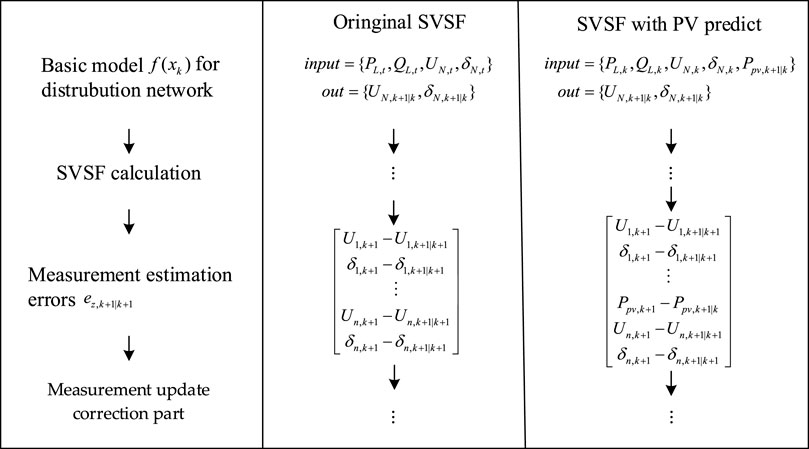
Figure 4. Difference between the original SVSF and SVSF with PV power prediction.

In this case, when modeling the state-space model of the distribution network, the photovoltaic output will become one of the powerful influencing factors affecting the output voltage magnitude and voltage phase angle. Therefore, the method of photovoltaic power prediction can also be connected to the Kalman filter; however, for the distribution network with many nodes with large fluctuations, SVSF can have stronger robustness by switching gains when it is impossible to model all possible situations. In the remainder of the paper, we will refer to the combination of SVSF and photovoltaic power prediction as “SVSF + Predict”.

4 Case study and evaluation

To verify the application effect of the SVSF used in the dynamic state estimation of the power system, this paper takes a 33-node distribution net example system (Baran and Wu, 1989) as the basis, and the system structure topology diagram is shown in Figure 5. The main power generation unit is at node 1, and photovoltaic power generation equipment is installed at nodes 18 and 22 to simulate the situation of system fluctuations after photovoltaic access. The power data of load nodes are adjusted according to the actual distribution network power data (Group, 2023) from 1 January to 31 December 2022, which is segmented to set in nodes’ power. In addition, the power generation and weather data of photovoltaic power generation equipment are converted based on the actual photovoltaic power generation equipment data from the dataset Ruiyuan, Z. (2021). The simulation training stage uses the tidal flow calculation results obtained by the MATPOWER toolbox in MATLAB. The method used for comparison in this paper is modified on the basis of UKF (Bhusal and Gautam, 2020) and SR-UKF (JJHu 1993, 2016). Each time section considers the acquisition time of the real measurement system (Liu Zhelin et al., 2021), and the time step of each section is 5 min, with a total of 3,000 times and a total of 250 h.

Figure 5

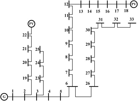
Figure 5. Topology of 33-node distribution network case.

Under normal operation, the distribution network is usually quite stable, with the voltage magnitude maximum fluctuation being only 2%, making it difficult to evaluate the effectiveness of dynamic state estimation solely based on the percentage difference in amplitude. When assessing the accuracy between the predicted and actual values, it is common to use RMSE, MAPE, and mean absolute error (MAE) to measure the deviation between the estimated and true values. RMSE is calculated using Eq. 18, which is the square root of the mean squared error between the predicted and actual values. A smaller RMSE indicates a smaller absolute error between the predicted and actual values. MAPE is calculated using Eq. 19, which is the mean of all absolute percentage errors between the predicted and actual values. A smaller MAPE indicates a smaller relative error between the predicted and actual values under the same scale. MAE is calculated using Eq. 20. It is similar to MAPE, but it is a better representation of error. MAPE and MAE are metrics used to measure the performance of dynamic state estimation:

$\mathit{R}\mathit{M}\mathit{S}\mathit{E}\left(\mathit{k}\right)=\sqrt{\frac{\mathbf{1}}{\mathit{N}}{\displaystyle {\sum }_{\mathit{i}=\mathbf{1}}^{\mathit{N}}}{\left({\widehat{\mathit{y}}}_{\mathit{k},\mathit{i}}-{\mathit{y}}_{\mathit{k},\mathit{i}}\right)}^{\mathbf{2}}},(18)$

$\mathit{M}\mathit{A}\mathit{P}\mathit{E}\left(\mathit{k}\right)=\frac{\mathbf{1}}{\mathit{N}}{\displaystyle {\sum }_{\mathit{i}=\mathbf{1}}^{\mathit{N}-\mathbf{1}}}\frac{\left|{\widehat{\mathit{y}}}_{\mathit{k},\mathit{i}}-{\mathit{y}}_{\mathit{k},\mathit{i}}\right|}{{\mathit{y}}_{\mathit{k},\mathit{i}}},(19)$

$\mathit{M}\mathit{A}\mathit{E}\left(\mathit{k}\right)=\frac{\mathbf{1}}{\mathit{N}}{\displaystyle {\sum }_{\mathit{i}=\mathbf{1}}^{\mathit{N}}}|{\widehat{\mathit{y}}}_{\mathit{k},\mathit{i}}-{\mathit{y}}_{\mathit{k},\mathit{i}}|.(20)$

Here, $k$ represents the node number, $N$ represents the length of the entire prediction sequence, and $i$ is the time of calculation. ${\widehat{y}}_{k,i}$ represents the predicted value, and $y_{k,i}$ is the actual value.

4.1 Dynamic state estimation in distribution networks

Node 16 is a node located at the end of the distribution system, which is far from the main stable generator at node 1 but depends on the PV installation node located at 18. Its voltage magnitude and phase angle are affected by normal load fluctuations and PV power, and the abnormal fluctuations of its magnitude and phase angle are more severe than those of the conventional node, represented by node 24, as described below. Under this node, UKF and SVSF are comparable in the accuracy of magnitude prediction, while in SVSF + Predict, its MAPE value is only half of that of the above two methods. Node 24 is the node located alone in the branch, which is closer to both the generator and PV nodes. In most cases, at this node, the performance of the three methods is closer. However, from the macroscopic statistics of the data over a long period of time, it can be obtained that SVSF + Predict still achieves better results compared to the other two methods, and its RMSE, MAPE, and MAE values are shown in Table 3. Figures 6, 7 show the estimation error of voltage magnitude and voltage phase angle plots for nodes 16 and 24.

Table 3

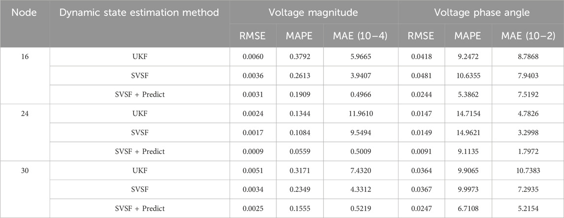
Table 3. RMSE, MAPE, and MAE values of voltage magnitude and voltage phase angle for some nodes.

Figure 6

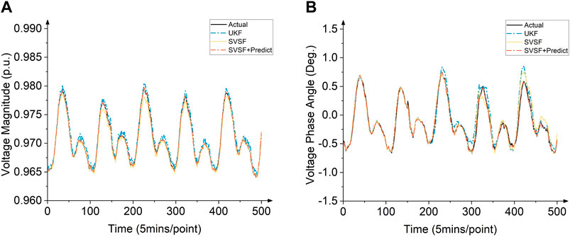
Figure 6. (A) Estimation error of voltage magnitude for node 16. (B) Estimation error of voltage phase angle for node 16.

Figure 7

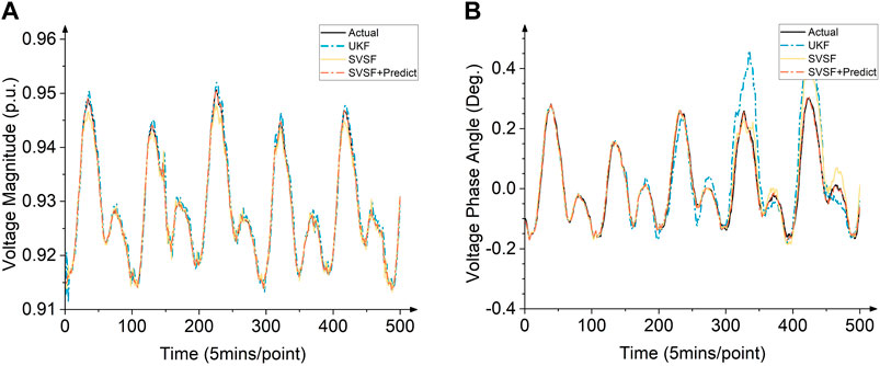
Figure 7. (A) Estimation error of voltage magnitude for node 24. (B) Estimation error of voltage phase angle for node 24.

The dynamic state estimation results of voltage magnitude and voltage phase angle are provided in Table 3. Active power is considered the PV prediction factor when establishing the state-space model In addition, the influence of active power on voltage magnitude is much smaller than that on voltage phase angle in the distribution network. Therefore, the PV power prediction is more closely related to the estimated voltage phase angle. In the 16 nodes that are near the photovoltaic generation, the addition of photovoltaic power prediction more effectively strengthens the dynamic state estimation accuracy of the node.

In comparison with the dynamic state estimation results of voltage magnitude and voltage phase angle in Table 3, active power is considered the additional factor when establishing the state-space model. In addition, the influence of active power on voltage magnitude is much smaller than that on voltage phase angle in the distribution network. Therefore, the PV power prediction is more closely related to the changes in voltage phase angle. As a result, in the 33-node case, the improvement in the voltage phase angle of the dynamic state estimation is more effective than that in the voltage magnitude, which can be derived from RMSE and MAPE on node 16.

Figure 8 shows the RMSE and MAPE of voltage magnitude and voltage phase angle at all 33 nodes. At almost the majority of the nodes, SVSF + Predict achieves better prediction accuracy than SVSF or UKF. This figure is roughly divided into three segments by branches in distribution networks: nodes 2–18, 20–25, and 26–33. The worst prediction value among the three methods is located at node 18, which is not only far from the generator node but also the PV node, and thus, the prediction is mainly affected by the PV power; without the assistance of PV power prediction, the prediction results of both UKF and SVSF at this node show a more serious bias. In contrast, in the combination of PV power prediction, MAPE is decreased by 50%. Second, among nodes 19–33, node 33 is the node with the largest error. This node is located far from the initial generation node and at the end of the line, and in SVSF + Predict, its error increases more slowly compared to the other two methods, and better results are achieved compared to that without the assistance of PV power prediction.

Figure 8

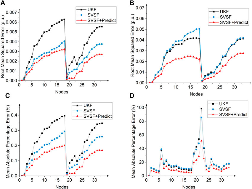
Figure 8. (A) RMSE of voltage magnitude at all 33 nodes. (B) RMSE of voltage phase angle at all 33 nodes. (C) MAPE of voltage magnitude at all 33 nodes. (D) MAPE of voltage phase angle at all 33 nodes.

In general, in the nodes near the photovoltaic power generation, such as node 16, the addition of photovoltaic power forecasting more effectively strengthens the dynamic state estimation accuracy of the node. However, for nodes with relatively stable operation that are not seriously affected by PV fluctuations, like nodes 24 and 30, the improvement in the estimation accuracy of the proposed method is not as obvious as that of node 16, and it only improves the SVSF’s performance on these nodes to a small extent.

4.2 Dynamic state estimation in noise interference

For the case study under noise interference, SCADA is configured in each branch of the distribution network, and PMU is configured in nodes 2, 6, and 12. The standard deviation of measurement error of branch power data collected by SCADA is set to be 0.02, and the standard deviation of measurement error of voltage magnitude and phase angle collected by PMU is set to be 0.005 and 0.002, respectively.

The results of dynamic state estimation under noise interference are shown in Table 4. Under the interference of noise, the dynamic state estimation effect of UKF, SRUKF, and the proposed method is affected. For nodes such as node 16 that are close to the photovoltaic setting branch, the predicted photovoltaic power in the simulation is still accurate. Therefore, under the interference of noise, the dynamic state results of the proposed method in branches near the influence are not obvious, and they have a strong anti-interference ability. For nodes 24 and 30, due to noise interference, the dynamic state estimation results have a greater loss of accuracy than the results without noise interference. The variation in error value of dynamic state estimates for phase angles with larger original magnitudes is more obvious. However, in general, the RMSE value of dynamic state estimation proves that it is still in the valid range under noise interference.

Table 4

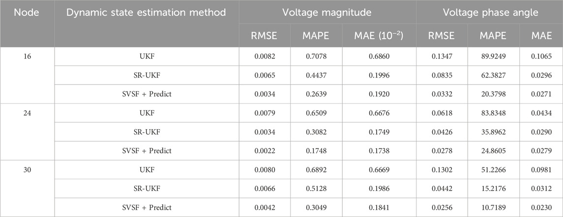
Table 4. RMSE, MAPE, and MAE values of voltage magnitude and voltage phase angle for some nodes under noise interference.

5 Conclusion

To address the inaccuracy associated with the existing dynamic state estimation method based on the Kalman filter, this paper proposed an SVSF-based dynamic state estimation method with consideration of PV power prediction. Compared with the traditional UKF algorithm, this method offers greater advantages in accuracy and robustness. The proposed method can more effectively strengthen the dynamic state estimation accuracy of the node near the photovoltaic power generation. In addition, under the interference of noise, the proposed method has a strong anti-interference ability.

1. Improved dynamic state estimation based on SVSF considering PV power prediction is characterized by introducing photovoltaic power prediction when modeling the state-space model of the distribution network and relying on the new factor of photovoltaic output prediction in pre-modeling to model the impact of photovoltaic output on the dynamic state estimation of the distribution network, alleviating the uncertainty caused by photovoltaic fluctuations.

2. Improved dynamic state estimation based on SVSF considering PV power prediction uses noise information and error information, uses SVSF gain to switch on both sides of the existing subspace, and forces $\widehat{x}$ to the vicinity of the existing subspace, thereby correcting the estimated value to the vicinity of the true value.

3. Improved dynamic state estimation based on SVSF considering PV power prediction also has strong filtering and estimation performance when the state-space model is not accurate. In addition, this paper also verifies that under the condition of large fluctuations and noise interference in the distribution network, SVSF can more effectively suppress the divergence problem caused by model inaccuracy compared to UKF.

At present, the research considers photovoltaics as a representative of renewable energy. The next step is to study the prediction of other renewable energy sources in combination with SVSF to improve the proposed method.

Data availability statement

The raw data supporting the conclusions of this article will be made available by the authors, without undue reservation.

Author contributions

HZ: conceptualization, methodology, and writing–original draft. XC: methodology and writing–original draft. JW: methodology and writing–original draft. RM: investigation and writing–original draft. RF: data curation and writing–review and editing. TW: software and writing–review and editing. JS: software and writing–review and editing. GX: writing–review and editing.

Funding

The author(s) declare that financial support was received for the research, authorship, and/or publication of this article. This work was supported by State Grid Shanxi Electric Power Company Science and Technology Project Research (52053023000V).

Conflict of interest

The authors declare that this study received funding from State Grid Shanxi Electric Power Company. The funder had the following involvement: study design, data collection and analysis, methodology, investigation, resources and preparation of the manuscript.

Authors HZ, XC, JW, RM, RF, TW, and JS were employed by State Grid Shanxi Electric Power Company.

The remaining author declares that the research was conducted in the absence of any commercial or financial relationships that could be construed as a potential conflict of interest.

Publisher’s note

All claims expressed in this article are solely those of the authors and do not necessarily represent those of their affiliated organizations, or those of the publisher, the editors, and the reviewers. Any product that may be evaluated in this article, or claim that may be made by its manufacturer, is not guaranteed or endorsed by the publisher.

References

Aljdaeh, E., Kamwa, I., Hammad, W., Abuashour, M. I., Sweidan, T. E., Khalid, H. M., et al. (2021). Performance enhancement of self-cleaning hydrophobic nanocoated photovoltaic panels in a dusty environment. Energies 14 (20), 6800. doi:10.3390/en14206800

CrossRef Full Text | Google Scholar

Baran, M. E., and Wu, F. F. (1989). Network reconfiguration in distribution systems for loss reduction and load balancing. IEEE Trans. Power Deliv. 4 (2), 1401–1407. doi:10.1109/61.25627

CrossRef Full Text | Google Scholar

Bhusal, N., and Gautam, M. (2020). Power system dynamic state estimation using extended and unscented Kalman filters. arXiv preprint arXiv:2012.06069.

Google Scholar

Gadsden, S. A., and Habibi, S. R. (2013). A new robust filtering strategy for linear systems. J. Dyn. Syst. Meas. Control 135 (1), 014503. doi:10.1115/1.4006628

CrossRef Full Text | Google Scholar

Group, E. (2023). Elia open data portal. Available at: https://opendata.elia.be/pages/home/(Accessed December 10, 2023).

Google Scholar

Guanghua, Z., Linghao, Z., Feng, L., Xinqiang, L., Na, F., and Shasha, D. (2022). State estimation for dynamic systems with higher-order autoregressive moving average non-Gaussian noise. Front. Energy Res. 10. doi:10.3389/fenrg.2022.990267

CrossRef Full Text | Google Scholar

Habibi (2007). The smooth variable structure filter. Proc. IEEE 95 (5), 1026–1059. doi:10.1109/jproc.2007.893255

CrossRef Full Text | Google Scholar

Habibi, S. R., and Burton, R. (2003). The variable structure filter. J. Dyn. Syst. Meas. Control 125 (3), 287–293. doi:10.1115/1.1590682

CrossRef Full Text | Google Scholar

Hammad, W., Sweidan, T. E. O., Abuashour, M. I., Khalid, H. M., and Muyeen, S. (2021). Thermal management of grid-tied PV system: a novel active and passive cooling design-based approach. IET Renew. Power Gener. 15 (12), 2715–2725. doi:10.1049/rpg2.12197

CrossRef Full Text | Google Scholar

Haykin, S., and Arasaratnam, I. (2009). Cubature kalman filters. IEEE Trans. Automatic Control 54 (6), 1254–1269. doi:10.1109/tac.2009.2019800

CrossRef Full Text | Google Scholar

Jiawei, W., Keman, L., Feng, W., Zizhao, W., Linjun, S., and Yang, L. (2023). Improved unscented Kalman filter based interval dynamic state estimation of active distribution network considering uncertainty of photovoltaic and load. Front. Energy Res. 10. doi:10.3389/fenrg.2022.1054162

CrossRef Full Text | Google Scholar

Jinliang, Z., Ziyi, L., and Tao, C. (2023). Interval prediction of ultra-short-term photovoltaic power based on a hybrid model. Electr. Power Syst. Res. 216, 109035. doi:10.1016/j.epsr.2022.109035

CrossRef Full Text | Google Scholar

Jjhu1993 (2016). Square root unscented kalman filter using MATLAB. Available at: https://github.com/JJHu1993/sr-ukf (Accessed November 7, 2023).

Google Scholar

Keddouda, A., Ihaddadene, R., Boukhari, A., Atia, A., Arıcı, M., Lebbihiat, N., et al. (2023). Solar photovoltaic power prediction using artificial neural network and multiple regression considering ambient and operating conditions. Energy Convers. Manag. 288, 117186. doi:10.1016/j.enconman.2023.117186

CrossRef Full Text | Google Scholar

Khalid, H. M., Rafique, Z., Muyeen, S., Raqeeb, A., Said, Z., Saidur, R., et al. (2023). Dust accumulation and aggregation on PV panels: an integrated survey on impacts, mathematical models, cleaning mechanisms, and possible sustainable solution. Sol. Energy 251, 261–285. doi:10.1016/j.solener.2023.01.010

CrossRef Full Text | Google Scholar

Liu Zhelin, W. C., Peng, Li, Yu, H., Li, Y., and Peng, L. (2021). State estimation and application of distribution network based on multi-source measurement data fusion. Chin. J. Electr. Eng. 41, 2605–2615. doi:10.13334/j.0258-8013.pcsee.201416

CrossRef Full Text | Google Scholar

Lujuan, D., Badong, C., Shiyuan, W., Wentao, M., and Pengju, R. (2020). Robust power system state estimation with minimum error entropy unscented kalman filter. IEEE Trans. Instrum. Meas. 69 (11), 8797–8808. doi:10.1109/tim.2020.2999757

CrossRef Full Text | Google Scholar

Lupeng, C., Jian, L., Zhongmei, P., and Zhihua, Z. (2023). Static parameter estimation and testability analysis of distribution lines based on multi-source measurement information. Front. Energy Res. 11. doi:10.3389/fenrg.2023.1249782

CrossRef Full Text | Google Scholar

Mandal, J. K., Sinha, A. K., and Roy, L. (1995). Incorporating nonlinearities of measurement function in power system dynamic state estimation. IEE Proc. 142 (3), 289–296. doi:10.1049/ip-gtd:19951715

CrossRef Full Text | Google Scholar

Polasek, T., and Čadík, M. (2023). Predicting photovoltaic power production using high-uncertainty weather forecasts. Appl. Energy 339, 120989. doi:10.1016/j.apenergy.2023.120989

CrossRef Full Text | Google Scholar

Ruiyuan, Z. (2021). ST PV forecast. Available at: https://ieee-dataport.org/documents/st-pv-forecast (Accessed December 12, 2023).

Google Scholar

Sharma, A., Srivastava, S. C., and Chakrabarti, S. (2017). A cubature kalman filter based power system dynamic state estimator. IEEE Trans. Instrum. Meas. 66 (8), 2036–2045. doi:10.1109/tim.2017.2677698

CrossRef Full Text | Google Scholar

Wang, S., Gao, W., and Meliopoulos, A. P. S. (2012). An alternative method for power system dynamic state estimation based on unscented transform. IEEE Trans. Power Syst. 27 (2), 942–950. doi:10.1109/tpwrs.2011.2175255

CrossRef Full Text | Google Scholar

Wentao, M., Jinzhe, Q., Xinghua, L., Gaoxi, X., Jiandong, D., and Badong, C. (2019). Unscented kalman filter with generalized correntropy loss for robust power system forecasting-aided state estimation. IEEE Trans. Industrial Inf. 15 (11), 6091–6100. doi:10.1109/tii.2019.2917940

CrossRef Full Text | Google Scholar

Zhao, Y. (2015). Research and application on BP neural network algorithm. Xi’an, China: Atlantis Press, 1444–1447.

Google Scholar