
95% of researchers rate our articles as excellent or good
Learn more about the work of our research integrity team to safeguard the quality of each article we publish.
Find out more
ORIGINAL RESEARCH article
Front. Energy Res. , 29 July 2024
Sec. Sustainable Energy Systems
Volume 12 - 2024 | https://doi.org/10.3389/fenrg.2024.1418302
This article is part of the Research Topic Optimal Scheduling of Demand Response Resources In Energy Markets For High Trading Revenue and Low Carbon Emissions View all 34 articles
 Jiaji Liu*
 Peng Di
The high proportion of new energy into the power grid leads to a significant uneven distribution trend of the inertia of the power grid, which seriously affects the safe and stable operation of the power grid. It is urgent to carry out the inertia evaluation of the new energy power system. In view of the insufficient accuracy of the equivalent inertia evaluation method of a single inertia center in evaluating large-scale power systems, this paper first proposed the equivalent inertia evaluation method of new energy power system in the region, and proposed the evaluation index of network area inertia to reveal the weak inertia network area. Secondly, for the inertia evaluation of new energy power system nodes, monitoring devices should be installed at each bus node. As the system construction cost is too high, a node inertia evaluation model of new energy power system is established to reduce the number of monitoring devices installed. Finally, in view of the unclear basis and inaccurate location of the frequency monitoring node selection model in the evaluation of equivalent inertia, a correlation model of equivalent inertia and node inertia is established to characterize the correlation between any node inertia and system equivalent inertia in the system. The consistency of the position of the equivalent inertia evaluation frequency monitoring node and the maximum inertia node of the system was derived, and the accuracy of the maximum inertia node as a frequency monitoring node was verified by the inertia center method and the frequency center method.
With the proposal of the “carbon peak and carbon neutrality” strategy and the goal of constructing a new energy-based power system, traditional power systems are gradually transitioning to new energy power systems (Zhou et al., 2018; State Administration for Market Regulation, 2019; ENTSO-E, 2020). However, as a high proportion of new energy sources are integrated into the grid through power electronic devices, the weak inertia and low damping characteristics of new energy units are becoming increasingly prominent (Chen et al., 2017; Wen et al., 2020; Zhao et al., 2022). At the same time, the proportion of synchronous generators with large inertia is gradually decreasing, leading to a significant decrease in system inertia levels and posing a serious threat to system stability (Zhu et al., 2018; Jia et al., 2023; Tang et al., 2024).
Therefore, from the perspective of power system stability, evaluating the inertia level of high-proportion new energy power systems is of great significance (Lu et al., 2023; Li et al., 2024). Currently, scholars at home and abroad have conducted some work on the evaluation of inertia levels in high-proportion new energy power systems, mainly focusing on two aspects: system equivalent inertia evaluation and node inertia evaluation. Literature (Li et al., 2021; Li et al., 2020) elucidates methods for evaluating system equivalent inertia. The deficiency of literature (Li et al., 2021) lies in not clearly specifying the installation positions and reasons for frequency change rate and power change detection devices, while literature (Li et al., 2020) explicitly states that the installation position of detection devices should be the bus node referred to as the inertia centroid and provides a method for determining the inertia centroid based on network electrical distances and generator inertia time constants, but does not prove that the inertia centroid node is the most suitable for conducting system equivalent inertia evaluation, nor does it define and calculate the electrical distance. Literature (Liu et al., 2020; Liu, 2021; Liu et al., 2021) proposes a node inertia calculation model based on grid structural parameters, but there are unclear and ambiguous definitions and explanations of the synchronous power coefficient (e.g., Bjk is the reactance shrinking to the potential node j inside the generator and fault node k"), and it does not provide its calculation method. Literature (Xiao et al., 2020) uses frequency center, while literature (Liu et al., 2020) uses the frequency average of several measurement points in the region to replace the inertia center, which is insufficiently based on literature (Zeng, 2020; Zeng and Zhang, 2020). To evaluate the system node inertia, power-frequency detection devices (such as PMUs) need to be installed at all busbars, which greatly increases costs.
In fact, due to the rapid development of new energy generation and the uneven distribution of system inertia after new energy integration due to natural resource constraints, the traditional single inertia center equivalent inertia evaluation scheme cannot identify weak inertia links caused by new energy integration. In view of this, this paper firstly proposes a grid area equivalent inertia evaluation method based on the position of synchronous generators and proposes grid area equivalent inertia evaluation indicators. The scheme is applied to the evaluation of grid area equivalent inertia in a certain power grid in China, revealing the level of grid area equivalent inertia before and after the integration of new energy sources and identifying weak inertia grid areas. Secondly, considering that grid area equivalent inertia evaluation can only reflect the overall inertia level of the entire grid area and cannot specifically reveal the distribution law of inertia within the grid area and the weak inertia nodes, based on this, this paper proposes a power system node inertia evaluation scheme based on grid structural parameters and synchronous generator power factors to evaluate the overall inertia level of the entire system, analyze the impact of new energy integration on the distribution law of system inertia, and identify weak inertia links within each grid area. Finally, aiming at the problem of unclear position of inertia evaluation nodes (frequency monitoring nodes) in inertia calculation methods, this paper, combined with the research on node inertia and equivalent inertia, starts from node inertia, analyzes the quantitative relationship between each node inertia and system equivalent inertia, and determines the power-frequency characteristics and specific positions of frequency monitoring nodes to provide theoretical support for selecting inertia evaluation nodes when evaluating system equivalent inertia through inertia calculation methods, reduce the number of PMU installations, and reduce costs. This paper uses BPA data from a certain power grid in China for simulation verification, and the simulation environment is MATLAB.
In studies evaluating the equivalent inertia of power systems, the inertia statistical method based on unit switch data reads the unit switch status from the SCADA system. It combines the inertia time constant of the unit and calculates the inertia of the unit in the access system by weighting the inertia of the unit according to the unit’s capacity. This method obtains unit switch data, including the on and off states of the unit, as well as the unit’s capacity information. Based on the unit’s inertia time constant, the inertia characteristics of the unit can be determined. Then, based on the weight of the unit’s capacity, the inertia of the units connected to the system is weighted and added to obtain the system’s inertia. The equivalent inertia time constant of the system can be calculated using the following formula:
In the formula, where Hsys represents the equivalent inertia time constant of the system, Si represents the capacity of the ith unit, Hi represents the inertia time constant of the ith unit, and (n) represents the number of units.
In the power system, new energy is limited by generation resources, resulting in uneven distribution within the system. As the scale of new energy increases gradually, the uneven distribution of system inertia becomes more prominent. Therefore, the equivalent inertia evaluated by inertia statistical methods has limitations, and it is necessary to consider dividing the system into zones based on the distribution characteristics of system inertia.
For a power system, the core factors affecting the inertia at a certain location are the inertia of each generator unit within the system and the electrical distance from that location to the generators. In actual power systems, power plants are often located within or near cities, resulting in shorter electrical distances and stronger inertia influence within or near urban areas. Conversely, areas farther from cities experience weaker inertia influence from power plants within or near those cities. Therefore, dividing the power system into network zones based on the geographical locations of synchronous generators yields:
In the equation, HsysJ represents the equivalent inertia constant of network zone J, where Hi and Si denote the inertia constant and capacity of traditional generator units within network zone J, and Sj represents the capacity of new energy generator units within network zone J.
According to the division of grid areas based on the geographical location of synchronous generators in Section 1.1, and after calculating the equivalent inertia HsysJ of each grid area using Eq. 2 by summing up the capacities of synchronous generators and new energy units within the grid area, a quantitative evaluation index for inertia in a certain power grid in China is constructed as follows (ENOT, 2018; Sun et al., 2020):
(1) When HsysJ > 4 s, it is considered that the inertia in grid zone J of the power grid in China is sufficient.
(2) When HsysJ < 2 s, Considering that the inertia of network zone J in a certain Chinese power grid is insufficient, leading to poor dynamic frequency response after disturbances and a higher risk of instability, it is recommended to implement additional inertia compensation at the connection points of new energy generator units within the network zone.
(3) When 2 < HsysJ < 4 s, the inertia in grid zone J of the power grid in China is within the normal range. The priority of inertia compensation in this case is lower, and priority should be given to compensating grid areas with equivalent inertia time constants less than 2 s.
Based on the assessment and evaluation criteria of network zone equivalent inertia, combined with the generator parameters of the power system, the equivalent inertia levels of each network zone can be evaluated. Weak inertia network zones can be identified, and efforts can be made to improve the inertia of network zones with equivalent inertia constants less than 2s to enhance the overall stability of the power system.
In Section 1, we proposed an assessment of the equivalent inertia of new energy power system network zones based on the inertia statistical method and put forward inertia evaluation indicators and evaluation criteria. This approach can evaluate the level of equivalent inertia in various network zones of the actual system and identify weak inertia network zones based on the evaluation indicators. However, the evaluation of network zone equivalent inertia cannot reveal the spatial distribution of inertia within the network zone or specific weak inertia nodes. Therefore, to accurately identify weak inertia nodes within the network zone and compensate for inertia to enhance network zone stability, further research is needed on node inertia assessment in weak inertia network zones.
Different from the study of system equivalent inertia assessment, which assumes uniform inertia distribution and simulates the entire system as a single synchronous generator, with the increasing penetration of new energy generator units, the system inertia distribution exhibits significant spatial non-uniformity. Consequently, when different nodes experience power disturbances, the initial rate of frequency change in the system varies. Therefore, based on system equivalent inertia, system power, and frequency change, we define node inertia.
The inertia of node k refers to the ratio of the magnitude of the disturbance power at node k to the initial rate of frequency change at node k when a power disturbance occurs at node k. It can be expressed as follows:
In the equation
It is worth noting that passive nodes themselves do not possess inertia. Node inertia represents the dynamic response of power-frequency characteristics at the node location after disturbances occur in the system.
There are two main methods for calculating the nodal inertia of complex power systems. The first method requires the installation of power-frequency monitoring devices, such as phase measurement units, at the grid nodes to collect the system node power change and frequency change rate after the disturbance. This method is easy to operate, intuitive and easy to understand, but requires the installation of monitoring devices at each node, which is costly. The second method is to predict the amount of power change and frequency change rate at each node after the perturbation based on the grid structure parameters and generator set parameters, which is less costly but introduces a certain error. Therefore, considering that the power system is unable to install detection devices at all nodes, and that the grid area structure parameters and generator dynamic parameters are easy to collect, the two methods are synthesized to carry out the assessment of system node inertia level.
As can be seen from Eq. 3, calculating the node inertia according to the structural parameters of the power system and generator parameters, it is necessary to establish the power and frequency correspondence between the generator node and the network node after the perturbation, respectively, and therefore the frequency and power correlation model of the system after the perturbation is proposed as follows.
In order to simplify the calculation difficulty of the model, it is assumed that the phase angle difference between the nodes is small after the system is disturbed, and the nodes of the system work near the rated voltage. At the same time, in order to characterize the weak inertia characteristics of the new energy unit and simplify the calculation difficulty, the new energy unit is replaced by the equivalent synchronous generator set with the same capacity and smaller inertia, ignoring the damping and non-synchronous power, and the load is regarded as the grounded conductor.
As can be seen in Figure 1, the system has n network nodes and m generator nodes. Nodes n+1, n+2, ., n + m are the internal voltage nodes of the generators after transient reactance. The node voltage equation is:
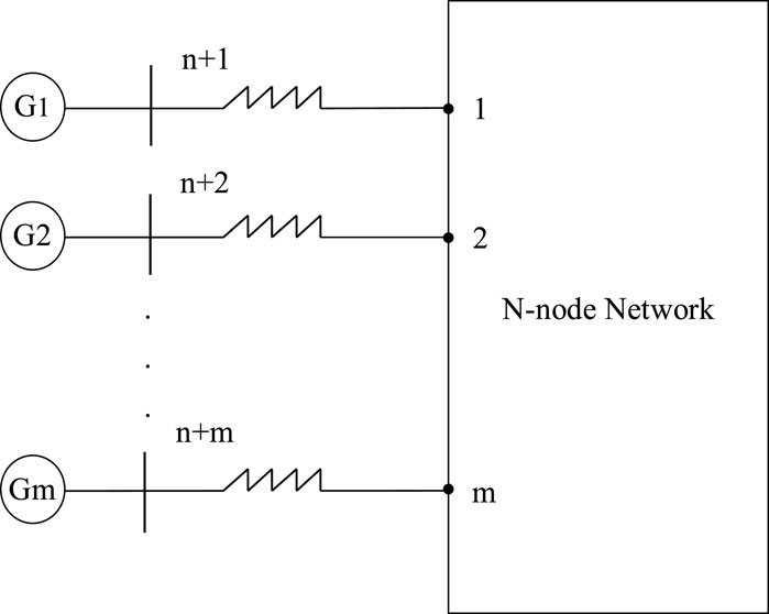
Figure 1. Equivalent diagram of multi-machine network in power system.
In the equation,
After equating the load to grounding admittance and keeping it constant, supplementing the load equivalent admittance matrix
Let
Eq. 6 yields:
In the equation,
Combining Eqs 3, 6, the relationship between the frequency of network nodes and the frequency of internal potential nodes of the generators is given by (Liu et al., 2021):
In the equation,
The active power output of synchronous generator i is:
In the equation:
In the equation:
In the actual system, the conductance is far less than the susceptance, so the effect of conductance is ignored. Therefore, when the power disturbance occurs at a node k of the system, the load effect is ignored, and the synchronous power coefficient Dik of generator i at node k is expressed as:
In the equation:
As can be obtained from formula (10), the power compensation of the generator set system of m station to node k is:
Therefore, the change of disturbed power
As can be seen from Eq. 13, when the disturbance
In Eq. 11,
According to Eq. 6, the transfer admittance matrix between the potential node and the network node in the generator is (see Supplementary Appendix):
In the equation:
From Eq. 15, the transfer admittance matrix and the association matrix can be established as:
As can be seen from Eq. 16, ignoring the influence of conductance, the correlation matrix between Eq. 11 synchronous power coefficient transfer admittance
Where:
Since each node of the system works near the rated voltage, the phase Angle
The inertia time constant of the network node k is expressed as:
The core of the equivalent inertia assessment calculation is to identify the equivalent inertia assessment node (also known as frequency monitoring node) of the system, where PMUs or other measurement devices can be installed to measure the power and frequency variations at that node after disturbances. However, currently there is a lack of mathematical basis for selecting the inertia assessment node. Therefore, from the perspective of inertia assessment, this study investigates the characteristics required for the inertia assessment node and how to accurately locate the frequency monitoring node in the system.
In the system, there are m synchronous generators, where the rotor swing equation for the ith generator (neglecting damping) is:
In the equation,
The evaluation formula for the equivalent inertia of the system is as follows:
In the equation,
Typically,
The inertia time constant of system node k, the inertia time constant of the system’s center of inertia
The equation states that
From Eq. 25, it can be observed that under the condition of Eq. 26, the inertial time constant of the node inertia in the power system is related to the equivalent inertia constant of the system and the inertial constant of the system inertia center as follows:
In practical systems, node positions are fixed and exhibit a discrete distribution in space, so they generally cannot strictly satisfy Eq. 26. In this case, the relationship between the inertial time constants of the system inertia center node and the maximum inertia node is as follows:
Under the influence of the same disturbance, the frequency deviation at node k in the system and the frequency deviation rate at the inertia center COI satisfy the following relationship:
Combining the above, when evaluating the system equivalent inertia using the inertia calculation method, the selected inertia evaluation node is the system’s maximum inertia node. Under the condition of satisfying Eq. 26, the inertia evaluation node coincides with the system inertia center, and the inertia detected by the evaluation node equals the system’s equivalent inertia. However, in actual systems, due to the discrete nature of power system bus nodes, Eq. 26 cannot be strictly satisfied. Therefore, the inertia detected by the system inertia evaluation node (i.e., the maximum inertia node) should be slightly less than the system’s equivalent inertia. As per Eqs 29, 30, it can be observed that the difference between the frequency deviation rate at the system inertia evaluation node and the frequency deviation rate at the inertia center is minimized.
In order to investigate the impact of integrating new energy into a certain power system in China on the level of equivalent inertia, and to demonstrate the trend of weak inertia in the system, this study adopts the method of sectional equivalent inertia assessment described in Section 1. The power grid is divided into n grid areas based on geographical location, and the level of equivalent inertia in each grid area of the power grid before and after the integration of new energy is evaluated. The specific steps are as follows:
(1) Data preprocessing: Organize the generator parameters and grid structure parameters in the BPA data of a certain power grid in China according to n grid areas, and find out the corresponding generator parameters and grid structure parameters for each grid area.
(2) Differentiation and statistics of generator inertia and capacity: Distinguish between traditional generator units and new energy generator units in each grid area based on dynamic parameters of generators (dynamic parameter cards in generator dynamic data correspond to different generator units), where the inertia of traditional generator units i within each grid area Hi is determined using the data on the nameplate of the generator, and the inertia of new energy units j Hj is set to 0.
(3) Calculation of equivalent inertia in each grid area before the integration of new energy: Calculate the level of equivalent inertia in each grid area before the integration of new energy by combining the inertia constants Hi and corresponding capacities Si of traditional generator units within each grid area according to Eq. 2.
(4) Calculation of equivalent inertia in each grid area after the integration of new energy: Calculate the level of equivalent inertia in each grid area after the integration of new energy by combining the inertia constants Hi and corresponding capacities Si of traditional generator units within each grid area and the capacity Sj of new energy units j according to Eq. 2.
Through the above process, the power system of a certain power grid in China is analyzed, and the system inertia level in each grid area before the large-scale integration of new energy is calculated. The results are visualized in Figure 2. The results show that before the integration of new energy, the lowest equivalent inertia level in region C of the power grid is 1.55s, while the highest equivalent inertia level in region D is 5.25s.
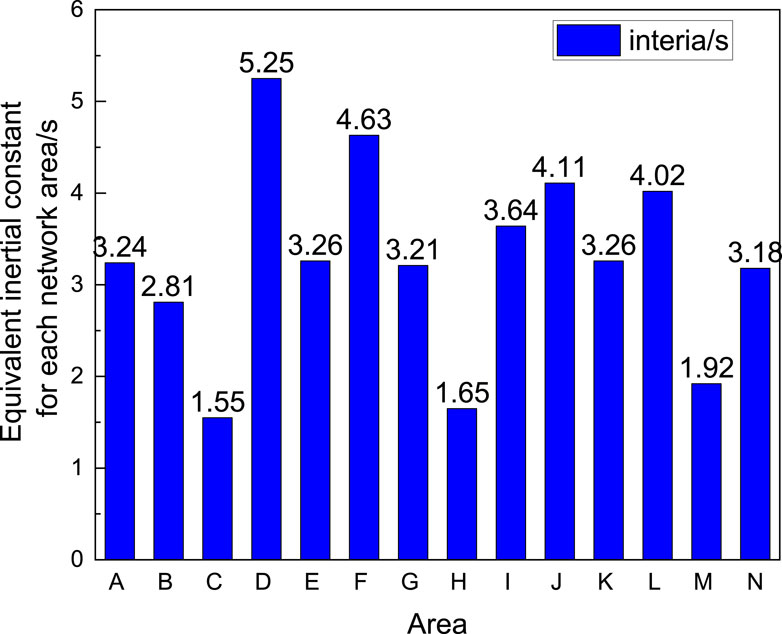
Figure 2. Statistical diagram of system inertia before new energy connection in each network area of a power grid in China.
Organize the new energy access capacity of various grid areas in a certain power grid in China, and compile the new energy access wind power capacity and photovoltaic capacity of each grid area in the power grid as shown in Figure 3.
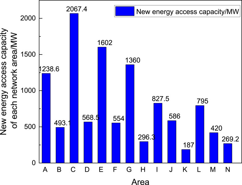
Figure 3. The statistical chart of total new energy access in various grid areas of a certain power grid in China.
Combining the new energy access capacities in various grid areas, organize and calculate the changes in system inertia levels before and after the large-scale integration of new energy in each grid area as shown in Table 1; Figure 4.
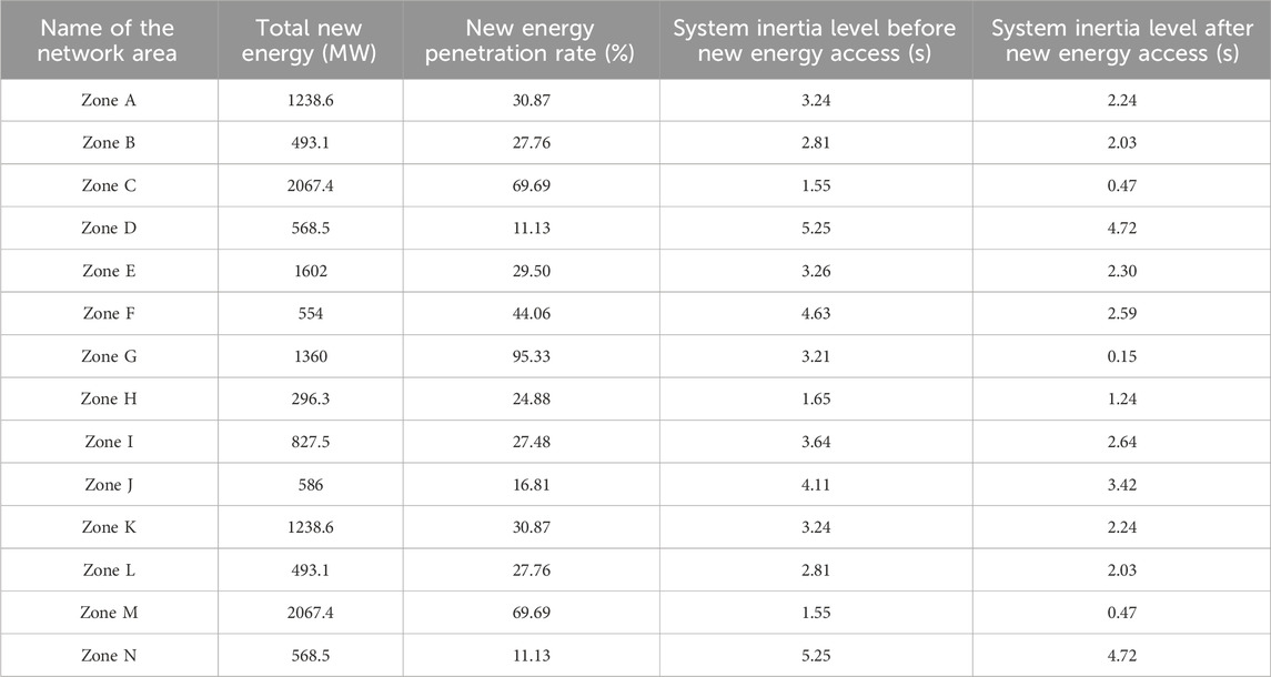
Table 1. Equivalent inertia statistics of various grid areas in a certain power grid in China under new energy access conditions.
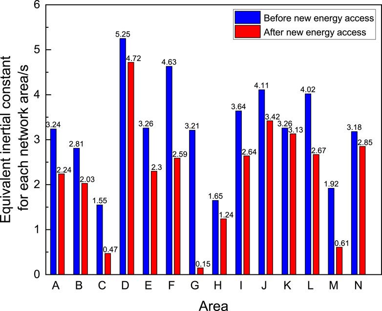
Figure 4. Statistical diagram of the system inertia constant before and after new energy access in each network area of a power grid in China.
Based on Figure 4; Table 1, it can be observed that the grid integration of new energy significantly affects the equivalent inertia level of a certain power system in China, leading to an exacerbation of the overall trend towards weaker system inertia. Before the integration of new energy, Area D had the highest inertia level, with an equivalent inertia constant of 5.25s, while Area C had the lowest inertia level at only 1.55s. After the integration of new energy, although Area D still maintains the highest inertia level, its equivalent inertia constant has decreased to 4.72s, while the inertia level of Area G has dropped to the lowest at 0.15s. The higher the penetration rate of new energy, the more significant the decrease in inertia constant for the grid areas. Among them, Area G, with the highest penetration rate of new energy at 95.33%, exhibits the most significant decrease in inertia and the lowest inertia level, while Area K has the lowest penetration rate of new energy at 4.45%, with its grid area inertia remaining relatively unchanged.
This indicates that due to the significant decrease in the system’s equivalent inertia level after the large-scale integration of new energy, the control of frequency fluctuations during the inertia response stage relies more on the relationship between unbalanced power and system kinetic energy. Since the inertia of the power system is mainly provided by synchronous generators before adopting virtual inertia control technology, the integration of new energy reduces the proportion of traditional synchronous machines, thereby reducing the system’s inertia level and posing a higher challenge to maintaining system frequency stability. To address this challenge, a comprehensive inertia assessment index and evaluation system will be established based on the equivalent inertia levels of various grid areas in the certain power grid of China, to quantitatively analyze the impact of new energy integration on grid stability and propose corresponding control strategies to ensure the safe and stable operation of the power system.
Incorporating the assessment system outlined in Section 1.2, an analysis of the equivalent inertia levels across various regions of the power grid in China was conducted, and a distribution map of inertia levels was generated as shown in Figure 5. Based on the inertia evaluation criteria, regions with equivalent inertia less than 2s, between 2s and 4s, and greater than 4s were marked in red, orange, and green, respectively. Among these regions, C, G, H, and M exhibit relatively low inertia levels. The low inertia in regions C and G can be attributed to their excessively high penetration rates of new energy, at 69.69% and 95.33%, respectively. The insufficient rotational inertia provided by synchronous generators within region H contributes to its low inertia level, with an equivalent inertia constant of 1.65s before the integration of new energy, indicating a severe inadequacy according to the evaluation criteria. Similarly, the low inertia level in region M is due to inadequate rotational inertia provided by synchronous generators and a high penetration rate of new energy. Prior to the integration of new energy, region M had an equivalent inertia constant of only 1.52s, indicating a severe inadequacy. Following the high proportion of new energy integration (with a penetration rate reaching 59.87%), the inertia level in region M further deteriorated, with the equivalent inertia constant plummeting to 0.61s due to the combined effect of both factors. The low inertia levels in these regions imply poor dynamic frequency response characteristics and higher risks of instability after disturbances, necessitating corresponding inertia compensation measures.
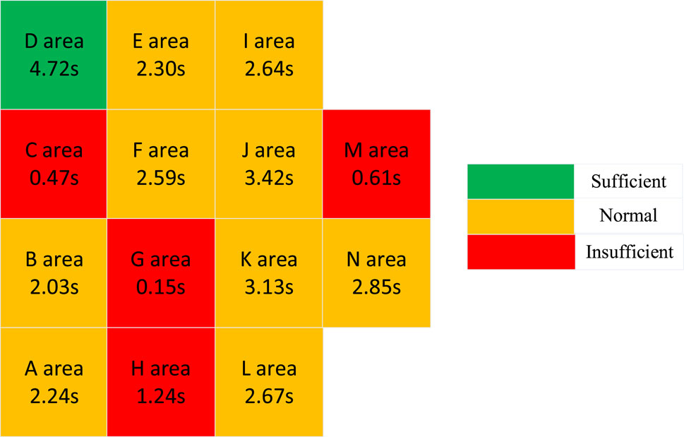
Figure 5. Inertia distribution heatmap of a power grid in China.
This section will utilize the node inertia calculation model proposed in Chapter 2, combined with the network parameters and generator dynamic parameters of a certain power grid in China, to calculate the inertia levels of nodes in the grid. Through this approach, we can identify weak points in inertia within the grid after the integration of renewable energy sources. To simplify the model, we will equivalently represent renewable energy units as traditional synchronous units of the same capacity but with lower inertia.
Based on the principles outlined in Section 2.2 and utilizing the BPA data of the specific Chinese power grid, the specific steps for calculating the inertia of nodes in the grid are as follows:
(1) Data preprocessing: The grid is simplified by conducting equivalence calculations based on power flow data, retaining only busbars and tie-lines of 10 kV and above, and eliminating isolated nodes. After simplification, the grid comprises 6,489 nodes, 7,171 branches, and 601 generator units, including 337 synchronous generators and 264 renewable energy units.
(2) Formation of the node admittance matrix for the Chinese power grid: Combining the network structure parameters from the BPA data forms the node admittance matrix for the entire grid. Calculation of the equivalent inertia levels of each grid area before the integration of renewable energy: The inertia constant Hi and corresponding capacity Si of traditional generator units in each grid area are calculated, and Eq. 2 is used to compute the equivalent inertia levels of each grid area before the integration of renewable energy.
(3) The load within each grid area is equivalently represented as grounding admittance, and the node admittance matrix generated from the first correction is modified. Additionally, generator nodes are augmented based on the modified node admittance matrix to obtain the system augmented admittance matrix.
(4) Based on the data from the augmented admittance matrix, the inertia levels of nodes in the entire Chinese power grid are calculated using Eq. 19.
Through the aforementioned steps, the calculated results of node inertia within grid areas are shown in Table 2 (taking the low inertia G grid area as an example, The first letter G in the bus name in the table represents the network area where the bus is located, the second and third letters represent the bus name, and the last two characters represent the generator node or transformer node).
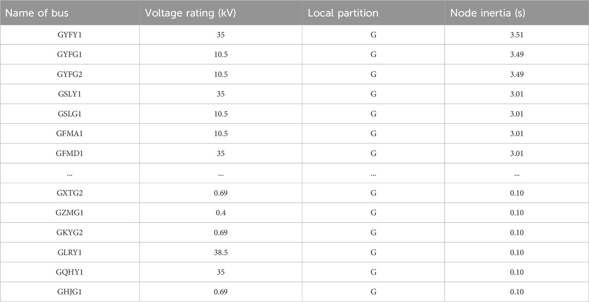
Table 2. Results of the inertia calculation of some nodes in region G.
According to Table 2, it is evident that there’s a significant uneven distribution of inertia within Zone G. The nodes with the highest inertia are concentrated among traditional synchronous generator units, particularly GYFG1, GYFG2 units, and their connected transformer nodes, with an equivalent inertia constant of approximately 3.5 s. This indicates that these nodes’ synchronous generators possess a high rotating mass, capable of providing strong inertia support to the grid, aiding in maintaining stability during disturbances. In contrast, the nodes with the lowest inertia in Zone G are primarily located among the renewable energy units and their connected transformer nodes, such as GHJG1, GKYG2, GLRY1, etc., with equivalent inertia constants of only 0.1 s. The low inertia of these nodes implies that in these areas, there’s insufficient rotating mass to counteract frequency fluctuations when the grid experiences frequency disturbances, thereby increasing the risk of instability in these regions.
The spatial distribution characteristics of renewable energy generation have a significant impact on the stability of the power grid. Due to the uneven distribution of wind and solar resources in different regions and the limitations imposed by natural geographic conditions on the grid connection locations of renewable energy generation units, this directly affects the distribution of inertia within different regions of the power grid. To reveal the spatial distribution patterns of inertia in each grid area of a certain power grid in China after the integration of renewable energy, the positions of the nodes with the maximum and minimum inertia in each grid area are compiled, as shown in Table 3:
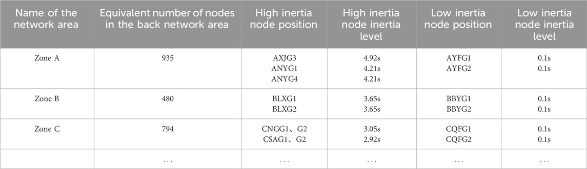
Table 3. Maximum and minimum inertia nodes in the Guangxi power grid.
From Table 3, it can be observed that areas where traditional large inertia synchronous generator units are connected, including the export-side busbars and those directly connected to them or with short electrical distances, exhibit higher levels of inertia. These regions typically house generators with substantial rotating masses, capable of providing robust inertia support to the grid, thereby aiding in maintaining system frequency stability. Conversely, areas where renewable energy generator units are connected display lower levels of inertia. This is attributed to the fact that renewable energy units, such as wind and solar, typically do not provide inertia response or offer significantly lower inertia response compared to traditional synchronous generator units. Consequently, regions near renewable energy units exhibit lower overall inertia levels, increasing the likelihood of system instability when subjected to disturbances.
In response to these areas of weakened inertia, corresponding compensatory measures need to be implemented in grid planning and operational management to enhance system stability. Potential compensation schemes include: installation of synchronous compensators or synchronous motors, which can provide additional inertia to help stabilize frequency fluctuations; deployment of energy storage systems such as flywheel energy storage or battery energy storage systems, capable of swiftly responding to grid frequency variations and supplying necessary power support; virtual inertia technologies utilizing power electronic devices like inverters to mimic inertia response and bolster grid disturbance resilience; optimization of dispatch strategies for renewable energy generation to mitigate system risks during periods of high renewable energy penetration; and strengthening interregional transmission line construction to enhance energy exchange capabilities between different regions, thereby improving overall grid robustness.
From Eqs 25, (26), it can be seen that under the conditions satisfying Eq. 26, the maximum inertia node in the system coincides with the system inertia center, and its inertia should be equal to the sum of the inertia of all synchronous generator units in the system. Given the fixed, discrete positions of the nodes in a multi-machine power system, it is difficult to verify the correctness of the above theory. In this section, a MATLAB two-area Simulink simulation model was established that satisfies the conditions of Eq. 26. The schematic diagram of the two-area system is shown below, and the parameters of the system are detailed in Supplementary Appendix SC:
Figure 6 depicts a schematic diagram of a 2-machine system. To validate the correctness of the derived theoretical result in Eq. 26, a model is constructed in Simulink. Disturbances are applied at various positions along the tie line, and the node inertia constants are calculated based on the disturbance magnitude and the rate of change of node frequencies. To minimize error, the average rate of change of frequencies from 0 to 0.05 s after the occurrence of disturbances is chosen. The distribution of node inertia constants for the two-machine system is shown in Figures 7, 8.
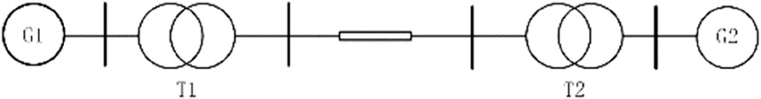
Figure 6. Diagram of simulink system with two regions.
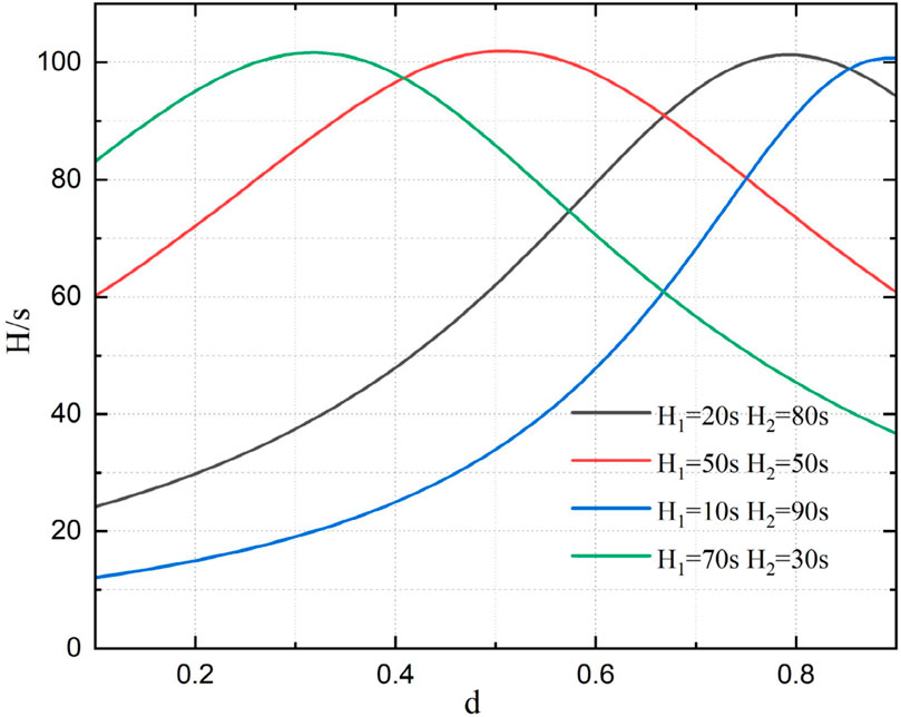
Figure 7. Diagram of node inertia level distribution with fixed total inertia.
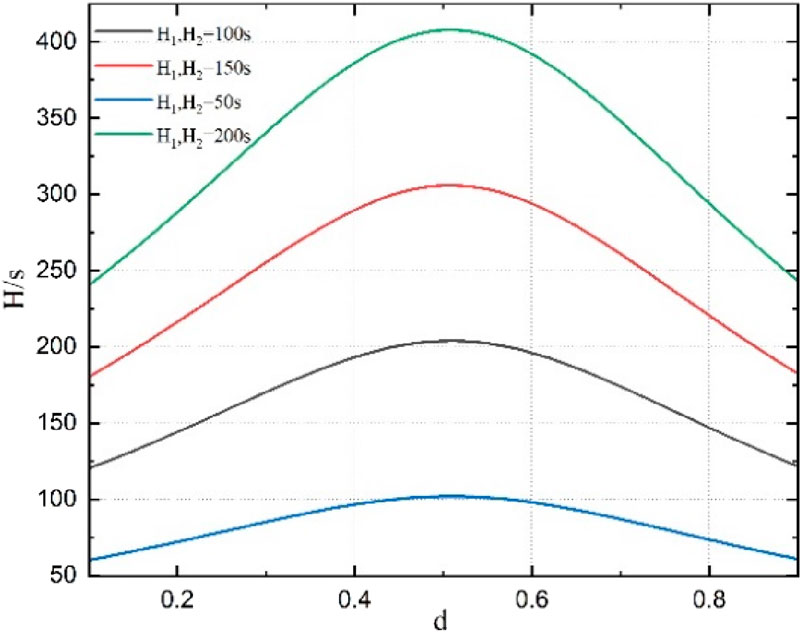
Figure 8. Diagram of node inertia constants with equal inertia of generators on both sides.
As shown in the above figure, the horizontal axis d represents the distance from node k to generator 1, expressed by the following equation:
In the equation,
Figures 7, 8 respectively illustrate the calculation of inertia constants at node k for different positions within the system, under scenarios where the inertia time constants H of generators on the left and right sides are different, the total inertia of the system varies, and the inertia constants of generators on both sides are equal. The summarized patterns are presented in Tables 4, 5.
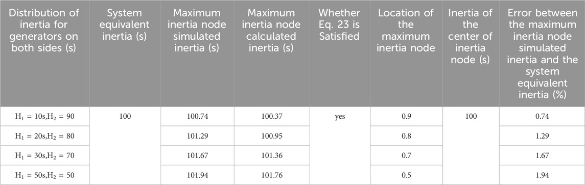
Table 4. Simulation distribution table of node inertia for a 2-machine system with constant total inertia.
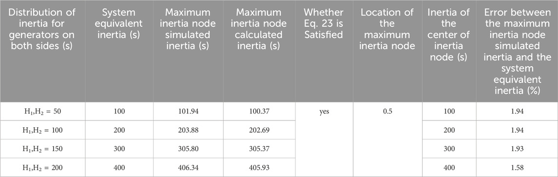
Table 5. Distribution table of node inertia for a 2-machine system with equal inertia of generators on both sides.
As listed in Table 4, when the total system inertia remains constant, and the inertia of generator units on both sides of the system varies, the position of the maximum inertia node and the inertia center changes. However, it always holds true that the maximum inertia node coincides with the inertia center, and its inertia value equals the system’s equivalent inertia. In Table 5, under the condition where the inertia of generator units on both sides is equal, the position of the maximum inertia node does not change with variations in the inertia of generators on both sides, and the inertia of the maximum inertia node equals the total system inertia. As indicated in the last column of both tables, there exists a discrepancy between the maximum inertia of nodes and the system’s equivalent inertia in the two simulation scenarios. This discrepancy arises due to two reasons: first, there are measurement errors in the power frequency values of node k during disturbance measurements in the simulation; second, the inertia response is instantaneous, and the rate of frequency change should be taken as the instantaneous value at the start of the disturbance. Since it is challenging to collect data at the instant of disturbance, the average rate of frequency change within 0–0.05s after the disturbance is chosen to reduce measurement errors. However, using the average value results in a smaller measured rate of frequency change compared to the actual rate, leading to measured data being greater than theoretical data. In summary, in Zone 2 of the system, when node k satisfies the condition in Eq. 26, the maximum inertia node coincides with the inertia center of the system, and its value theoretically equals the system’s equivalent inertia. The simulation experiment validates the correctness of the previous theoretical derivation.
The evaluation and selection of equivalent inertia assessment nodes in the power system involve detecting inertia equivalence at specific nodes within the system, substituting for system inertia. This is achieved by installing devices like PMUs at certain nodes to monitor power frequency changes, thereby calculating inertia to approximate the system’s inertia. This approach reduces evaluation complexity and the number of required monitoring devices, thus saving costs. Key to this process is selecting nodes for inertia assessment that closely match the system’s equivalent inertia level. From the above derivation, it is evident that when assessing system equivalent inertia using inertia calculation methods, the inertia assessment node corresponds to the node with the highest inertia in the system. Common methods for power system equivalent inertia assessment include the inertia centroid method and frequency centroid method. While these methods employ different assessment models, electrical distance calculation methods, and error reduction algorithms, they ultimately select nodes with higher inertia in the system. In this section, based on simulation analysis using the IEEE 39-node model, graph theory, and frequency centroid inertia assessment node positioning, the positions of inertia assessment nodes are compared with the location of the node with the highest inertia in the model, as detailed in Table 6.
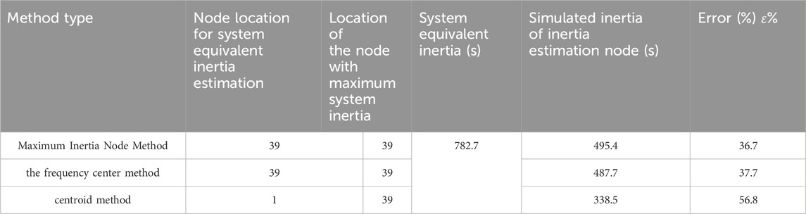
Table 6. Comparative analysis of three equivalent inertia estimation methods.
The location of the node with the maximum system inertia is calculated using Eq. 19, while the simulated inertia at the assessment node is determined by detecting power and frequency changes at the node in Simulink, combined with Eq. 3.
Based on Table 6, the system equivalent inertia assessment method based on frequency center selects the inertia detection node that coincides with the maximum inertia node, located at node 39. However, the inertia detection node chosen by the method based on the centroid does not overlap with the maximum inertia node, being located at nodes 1 and 39, respectively. This indicates that although the frequency center method proposes a different node selection approach, it actually selects the node with the maximum inertia in the system. In contrast, the centroid method’s inertia detection node and the maximum inertia node do not overlap. At least one node in the system is more suitable for the system equivalent inertia assessment than the selected measurement node, indicating some errors in this method for evaluating system equivalent inertia.
The inertia centroid method believes that the centroid should be located at a position with a smaller electrical distance from the system’s maximum inertia generating unit. The frequency center method suggests that the measurement node should be the one with the smallest initial frequency change rate after system disturbance. This conclusion is consistent with the previous Eqs 29, 30, which state that the maximum inertia node has the smallest frequency change rate after disturbance. This proves the correctness of the general rule that the system inertia detection node for equivalent inertia assessment should be the system’s maximum inertia node.
Due to the lack of rigorous mathematical derivation and unclear definition of electrical distance in methods like the centroid and frequency center methods, the maximum inertia node theory in this paper can serve as theoretical support for these methods. In the simulation scenario of this paper, there is a certain error between the inertia calculated at the maximum inertia node and the theoretical system value. This error is caused by the maximum inertia node in the multi-machine power system not satisfying the relationship in Eq. 26, where the system’s maximum inertia node and the inertia centroid do not overlap, and the inertia detected at the maximum inertia node should be less than the system’s equivalent inertia. However, using the maximum inertia node to assess the system’s equivalent inertia level can be considered a conservative evaluation method. When the inertia at the system’s maximum inertia node meets stability requirements, the real inertia level of the system should be greater than or equal to the system’s maximum inertia, indicating better stability. When using the maximum inertia node evaluation model to assess system inertia, the selection of the maximum inertia node requires knowledge of the inertia of each generator, network structure, and its parameters, and all node inertias must be calculated. This raises an issue: without knowing the inertia of each generator and the network structure and its parameters or having some missing information, it is impossible to calculate the inertia of each node or determine the inertia centroid using the aforementioned methods. This problem also exists in the inertia centroid and frequency center methods for assessing system inertia. In practice, to reduce the number of detection devices (for example, only one detection device is installed at the maximum inertia node in this paper) and lower costs, the number and location of installed devices must be predetermined before assessment. This method can be understood as a pre-determination of the number and location of detection devices. However, in actual operation, changes in the network structure and parameters may occur, causing the inertia centroid and its inertia to change. To completely solve this problem, detection devices could be installed at all bus nodes, but this would increase the evaluation cost.
The article addresses the issue of weak inertia caused by the integration of a high proportion of new energy into the grid. It conducts a comprehensive assessment of the inertia levels in various grid areas from both system and node perspectives. The research first establishes a model for evaluating equivalent inertia of grid areas and formulates inertia evaluation indicators. Secondly, it proposes a node inertia evaluation model based on grid structure parameters and synchronous power coefficients to assess the equivalent and node inertia levels of the grid, and explores the spatial distribution pattern of system inertia after the integration of new energy. Finally, it explores the correlation between equivalent inertia and node inertia, determines the nature of inertia evaluation nodes in equivalent inertia assessment research, and how to accurately identify them. The main conclusions drawn from the study are as follows:
(1) The trend of weak inertia in a certain Chinese grid due to the integration of a high proportion of new energy is evident, increasing the risk of instability after disturbances. Specifically, the inertia level is highest in zone D, while it is lowest in zone G, indicating a higher risk of instability in zone G when subjected to disturbances. According to the inertia evaluation indicators formulated in this study, zones C, G, H, and M have equivalent inertia levels of less than 2 s due to the high penetration rate of new energy, indicating a severe inadequacy. This suggests that additional inertia compensation measures need to be considered in these areas to enhance grid stability.
(2) Node inertia calculations are conducted for each grid area, with higher inertia levels near traditional large inertia synchronous units indicating better stability, while lower inertia levels near new energy units indicating poorer stability. The distribution of inertia in the entire grid follows a specific pattern: inertia levels are higher near the buses of traditional large inertia synchronous units and their directly connected buses with short electrical distances, while inertia levels are lower near the buses of new energy units and their connected buses. This distribution pattern suggests a gradual decrease in inertia levels from nodes of traditional large inertia units to nodes of weak inertia new energy units. The integration points of new energy units are weak links in system inertia and require additional inertia support to enhance grid stability.
(3) In inertia evaluation, the inertia evaluation node is the node with the maximum system inertia. When the maximum inertia node satisfies Eq. 26, the maximum inertia node coincides with the system inertia center, and at this time, the equivalent inertia of the maximum inertia node is the system equivalent inertia. Thus, there is an error in establishing the inertia evaluation node using the inertia centroid method. When conducting equivalent inertia evaluation of new energy power systems based on inertia calculation methods, it is only necessary to install PMU and other detection devices at the position of the maximum inertia node within the system to reduce installation costs.
The original contributions presented in the study are included in the article/Supplementary Material, further inquiries can be directed to the corresponding author.
JL: Writing–original draft, Writing–review and editing, Conceptualization, Formal Analysis, Investigation, Methodology, Project administration, Software, Supervision, Validation. PD: Data curation, Formal Analysis, Writing–original draft.
The author(s) declare that financial support was received for the research, authorship, and/or publication of this article. China Southern Power Grid supports related research in the paper. The funder was not involved in the study design, collection, analysis, interpretation of data, the writing of this article, or the decision to submit it for publication.
The authors declare that the research was conducted in the absence of any commercial or financial relationships that could be construed as a potential conflict of interest.
All claims expressed in this article are solely those of the authors and do not necessarily represent those of their affiliated organizations, or those of the publisher, the editors and the reviewers. Any product that may be evaluated in this article, or claim that may be made by its manufacturer, is not guaranteed or endorsed by the publisher.
The Supplementary Material for this article can be found online at: https://www.frontiersin.org/articles/10.3389/fenrg.2024.1418302/full#supplementary-material
Chen, G., Li, M., Xu, T., et al. (2017). Practice and challenges of power grid support for renewable energy development in China. Power Syst. Technol. 41 (10), 3095–3103. (in Chinese).
ENTSO-E (2020) The inertia challenge in Europe – present and long-term perspective. Brussels: ENTSO-E.
Jia, J., Yang, T., Yan, X., et al. (2023). Research progress on equivalent inertia evaluation of power electronic grid-connected equipment. Electr. Power Autom. Equip. 43 (09), 3–10. (in Chinese).
Li, D., Guo, T., Liu, Q., and Zhang, J. (2021). Evaluation of equivalent inertia of new energy power system considering photovoltaic power generation. Acta Energiae Solaris Sin. 42 (5), 174–179. (in Chinese).
Li, D., Zhang, J., Xu, Bo, et al. (2020). Evaluation of equivalent inertia of new energy power system considering frequency distribution characteristics. Power Syst. Technol. 44 (8), 2913–2921. (in Chinese).
Li, S., Jiang, Z., Cui, Yi, Kang, Y., Li, X., Li, H., et al. (2024). Enhanced dynamic state estimation of regional new energy power system under different abnormal scenarios. Int. J. Numer. Model. Electron. Netw. Devices Fields, 37, 32166-e3221. doi:10.1002/jnm.3216
Liu, F. (2021). Research on inertia assessment of new energy power system based on inertia distribution characteristics (China: North China Electric Power University). Master's Thesis.
Liu, F., Wang, F., et al. (2020). System partitioning inertia assessment method based on difference calculation method. Automation Electr. Power Syst. 44 (20), 46–53. (in Chinese).
Liu, F., Xu i, G., Liu, J., et al. (2021). Power system inertia distribution characteristics considering grid structure and parameters. Automation Electr. Power Syst. 45 (23), 60–67. (in Chinese).
Lu, Z., Jiang, J., Qiao, Y., et al. (2023). Review on generalized inertia analysis and optimization of new power system. Proc. Chin. Soc. Electr. Eng. 43 (05), 1754–1776. (in Chinese).
Milano, F., and Ortega, Á. (2017). Frequency divider. IEEE Trans. Power Syst. 32 (2), 1493–1501. doi:10.1109/pesgm.2017.8273830
State Administration for Market Regulation (2019) GB 38755-2019 Guidelines for the safety and stability of power systems. Beijing: China Standard Press. (in Chinese).
Sun, H., Wang, B., Li, W., et al. (2020). Study on inertia system of high proportion power electronic power system frequency response. Proc. Chin. Soc. Electr. Eng. 40 (16), 5179–5192. (in Chinese).
Tang, Q., Deng, C., Wang, Y., Guo, F. H., and Fan, S. (2024). Iterative observer-based resilient control for energy storage systems in microgrids under FDI attacks. IEEE Trans. Smart Grid, 1. early access. doi:10.1109/TSG.2024.3382125
Wen, Y., Yang, W., and Lin, X. (2020). Review and prospect of frequency stability analysis and control in low inertia power system. Electr. Power Autom. Equip. 40 (9), 211–222. (in Chinese).
Xiao, Y., Lin, X., and Wen, Y. (2020). Multi-dimensional evaluation of inertia level in DC and high-penetration new energy power grid. Electr. Power Constr. 41 (5), 19–27. (in Chinese).
Zeng, F. (2020). Identification method of power system inertia constant and its inertia temporal and spatial characteristics (China: South China University of Technology). Master's Thesis.
Zeng, F., and Zhang, J. (2020). Temporal and spatial characteristics of power system inertia and analysis methods. Proc. Chin. Soc. Electr. Eng. 40 (1), 50–58. (in Chinese).
Zhao, E., Han, Y., Zhou, S., et al. Review and prospect of inertia and damping simulation technology in microgrid. Proc. Chin. Soc. Electr. Eng., 2022, 42(04): 1413–1428. (in Chinese)
Zhou, X., Chen, S., Lu, Z., et al. (2018). Technical characteristics of China's new generation of power system in energy transition. Proc. Chin. Soc. Electr. Eng. 38 (7), 1893–1904. (in Chinese).
Keywords: partition equivalent inertia evaluation, node inertia evaluation, center of inertia, maximum inertia node, frequency monitoring node
Citation: Liu J and Di P (2024) New energy power system inertia weak position evaluation and frequency monitoring positioning. Front. Energy Res. 12:1418302. doi: 10.3389/fenrg.2024.1418302
Received: 16 April 2024; Accepted: 30 May 2024;
Published: 29 July 2024.
Edited by:
Yu Huang, Nanjing University of Posts and Telecommunications, ChinaReviewed by:
Chao Deng, Nanjing University of Posts and Telecommunications, ChinaCopyright © 2024 Liu and Di. This is an open-access article distributed under the terms of the Creative Commons Attribution License (CC BY). The use, distribution or reproduction in other forums is permitted, provided the original author(s) and the copyright owner(s) are credited and that the original publication in this journal is cited, in accordance with accepted academic practice. No use, distribution or reproduction is permitted which does not comply with these terms.
*Correspondence: Jiaji Liu, MjExMjMwMTA0MEBzdC5neHUuZWR1LmNu
Disclaimer: All claims expressed in this article are solely those of the authors and do not necessarily represent those of their affiliated organizations, or those of the publisher, the editors and the reviewers. Any product that may be evaluated in this article or claim that may be made by its manufacturer is not guaranteed or endorsed by the publisher.
Research integrity at Frontiers
Learn more about the work of our research integrity team to safeguard the quality of each article we publish.