A physical virtual multi-graph convolutional coordinated prediction method for spatio-temporal electricity loads integrating multi-dimensional information

Traditional load prediction methods are unable to effectively predict the loads according to the spatial topology of each electricity consumer in neighboring areas and the load dependency correlations. In order to further improve the load prediction accuracy of each consumer in the region, this paper proposes a short-term prediction method of electric load based on multi-graph convolutional network. First, the input data are selected with maximum information coefficient method by integrating multi-dimensional information such as load, weather, electricity price and date in the areas. Then, a gated convolutional network is used as a temporal convolutional layer to capture the temporal features of the loads. Moreover, a physical-virtual multi-graph convolutional network is constructed based on the spatial location of each consumer as well as load dependencies to capture the different evolutionary correlations of each spatial load. Comparative studies have validated the effectiveness of the proposed model in improving the prediction accuracy of power loads for each consumer.

1 Introduction

The global electricity demand is experiencing rapid growth, and the structure of urban distribution networks is becoming increasingly complex, which elevates the challenges associated with power grid scheduling and control (Hou et al., 2021). The ongoing expansion of hybrid renewable power systems has led to the integration of a substantial number of variable renewable energy sources, such as wind and solar, transforming the grid into an active distribution network. This transformation has concomitantly increased the volatility and uncertainty inherent to power systems (Cleary et al., 2015). Accurate load prediction is of paramount importance for enhancing the safety, stability, and efficient operation of the power grid (Celebi and Fuller, 2012). Furthermore, as power systems undergo reform, electricity sales companies and virtual power plants participating in the electricity market must accurately predict the electricity consumption of individual consumers (Aparicio et al., 2012).

The existing research on power load prediction can be broadly categorized into two primary methodological approaches: statistical models and machine learning techniques. The statistical modeling approach offers simplicity and expedient prediction capabilities. Prominent statistical methods include linear regression and exponential smoothing (Shi W. et al., 2023). Saber and Alam (2017) leveraged the autoregressive integrated moving average model to analyze the correlation between load demand and influential factors, and established a non-stationary stochastic prediction framework. However, such statistical techniques generally suffer from limitations in prediction accuracy and robustness. In contrast, machine learning methods possess adaptive and self-learning capabilities that have demonstrated improvements in load prediction precision. These advanced analytical techniques include support vector machines, extreme learning machines, long short-term memory (LSTM) networks, and convolutional neural networks (Li et al., 2020; Samadianfard et al., 2020; Zhang J. et al., 2021; Tang et al., 2021; Roy and Yeafi, 2022; Sun et al., 2023; Deng et al., 2024). Specifically, Li et al. (2020) proposed a power load decomposition and reconstruction prediction approach based on support vector machines. Furthermore, Roy and Yeafi (2022) and Sun et al. (2023) leveraged machine learning theory to establish residual self-attention encoding-decoding networks for electricity consumption and wind power prediction, effectively capturing the coupling relationships within the data. Additionally, Tang et al. (2021), Zhang J. et al. (2021) and Samadianfard et al. (2020) employed echo state networks, LSTM, and multi-layer perceptrons to predict wind direction, speed, and power generation. While the aforementioned methods utilize multi-dimensional information, such as load data and weather factors, to model the temporal correlations in load patterns, they have largely overlooked the potential spatial correlations in electricity consumption among multiple consumers. Neighboring consumers are affected by factors such as weather, electricity prices, and holidays, exhibiting similar electricity consumption behaviors and load profiles (Lin et al., 2021). Fully capturing and leveraging the spatial correlation information among these neighboring consumers has the potential to further improve the accuracy of load prediction. However, the non-Euclidean, interconnected graph structure of the consumer data limits the direct applicability of conventional neural network architectures, and thus necessitates specialized modeling approaches capable of learning from the complex spatial correlation of neighboring consumers.

Graph neural networks have attracted widespread attention because they can learn implicit representations of node data on graph structures and process non-Euclidean spatial data. Currently, graph neural networks have been successfully applied in fields such as transportation and load prediction. Yan et al. (2021) proposed a multi-time scale traffic prediction method based on graph convolutional networks, which treats each road sensor as a node to construct a spatio-temporal module and capture spatio-temporal correlations. Liao et al. (2023) established a three-dimensional Gaussian wake function that represents the relevant information of each wind turbine and used graph neural networks combined with attention mechanisms to predict the output power of non-uniform wind farms, reducing prediction errors. Shi P. et al. (2023) proposed a multi-user short-term power load spatio-temporal prediction method using multi-head attention and adaptive graph theory and compared it with various methods. Zhang L. et al. (2021) used K-means clustering to divide user groups, capture the intrinsic spatio-temporal correlation information of the data using local spatio-temporal graphs, and finally aggregate the calculation results of each part to predict the future spatio-temporal power demand sequence. Fahim et al. (2024) took a load of each charging station as a node, used an adaptive adjacency matrix to reflect the spatial relationship between stations, and proposed a multi-station charging demand prediction method for electric vehicle charging stations based on graph networks. Existing literature has shown that graph neural networks can explore potential relationships between loads and improve prediction accuracy. However, the above literature only considers the fixed spatial connection relationships of consumers and relies on a single graph representation, failing to reflect the various spatial correlations between electricity loads in the neighbors.

Multimodality neural networks have improved prediction accuracy, which has attracted the attention of researchers. Zheng et al. (2023) used virtual dynamic graph and physical road graph to extract heterogeneous, variable, and inherent spatial patterns of the road network. Liu et al. (2020) presented a physical-virtual collaboration graph neural network for passenger flow prediction. The network is a general model that can be directly applied to online pedestrian flow prediction. Xiu et al. (2024) adopted parallel convolutional networks and combines relational data within the metro network to predict ridership. In addition, the train timetable as feature input to the network, improving prediction accuracy. However, there is limited application of literature in load prediction. How to design a proper prediction network based on the characteristics of electricity demands is an important issue.

Multi-graph convolutional networks have been applied in literature for load prediction. Wei et al. (2023) presented a novel multi-graph neural networks for short-term electricity demand prediction, which is embedded with the directed static graph and directed dynamic graph. The results show that the network has a strong ability to capture periodic features. Yanmei et al. (2024) adopted dynamic load knowledge graph to extract the correlation between internal at-tributes and external influencing factors of various loads. Moreover, the attention mechanism enhances the learning ability of load feature representation. To capture complex non-linear correlations of loads, Wang et al. (2023) proposed spatial and temporal graph neural network for residential load prediction. The multiple dependence graphs consists of synchronization graph and causality graph, which can model linear and non-linear dependence. However, the exist research has not fully captured the in-dependence with multidimensional data, and electricity demand is associated with various complex and unknown factors. Therefore, predefined graphs cannot fully reflect load correlations. In addition, the coupling of spatio-temporal multidimensional information and the large amount of data make effective utilization to improve model performance another key issue.

This article proposes a multi-graph convolutional spatio-temporal collaborative prediction method for power load integrating multi-dimensional information. By constructing a multi-graph network, the spatial information of each consumer’s load is fully captured to improve prediction accuracy. First, based on historical load, weather, and electricity prices, the maximum information coefficient (MIC) is used to analyze the correlation of load sequence and to construct input data that integrates multi-dimensional information. Then, the network adopts a dilated convolution and gating mechanism to parallelly capture the practical information of temporal loads. Moreover, based on the actual location connection between consumers and the similarity of electricity loads, a physical, virtual multi-graph convolutional model is established to capture various interrelationships between loads in space. T the performance of the proposed model is tested on real electricity datasets and compared with other baseline models to verify its effectiveness.

The innovation of this paper is as the following:

• The gated casual convolution is adopted to accelerate the temporal convolution, which can capture correlation of time series information.

• We proposed a physical virtual multi-graph convolutional network to fully capture electricity load evolution patterns. The physical graph contains connection and distance data, which is based on realistic grid topology. The virtual graphs are built based on human domain knowledge.

Moreover, the main contribution of this paper is to use MIC to obtain the correlation of nonlinear influencing factors, which reduces input data redundancy. Specifically, this method filters out irrelevant spatio-temporal data and selects high MIC values as input, reducing the interference of input on the prediction results.

2 Spatio-temporal network of electricity loads

2.1 Spatial and temporal load structure

Stable electricity promotes the development of social production, and electricity is transmitted through power grid lines. The power consumption from different spatial locations is ultimately integrated into the power load of different grid nodes.As shown in Figure 1, different nodes in the grid topology correspond to electricity demand generated in different actual geographic areas. The load in an area corresponding to a grid node is regarded as the information of the nodes in the graph G, and the connection between grid nodes is regarded as the edges between the nodes in the graph G. We use the graph G(V, E, A) to describe the spatial load information, where V is a node, E is an edge, and A is an adjacency matrix, representing the connection between nodes. Each node in the graph G generates data with a total number of features F in a time interval. As shown in Figure 1, each time slice is a spatial graph that records the feature information of all nodes in the time interval.

Figure 1

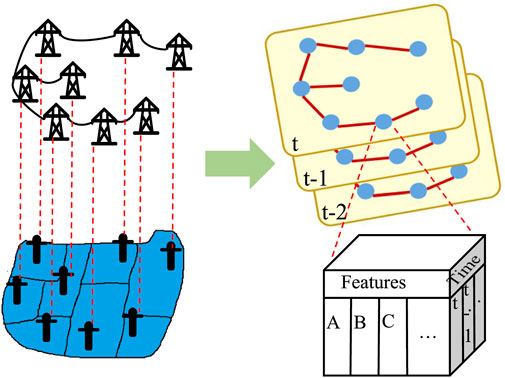
Figure 1. Spatial and temporal load structure diagram.

2.2 Definition of parameters and sets for electricity load prediction

Let the electricity load generated by each node in the graph in a future time period be the forecast data. Let $x_t^{f,i}$ be the features f generated by node i in the time interval t, then ${\mathit{X}}^c=({\mathit{x}}_1^f,\dots ,{\mathit{x}}_{\tau }^f)$ be the features f generated by all nodes in time period τ, and χ = (X₁, …, X_τ) be all features generated by all nodes in time period τ. It is assumed that the load $y_t^i=x_t^{f,i}$ generated by a node i at a certain time t, that is, all the characteristics χ including the load generated by all nodes within a certain time period are known. Then, the electricity load $\widehat{\mathit{Y}}=({\widehat{\mathit{y}}}^1,\dots ,{\widehat{\mathit{y}}}^N)$ for a certain time period in the future is predicted where ${\widehat{y}}^i$ is the electricity load during a certain time period of the node.

2.3 Maximum information coefficient

The main factors influencing load prediction are historical loads, weather conditions, time, and electricity prices (Quilumba et al., 2014; Sun et al., 2022). Table 1 summarizes the load influencing factors. Although applying influencing factors directly to neural networks as input data can also predict loads, excessive data increases computational complexity and speed. Using proper methods to select input data can improve prediction accuracy and accelerate computational speed. Therefore, this paper applies the maximum information coefficient theory for feature extraction.

Table 1

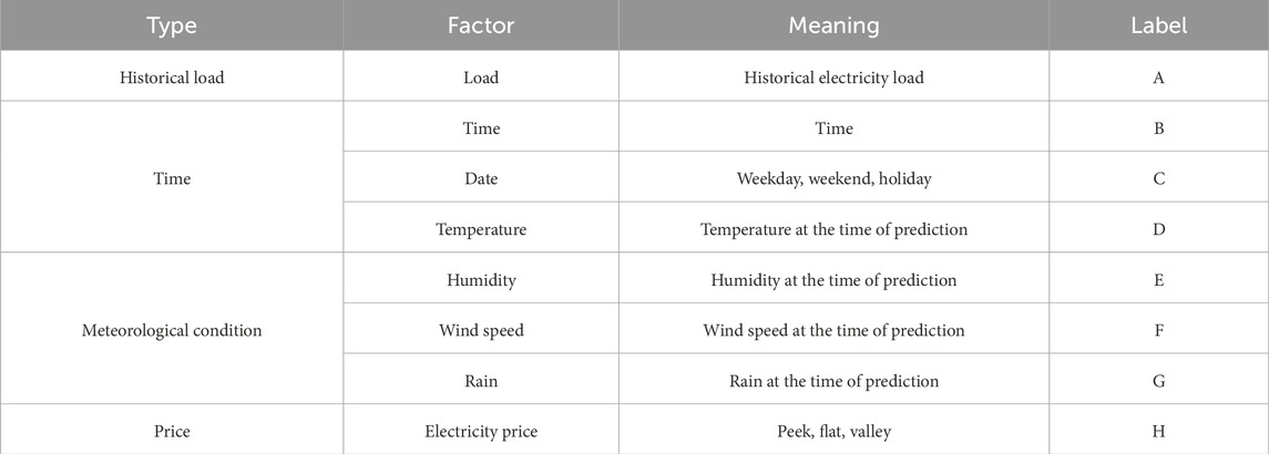
Table 1. Influencing factors of electric load.

The maximum information coefficient was proposed by Reshef based on mutual information theory (Reshef et al., 2011). MIC can analyze the linear and nonlinear correlation between two variables and screen parameters that affect load. The mutual information between sequences X_a and Y_a can be expressed as Eq. 1.

$I_{\text{m}}\left(X_{\text{a}},Y_{\text{a}}\right)={\displaystyle \sum _{x_{\text{a}}\in X_{\text{a}}}}{\displaystyle \sum _{y_{\text{a}}\in Y_{\text{a}}}}p\left(x_{\text{a}},y_{\text{a}}\right){\log }_2\frac{p\left(x_{\text{a}},y_{\text{a}}\right)}{p\left(x_{\text{a}}\right)p\left(y_{\text{a}}\right)}(1)$

where I_m(X_a, Y_a) represents mutual information, and p(⋅) is the probability density function, x_a ∈ X_a and y_a ∈ Y_a.

Let D_a = {(x_a,i, y_a,i), i = 1, …, n} be the set of binary data, and divide the value domains of X_a and Y_a into segments p_a and q_a in grid G_a. Define the maximum mutual information of D_a in grid G_a to be I_mi that is calculated using the Eq. 2.

$I_{\text{mi}}\left(D_{\text{a}},p_{\text{a}},q_{\text{a}}\right)=\max I_{\text{m}}\left(D_a\mid G_a\right)(2)$

where D_a∣G_a represents the data D_a divided by grid G_a.

Therefore, the maximum information coefficient is formulated as Eq. 3.

$I_{\text{mic}}\left(X_{\text{a}},Y_{\text{a}}\right)=\underset{p_{\text{a}}{q}_{\text{a}}<B\left(n\right)}{\max }\frac{I_{\text{mi}}\left(D_a,p_{\text{a}},q_{\text{a}}\right)}{{\log }_2\left(\min \left(p_{\text{a}},q_{\text{a}}\right)\right)}(3)$

where B_n is the limit on the number of grid divisions, generally B_n = n^0.6 (Reshef et al., 2011).

3 Spatio-temporal multi-graph prediction network

The spatio-temporal power prediction model mainly comprises a data embedding layer, a spatio-temporal prediction layer, and an output layer. The spatio-temporal prediction layer contains a temporal convolution module and a spatial multi-graph convolution module to capture the spatio-temporal correlation features of the data and the spatio-temporal dependencies of the data.

3.1 Data embedding layer

The data embedding layer consists of a convolutional network that transforms the input feature volume into high-dimensional data suitable for the spatio-temporal prediction layer. A standard convolutional network consists of three parts: convolutional, pooling, and fully connected layers, where the convolution is defined by Eq. 4

${\mathit{y}}_{\text{c}}=f\left({\mathit{x}}_{\text{in}}^{*}{\mathit{\omega }}_{\text{c}}+{\mathit{b}}_{\text{c}}\right)(4)$

where x_in is the input to the convolutional layer; ω_c is the convolutional kernel, i.e., the weight parameter; b_c is the bias value; f(⋅) is the convolution operation; is the activation function; y_c is the output value. In this paper, linear convolution is used to linearly transform the input data into high dimensional data by convolution operation, i.e., no activation function is used.

3.2 Spatio-temporal prediction layer

Mining the dependencies of loads in the time dimension can help improve prediction accuracy, and choosing an appropriate network structure is crucial. Recurrent neural networks have the structure of loops that accept data from themselves and other neurons and are particularly suitable for processing time-series data. However, deeper networks take a long time to compute results, and they are prone to gradient explosion and vanishing problems. In this paper, we choose convolutional neural networks with strong robustness and faster computation to capture the mutual characteristics of data in time.

3.2.1 Causal convolutional networks

Causal convolution is a special convolutional neural network that utilizes only past data in its computation. Its expansion factor can be controlled to quickly increase the receptive field, thus capturing load data for a longer period. As shown in Figure 2, causal convolution does not rely on data from future moments for computation compared to ordinary convolutional networks. In addition, stacking more layers of the null convolution can result in an exponential increase in the receptive field, covering more input data and speeding up the computation. The causal convolution can be expressed by Eq. 5 (Wu et al., 2019).

$\mathit{m}{\left(t\right)}^{*}{\mathit{x}}_{\text{d}}={\displaystyle \sum _{s=0}^{K-1}}\mathit{m}\left(s\right){\mathit{x}}_{\text{d}}\left(t-q_{\text{d}}s\right)(5)$

where m is the convolution kernel of the null convolution; s is the serial number of the convolution kernel; K is the size of the convolution kernel; x_d ∈ R^T is the input sequence; t is the moment; q_d is the dilation factor, i.e., the interval between two factors.

Figure 2

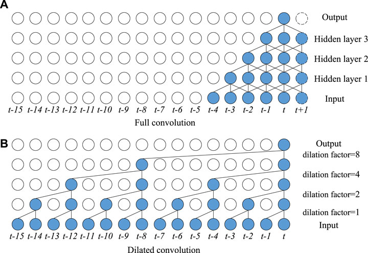
Figure 2. Convolutional network: (A)Full convolution, (B)Dilated convolution.

3.2.2 Gated mechanisms

Gating methods can selectively control the rate of data accumulation to avoid memory saturation. Combining the gating mechanism with a casual convolutional network can capture the complex relationship between loads in the temporal dimension, which has a significant advantage in processing sequential data. The output of the gating operation can be expressed as Eq. 6.

${\mathit{h}}_{\text{g}}=g_{\text{h}}\left({\mathit{\omega }}_{\text{h}}^{*}{\mathit{x}}_{\text{g}}\right)\odot g_{\text{s}}\left({\mathit{\omega }}_{\text{s}}^{*}{\mathit{x}}_{\text{g}}\right)(6)$

where x_g is the input data; ω_h and ω_s are the learnable model parameters; g_h(⋅) is the hyperbolic tangent function; g_s(⋅) is the Sigmoid function; ⊙ is the operator for multiplying elements; h_g is the output value. The temporal convolution module mined the features and correlations between power loads of the time series using gated null convolution network and fed the processed data into the spatial multi-graph convolution module.

3.3 Spatial multi-graph convolution module

In order to exploit the dependencies between electric loads in space, this section proposes a representation and calculation method of spatial loads based on spectral graph theory. Then, a physical-virtual multi-graph convolutional network based on the spatial location of loads and load similarity is built to represent the different dependencies of loads in the spatial dimension.

3.3.1 Spectral convolution

The graph load data is non-Euclidean space data, and each load node has a different connection relationship with other nodes. Moreover, the convolutional network is based on the translation invariant operation of the data, which cannot be directly applied to the non-Euclidean space. Bruna et al. (2014) defined graph convolution operation in spectral space based on graph theory and expressed the graph structure as a mathematical form. As a result, the non-Euclidean space data is transformed into Euclidean data for convolution operation.

In spectral theory, graph information can be represented by a Laplace matrix L. The equation is L = D − A and the standard form is $\mathit{L}={\mathit{I}}_{\mathbb{N}}-{\mathit{D}}^{\frac{1}{2}}\mathit{A}{\mathit{D}}^{\frac{1}{2}}$ where A is the adjacency matrix, D is the degree matrix, and I_N is the identity matrix. Let α_i,j and d_i,j be the elements of A and D, and i and j be the number of rows and columns, then d_i,j = ∑_ja_i,j. Decompose L into eigenvalues, L = UΛU^T, where U is the eigenvector and Λ is the diagonal array of eigenvalues. The graph convolution operation relies on the Fourier transform, defining the Fourier transform of the information on the graph x as $\widehat{x}={\mathit{U}}^{T}x$ and $\widehat{x}$ as the value of x in the spectral domain. Accordingly, the Fourien inverse transform of x is $x=\mathit{U}\widehat{x}$. By the convolution theorem, the Fourier transform of the convolution of signals is equal to the product of their individual Fourier transforms (Shuman et al., 2013). Therefore, it is possible to multiply the Fourier transform of the information on the graph by the information in the spectral domain and then invert the transformation to obtain the convolution result on the graph, as shown in Eq. 7.

${x*}_{G}z=\mathit{U}\left(\left({\mathit{U}}^{T}x\right)\odot \left({\mathit{U}}^{T}y\right)\right)=\mathit{U}{\mathit{g}}_{\theta }{\mathit{U}}^{T}x(7)$

where x and z are the signals on the graph; *_G is the graph convolution; g_θ is the convolution kernel, and g_θ = U^Tz

The graph convolution operation can be realized based on Eq. 7. However, calculating the Laplace matrix is cumbersome when the graph size is large. Therefore, the Chebyshev graph convolution approximation is used to solve the convolution kernel to simplify the operation:

${x*}_{G}z=\mathit{U}{\mathit{g}}_{\theta }{\mathit{U}}^{T}x\approx {\displaystyle \sum _m^{M-1}}{\theta }_m{T}_m\left(\tilde{\mathit{L}}\right)x(8)$

where θ_m is the Chebyshev polynomial coefficients; $T_m(\tilde{\mathit{L}})$ is the Chebyshev polynomial, $T_m(\tilde{\mathit{L}})=2\tilde{\mathit{L}}{T}_{m-1}(\tilde{\mathit{L}})-T_{m-2}(\tilde{\mathit{L}})$ and $T_0(\tilde{\mathit{L}})=1$, $T_1(\tilde{\mathit{L}})=\tilde{\mathit{L}}$; $\tilde{\mathit{L}}=2\mathit{L}/{\lambda }_{\max }-{\mathit{I}}_N$; and m is the order of Chebyshev polynomial.

The information in the graph is updated by the order information of itself and its neighboring nodes M − 1, and the depth of the transmitted information can be adjusted by controlling the maximum order M. In the actual calculation, the value of $\mathit{L}={\mathit{I}}_{\text{N}}-{\mathit{D}}^{-\frac{1}{2}}\mathit{A}{\mathit{D}}^{-\frac{1}{2}}$ is dispersed, so it is generally replaced ${\widehat{\mathit{D}}}^{-\frac{1}{2}}\widehat{\mathit{A}}{\widehat{\mathit{D}}}^{-\frac{1}{2}}$, where $\widehat{\mathit{A}}=\mathit{A}+{\mathit{I}}_N$ and $\widehat{\mathit{D}}$ are the degree matrices of $\widehat{\mathit{A}}$ (Yan et al., 2021).

An example of graph convolution operation is shown in Figure 3. Figure 3A is form of convolution, and the right side shows the convolution on non-Euclidean space. Figure 3B shows the spectral convolutional operation. Given a 6-bus grid, the adjacency matrix A and degree matrix D are obtained based on the grid. Then, we can get ${\mathit{D}}^{-\frac{1}{2}}\mathit{A}{\mathit{D}}^{-\frac{1}{2}}$. Given the input data ${\mathit{x}}_t^c$ and convolution kernel g_θ1, the result of graph convolution ${\mathit{x}}_t^c{*}_G\mathit{z}$ can be obtained.

Figure 3

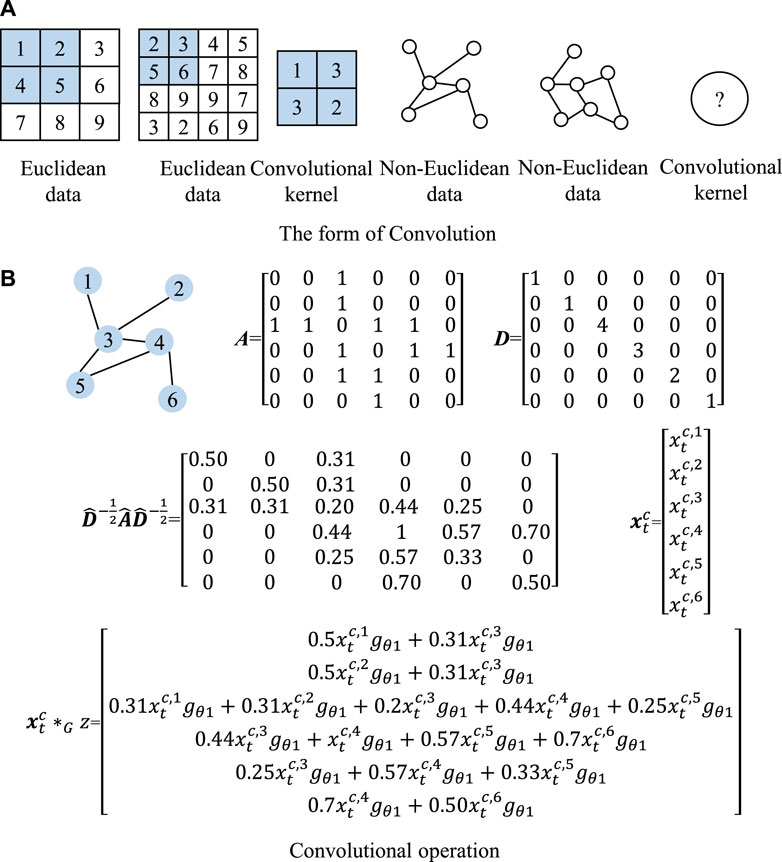
Figure 3. Graph convolution operation: (A)The form of convolution, (B)Convolutional operation.

The representation of the convolutional results on the network is further enhanced by the activation function ReLU:

${\mathit{h}}_{\text{f}}=g_{\text{r}}\left({\displaystyle \sum _m^{M-1}}{\theta }_m{T}_m\left(\tilde{\mathit{L}}\right)x\right)(9)$

where g_r is the activation function ReLU and h_f is the spatial convolution output.

3.3.2 Multi-graph construction

Different dependencies are implied between loads at different locations in space. The load relationship implied by the different interconnections and distances of electric loads in different regions is called neighborhood dependence, and the relationship implied by the different load similarities due to the different patterns of electricity use is called load correlation. In order to mine the proximity dependence and load correlation of electric loads at each location in space, a physical connectivity map, location distance map, and virtual correlation map are constructed.

1) Physical connection graph: The connection matrix is established based on the connection relationship between the lines where the power loads are located at each location, i.e., the interconnections of the nodes in the grid topology. The element of this matrix can be defined as Eq. 10.

$a_{i,j}^{\text{a}}=\left\{\begin{array}{c}1,\text{\hspace{0.17em}node\hspace{0.17em}}i\text{\hspace{0.17em}is\hspace{0.17em}connected\hspace{0.17em}to\hspace{0.17em}node\hspace{0.17em}}j\hfill \\ 0,\text{\hspace{0.17em}else\hspace{0.17em}}\hfill \end{array}\right.(10)$

2) Positional distance graph: A distance matrix is created based on the distance of the nodes where each power load is located A^d. The element of this matrix can be defined as Eq. 11.

$a_{i,j}^{\text{d}}=\left\{\begin{array}{cc}\exp \left(-\frac{d_{i,j}^2}{{\epsilon }_{\text{d}}^2}\right),\hfill & d_{i,j}\ge {\rho }_{\text{d}}\hfill \\ 0,\hfill & d_{i,j}<{\rho }_{\text{d}}\hfill \end{array}\right.(11)$

where $a_{i,j}^{\text{d}}$ is the element in A^d; d_i,j is the distance between node i and node j; ɛ_d is the matrix threshold parameter; ρ_d is the distance threshold parameter.

3) Virtual similarity graph: A similarity matrix is created based on the similarity between the electrical loads at each location A^s (Shi J. et al., 2023). The element of this matrix can be defined as Eq. 12, and the similarity between the load of node i and the load of node j can be calculated by Eq. 13.

$a_{i,j}^{\text{s}}=\mathrm{e}\mathrm{x}\mathrm{p}\left(-{\rho }_{\text{s}}{c}_{i,j}^{\text{d}}\right)(12)$

$c_{i,j}^{\text{d}}=\sqrt{{\displaystyle \sum _{t=1}^T}{\left(x_{t,i}^l-x_{t,j}^l\right)}^2}(13)$

where $a_{i,j}^{\text{s}}$ is the element in A^s; ρ_s is the parameter controlling the decay rate; $c_{i,j}^{\text{d}}$ is the similarity between the load of node i and the load of node j; $x_{t,i}^l$ and $x_{t,j}^l$ are the loads of node i and node j at time t.

The matrices A^a, A^d and A^s are used to obtain the corresponding L^a, L^d and L^s by bringing them into the standard computational form of the Laplace matrix, respectively. The Laplace matrices are brought into Eqs 8, 9 to obtain the convolution results of the loadings in each graph.

3.3.3 Multi-graph fusion

The graph fusion method is the key to graph neural networks, and a simple average summation of each graph will reduce the prediction performance. In this paper, we use the convolution results of each graph to be fused into a new graph by weighted summation to reflect the degree of influence of each graph in space. The weights of each graph are normalized using the Softmax function formulates as Eq. 14.

${\mathit{w}}_{\text{as}},{\mathit{w}}_{\text{ds}},{\mathit{w}}_{\text{ss}}=g_{\text{s\hspace{0.17em}o}}\left({\mathit{w}}_{\text{a}},{\mathit{w}}_{\text{d}},{\mathit{w}}_{\text{s}}\right)(14)$

where g_so is the Softmax function; w_a, w_d and w_s are the learnable weight parameters of the physical connectivity graph, positional distance graph and virtual association graph, respectively; w_as, w_ds and w_ss are the weights of the graphs after normalization, which indicate the influence degree of each graph in the new graph.

The weight parameters are multiplied with the results of the convolution of each graph and then summed, as shown in Eq. 15.

${\mathit{h}}_{\text{n\hspace{0.17em}e\hspace{0.17em}w}}={\mathit{w}}_{\text{a\hspace{0.17em}s}}\odot {\mathit{h}}_{\text{f}}^{\text{a}}+{\mathit{w}}_{\text{d\hspace{0.17em}s}}\odot {\mathit{h}}_{\text{f}}^{\text{d}}+{\mathit{w}}_{\text{s\hspace{0.17em}s}}\odot {\mathit{h}}_{\text{f}}^{\text{s}}(15)$

where h_new is the convolution result of the new graph; ${\mathit{h}}_{\text{f}}^{\text{a}}$, ${\mathit{h}}_{\text{f}}^{\text{d}}$ and ${\mathit{h}}_{\text{f}}^{\text{s}}$ are the convolution outputs of the physical connectivity graph, the positional distance graph and the virtual association graph, respectively.

The data features are extracted through the spatio-temporal convolution module, and the spatio-temporal convolution process is shown in Figure 4.

Figure 4

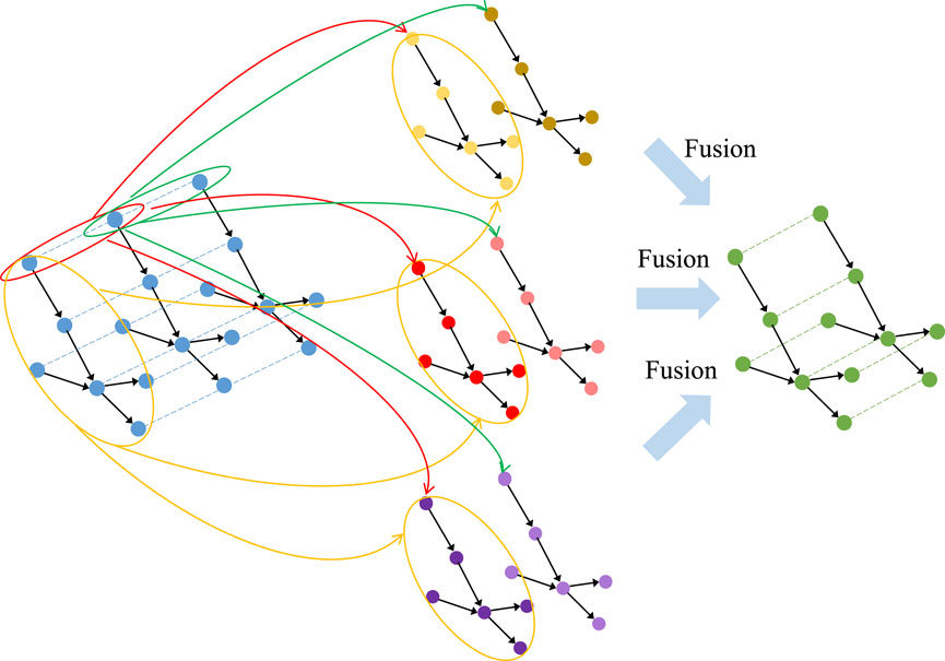
Figure 4. Spatio-temporal convolution.

3.4 Output layer

The output layer is connected to the spatio-temporal prediction layer, which converges and transforms the passed results into the desired dimensions. The use of linear convolution can effectively transform the data dimension, and the selection of an appropriate activation function can extract the nonlinear features of the data. Due to the large degree of nonlinearity and high dimensionality of the data, this paper adopts the ReLU activation function and linear convolution twice in series, i.e., the predicted power load value is finally obtained without losing too much information each time. The prediction step size of this network is adjustable, i.e., the load value can be obtained at one time for more than one moment.

3.5 Spatio-temporal multi-graph prediction network structure

Before inputting the data, the resulting data should be blank-filled, outliers removed, and corrected (Azeem et al., 2021). The features such as historical electric load power, weather, and date are filtered using maximum information coefficient analysis to select the most relevant features as input data into the prediction network. The structure of the spatio-temporal multi-graph prediction network is shown in Figure 5, and the corresponding multi-graph convolution algorithm is shown in Algorithm 1.

Figure 5

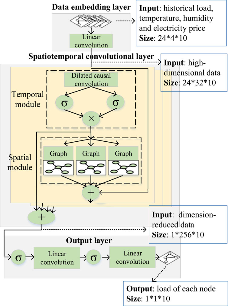
Figure 5. Spatio-temporal multi-graph prediction network structure.

The prediction network mainly comprises a data embedding layer, a spatio-temporal prediction layer, and an output layer. The spatio-temporal prediction layer consists of multiple temporal and spatial convolutional blocks stacked together, enabling the network to capture data correlations at different temporal levels. Different spatio-temporal convolutional blocks converge different levels of information to the output layer through skip connections. In addition, residual connections are utilized in the blocks to accelerate convergence and to address possible degradation of the deep network (He et al., 2016). The overall flowchart is shown in Figure 6.

Figure 6

Figure 6. The overall flowchart.

Algorithm 1.Spatio-temporal multi-graph prediction algorithm.

Input: Data set of ${\{{\mathit{X}}_i\}}_M$; the size of X_i is i*f*t; i is node, f is feature, and t is time.

Output: Multi-graph convolution model result $\widehat{\mathit{Y}}$;

1:   for each epoch do

2:   for each batch do

3:   Linear convolution: Conv(X_i) → X_start;

4:   Initial value 0 → X_res;

5:   for each spatio-temporal convolutional layer do

6    if first layer then

7:     X_start → X_in

8:    else

9:     Previous X_res is current X_in: X_res → X_in;

10:    end if

11:    Gated casual convolution: Conv(X_in) ⊙ Conv(X_in) → X_w;

12:    Skip connection: Y_skip + X_skip → Y_skip;

13:    Graph 1 convolution: G1conv(X_skip) → X_G1;

14:    Graph 2 convolution: G2conv(X_skip) → X_G2;

15:    Graph 3 convolution: G3conv(X_skip) → X_G3;

16:    Graphs fusion: X_G1 + X_G2 + X_G3 → X_res;

17:    Residual connection: X_res + Y_res → Y_res;

18:   end for

19:   Linear convolutions: Conv(Conv(Y_res)) → Y_out;

20:   Obtain MAE of network;

21:   Adjust hyperparameters;

22:  end for

23: end for

24:   Obtain result of $\widehat{\mathit{Y}}$.

3.6 Evaluation indicators

The performance of the prediction network is evaluated by applying Mean Absolute Error (MAE) I_MAE calculated by Eq. 16, Mean Absolute Percentage Error (MAPE) I_MAPE calculated by Eq. 17, Mean Squared Error (MSE) I_MSE calculated by Eq. 18, and Root Mean Squared Error (RMSE) I_RMSE calculated by Eq. 19. MAE is the difference between the predicted load and the actual load, which truly reflects the prediction error, and in this paper, we choose the Mean Absolute Error as the loss function of the network.

$I_{\text{M\hspace{0.17em}A\hspace{0.17em}E}}=\frac{1}{TM}{\displaystyle \sum _{t=1}^T}{\displaystyle \sum _{m=1}^M}\left|y_{t,m}-{\widehat{y}}_{t,m}\right|(16)$

$I_{\text{M\hspace{0.17em}A\hspace{0.17em}P\hspace{0.17em}E}}=\frac{1}{TM}{\displaystyle \sum _{t=1}^T}{\displaystyle \sum _{m=1}^M}\left|\frac{y_{t,m}-{\widehat{y}}_{t,m}}{y_{t,m}}\right|\times 100\%(17)$

$I_{\text{M\hspace{0.17em}S\hspace{0.17em}E}}=\frac{1}{TM}{\displaystyle \sum _{t=1}^T}{\displaystyle \sum _{m=1}^M}{\left(y_{t,m}-{\widehat{y}}_{t,m}\right)}^2(18)$

$I_{\text{R\hspace{0.17em}M\hspace{0.17em}S\hspace{0.17em}E}}=\sqrt{\frac{1}{TM}{\displaystyle \sum _{t=1}^T}{\displaystyle \sum _{m=1}^M}{\left(y_{t,m}-{\widehat{y}}_{t,m}\right)}^2}(19)$

where y_t,m and ${\widehat{y}}_{t,m}$ are the real and predicted values of load at time t node m respectively; m is the node number; and M is the total number of nodes.

4 Case study

4.1 Data set and parameters

In this paper, we use the 10 kV voltage level electric load dataset of a region in North China, including loads, weather conditions, date information and electricity prices, as shown in Table 2. All data have been desensitized and normalized to [0, 1]. The dataset contains a total of 10 bus data with a time range of 1 January 2020 to 1 June 2021, with a time interval of 60 min and a total of 24 points per day.

Table 2

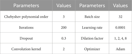
Table 2. Parameters of the model.

The predictive network model is implemented in Python software’s PyTorch learning library. In the debugging process of the network, considering the size of the data volume, the data set is taken as 70% as the training set, 20% as the validation set, and 10% as the test set. After several comparative analyses and comprehensive prediction performance, the model parameters are set as shown in Table 2. Among them, the Dropout means to make the neurons not work in a certain proportion, which can make the model generalization ability stronger. In addition, the model is a single-step prediction, i.e., all bus loads at the next moment are predicted using all bus data of the previous day. The framework of the model of this paper is illustrated in Figure 7.

Figure 7

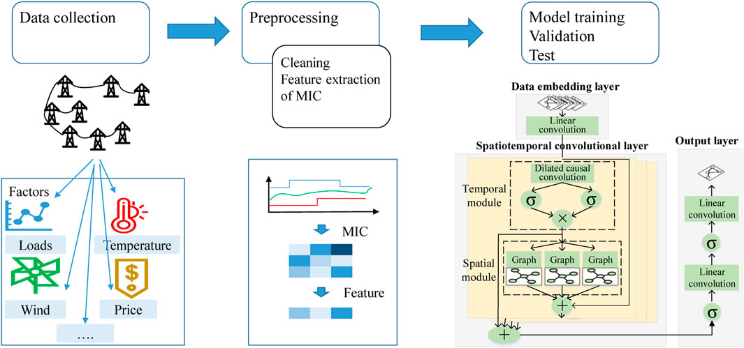
Figure 7. The framework of the model.

4.2 Feature selection results

The historical characteristics of Table 1 were analyzed by the maximum information coefficient analysis method to calculate the contribution of the influence of each characteristic quantity on the load, and the results are shown in Figure 8.

Figure 8

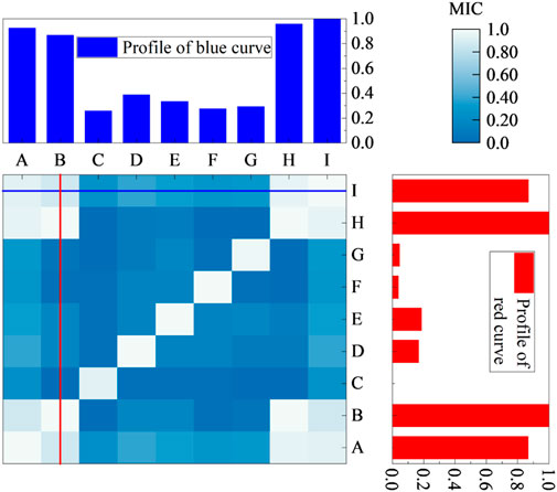
Figure 8. MIC of each feature.

The meanings of the letter labels in the graph are shown in Table 1, and label I is the predicted day load. It can be seen that the MIC of historical load, time and electricity price with forecast daily load is high, which represents a strong correlation. And the MIC between electricity price and time is 1, which represents a high correlation with cyclical changes in time and electricity price on a daily basis. Due to the higher MIC between electricity price and load, electricity price was chosen as one of the input features. The MIC for weather conditions is generally between 0.2 and 0.4, with temperature and humidity having a greater impact on load. Too much input data will reduce the computing speed of the model, in order to have better performance of the prediction network, this paper takes the threshold of MIC as 0.3. In summary, the input features are historical load, temperature, humidity and electricity price.

4.3 Analysis of forecast results

The neighbor matrices in the physical connection graph, location distance graph and virtual association graph of the prediction model are shown in Figure 9. It can be seen that since some of the nodes are not directly connected to each other, the elements of the connection matrix are 0. To control the sparsity of the graph, the distance matrix elements of the two nodes that are too close to each other are set to 0 to improve the speed of operation. The similarity matrix elements vary as the nodes have different power usage patterns. We adjust the parameters ρ_s to make the distribution of the adjacency matrix more uniform. Applying the proposed spatio-temporal multi-graph prediction model, the metrics for evaluating power load forecasts at 10 nodes are shown in Table 3.As can be seen from Table 3, the mean absolute error varies from node to node due to their different load characteristics, and the overall MAE is 0.0136. The node 4 has a smaller MAE and a larger MAPE due to its small load power and high degree of fluctuation. However, node 6 and node 7 have irregular daily power loads with high uncertainty, resulting in larger MAPE and MSE. Node 3, node 5, node 8 and node 9 have smooth and distinctly cyclical load variations and have higher predicted MAPE. Node 1 has a higher load MAE and MAPE than node 5, but low MSE and RMSE, which indicates a higher degree of deviation from the individual results of the predictive model at node 5. Overall, the multigraph convolutional model predicted a MAPE of 5.26%.

Figure 9

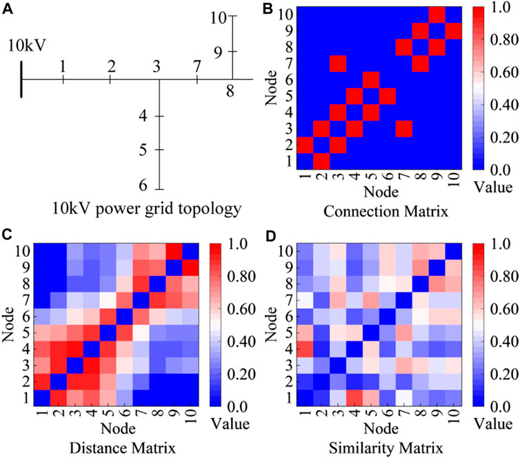
Figure 9. The adjacency matrices of the graphs: (A) 10 kV power grid topolpgy, (B) Convolution matrix, (C) Distance matrix, (D) Similarity matrix.

Table 3

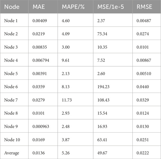
Table 3. Load prediction results of each node.

4.4 Model comparison

To further validate the performance of the spatio-temporal multi-graph prediction network, it is compared with the following four widely used prediction networks:

1) Historical Average (HA): this model takes the average of the most recent load data as the predicted value and is one of the most classical statistical methods;

2) Gated Recurrent Unit (GRU): this network is a type of recurrent neural network that employs a gating mechanism to filter out the information in the long term sequences, thus improving the prediction performance;

3) Convolutional Neural Network-Long Short-term Memory Network (CNN-LSTM): this network utilizes a convolutional neural network to extract valid information from the input data. Due to the ability of LSTM to handle longer time series, they are integrated into the CNN for prediction;

4) Spatio-Temporal Convolutional Network (STGCN): this network consists of gated linear units to extract temporal features, graph convolutional networks to extract spatial features, and multiple spatio-temporal blocks superimposed to form a prediction network (Yu et al., 2017).

The prediction results are shown in Table 4. It can be seen that the performance of the multi-graph convolutional prediction model proposed in this paper are satisfactory. Since HA relies on simple averaging of historical loads to obtain the results, it is unable to capture the nonlinear factors of power loads in the time series, and thus has the lowest prediction accuracy. The GRU, a neural network with memory function, captures the correlation features of loads in the time series, with a MAPE of 6.62%, which reduces by 1.44% compared with that of HA, and achieves a better result. CNN-LSTM utilizes the convolutional network to process the feature information of the input load, which further reduces the MAPE by 0.31%.STGCN, a classical graph neural network, predicts a MAE of 0.0152 and a MAPE of 5.63%, which outperforms the traditional neural networks and statistical models. This is due to the fact that graph convolutional networks can process non-Euclidean load information and capture the hidden information of spatial loads. Due to the use of physical-virtual multi-graph structure to mine the different evolutionary relationships of loads in space, the proposed method has a MAPE of 5.26%, which is the best performance. The predicted MAE and MAPE evaluation metrics for each comparison method at each node load are shown in Figure 10.

Table 4

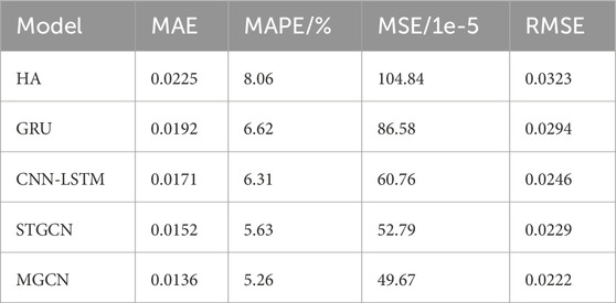
Table 4. Load forecasting results of different methods.

Figure 10

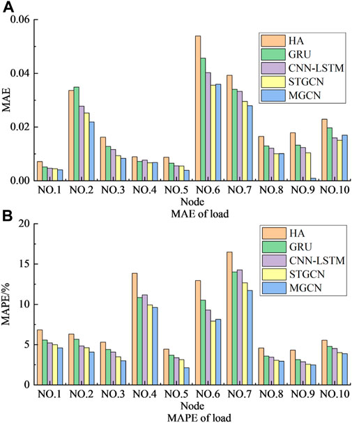
Figure 10. MAE and MAPE of each node: (A) MAE of load, (B) MAPE of load.

It can be seen that the MAE and MAPE of each method are different due to the different fluctuation patterns of electric loads at each node. HA is a classical statistical model with large prediction errors in predicting more volatile loads such as nodes 4, 6 and 7. While deep learning models such as GRU and CNN-LSTM have less difference in MAPE at each node. The prediction networks with graph structure such as STGCN and MGCN can learn the potential relationship of each node and can further reduce the prediction error of each load.

4.5 Ablation experiments

In order to analyze the contribution of each module in the proposed physical virtual multi-graph network structure, we design ablation experiments. We compare the proposed model with the following variants:

• MGCN: The model is the proposed network, which contains the multi-graph and temporal convolutional network simultaneously.

• PC-GCN: In this variant, we retain the physical connection graph and remove the other graphs.

• P-GCN: Similarly, the virtual similarity graph is removed, retaining the positional graph and the physical connection graph.

• VS-GCN: This variant adopts virtual similarity matrix as features of graph, without employing the physical connection and distance graph.

• TCN: Different with above variants that contain the graph network, the variant is constructed with only temporal convolutional network.

The performances of different variants is shown in Table 5.

In Table 5, TCN obtains the MAPE of 6.40, which is similar to the performance of GRU and CNN-LSTM. Due to the lack of graph modules, they can only capture temporal features of data. When there is a physical graph in the model, the error in load prediction decreases significantly. In addition, We can observe that the MAE of P-GCN is very close to that of the STGCN. This indicates that physical graphs can extract hidden patterns of loads in the spatial dimension. We further combine a virtual similarity graph with the convolutional network, which achieves superior performance. Notably, the proposed virtual graph based on human domain knowledge can fully explore the evolution patterns of electricity loads.

Table 5

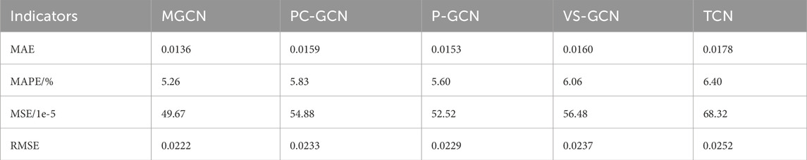
Table 5. Load prediction results of different modules.

5 Conclusion

In order to fully explore the correlation of various modes between the power loads of each node, this paper proposes a multi-graph convolutional spatio-temporal synergistic prediction method for power loads by fusing multi-dimensional information, and the theoretical analysis and the results of the arithmetic examples show that:

1) The maximum information coefficient method can effectively analyze load prediction influencing factors, select the most relevant features and reduce the redundancy of input information;

2) The non-Euclidean load information is processed by using spectral graph theory, and the constructed physical-virtual multi-graph convolutional network mines multiple spatial relationships between loads at each node, enriches the spatial characteristics of loads and improves the prediction accuracy;

3) Compared with statistical models, traditional neural networks and graph convolution models, the multi-graph spatio-temporal prediction network proposed in this paper has high prediction accuracy, which verifies the effectiveness of the method;

Although this paper has made some progress in constructing multi-graph convolution for spatio-temporal load prediction, the graph convolution network needs to be improved further: 1) The superior performance of the graph convolution network requires multiple rounds of manual hyperparameter tuning. More generalized and concise prediction networks can be considered for future adoption to improve the model’s quality. 2) The electricity demand periodically changes over a large period. For example, the electricity load during the New Year is usually similar. We can add modules to learn load characteristics if there is continuous electricity data for every year. 3) We will design more general prediction models to achieve robust performance with incomplete data.

Data availability statement

The original contributions presented in the study are included in the article/supplementary material, further inquiries can be directed to the corresponding author.

Author contributions

YJ: Supervision, Writing–original draft. WC: Conceptualization, Methodology, Software, Writing–original draft. XW: Software, Validation, Writing–original draft. YZ: Data curation, Writing–review and editing. JZ: Validation, Writing–review and editing. WM: Software, Writing–review and editing.

Funding

The authors declare that financial support was received for the research, authorship, and/or publication of this article. This work is supported by the Science and Technology Project of State Grid Shanxi Electric Power Company Limited (no. 5205E0220001).

Conflict of interest

Authors WC, XW, YJ, YZ, JZ, and WM were employed by State Grid Shanxi Electric Power Company Limited.

The authors declare that this study received funding from the Science and Technology Project of State Grid Shanxi Electric Power Company Limited. The funder had the following involvement in the study: conceptualization, data curation and formal analysis, visualization, writing the original draft and editing.

Publisher’s note

All claims expressed in this article are solely those of the authors and do not necessarily represent those of their affiliated organizations, or those of the publisher, the editors and the reviewers. Any product that may be evaluated in this article, or claim that may be made by its manufacturer, is not guaranteed or endorsed by the publisher.

References

Aparicio, N., MacGill, I., Abbad, J. R., and Beltran, H. (2012). Comparison of wind energy support policy and electricity market design in europe, the United States, and Australia. IEEE Trans. Sustain. Energy 3, 809–818. doi:10.1109/tste.2012.2208771

CrossRef Full Text | Google Scholar

Azeem, A., Ismail, I., Jameel, S. M., and Harindran, V. R. (2021). Electrical load forecasting models for different generation modalities: a review. IEEE Access 9, 142239–142263. doi:10.1109/access.2021.3120731

CrossRef Full Text | Google Scholar

Bruna, J., Zaremba, W., Szlam, A., and LeCun, Y. (2014). “Spectral networks and deep locally connected networks on graphs, 2nd int,” in Conf. on Learning Representations, ICLR 2014—Conference Track Proceedings, Banff, AB, Canada, April 14-16, 2014.

Google Scholar

Celebi, E., and Fuller, J. D. (2012). Time-of-use pricing in electricity markets under different market structures. IEEE Trans. Power Syst. 27, 1170–1181. doi:10.1109/tpwrs.2011.2180935

CrossRef Full Text | Google Scholar

Cleary, B., Duffy, A., Oconnor, A., Conlon, M., and Fthenakis, V. (2015). Assessing the economic benefits of compressed air energy storage for mitigating wind curtailment. IEEE Trans. Sustain. Energy 6, 1021–1028. doi:10.1109/tste.2014.2376698

CrossRef Full Text | Google Scholar

Deng, J., Wu, J., Zhang, S., Li, W., and Wang, Y.-G. (2024). Physical informed neural networks with soft and hard boundary constraints for solving advection-diffusion equations using fourier expansions. Comput. Math. Appl. 159, 60–75. doi:10.1016/j.camwa.2024.01.021

CrossRef Full Text | Google Scholar

Fahim, S. R., Atat, R., Kececi, C., Takiddin, A., Ismail, M., Davis, K. R., et al. (2024). “Forecasting ev charging demand: a graph convolutional neural network-based approach,” in 2024 4th International Conference on Smart Grid and Renewable Energy (SGRE), Doha, Qatar, 8-10 January 2024, 1–6.

CrossRef Full Text | Google Scholar

He, K., Zhang, X., Ren, S., and Sun, J. (2016). “Deep residual learning for image recognition,” in Proceedings of the IEEE conference on computer vision and pattern recognition, Seattle, WA, USA, June 14-19, 2020, 770–778.

CrossRef Full Text | Google Scholar

Hou, H., Chen, Y., Liu, P., Xie, C., Huang, L., Zhang, R., et al. (2021). Multisource energy storage system optimal dispatch among electricity hydrogen and heat networks from the energy storage operator prospect. IEEE Trans. Industry Appl. 58, 2825–2835. doi:10.1109/tia.2021.3128499

CrossRef Full Text | Google Scholar

Li, G., Li, Y., and Roozitalab, F. (2020). Midterm load forecasting: a multistep approach based on phase space reconstruction and support vector machine. IEEE Syst. J. 14, 4967–4977. doi:10.1109/jsyst.2019.2962971

CrossRef Full Text | Google Scholar

Liao, W., Wang, S., Bak-Jensen, B., Pillai, J. R., Yang, Z., and Liu, K. (2023). Ultra-short-term interval prediction of wind power based on graph neural network and improved bootstrap technique. J. Mod. Power Syst. Clean Energy 11, 1100–1114. doi:10.35833/mpce.2022.000632

CrossRef Full Text | Google Scholar

Lin, W., Wu, D., and Boulet, B. (2021). Spatial-temporal residential short-term load forecasting via graph neural networks. IEEE Trans. Smart Grid 12, 5373–5384. doi:10.1109/tsg.2021.3093515

CrossRef Full Text | Google Scholar

Liu, L., Chen, J., Wu, H., Zhen, J., Li, G., and Lin, L. (2020). Physical-virtual collaboration modeling for intra-and inter-station metro ridership prediction. IEEE Trans. Intelligent Transp. Syst. 23, 3377–3391. doi:10.1109/tits.2020.3036057

CrossRef Full Text | Google Scholar

Quilumba, F. L., Lee, W.-J., Huang, H., Wang, D. Y., and Szabados, R. L. (2014). Using smart meter data to improve the accuracy of intraday load forecasting considering customer behavior similarities. IEEE Trans. smart grid 6, 911–918. doi:10.1109/tsg.2014.2364233

CrossRef Full Text | Google Scholar

Reshef, D. N., Reshef, Y. A., Finucane, H. K., Grossman, S. R., McVean, G., Turnbaugh, P. J., et al. (2011). Detecting novel associations in large data sets. science 334, 1518–1524. doi:10.1126/science.1205438

PubMed Abstract | CrossRef Full Text | Google Scholar

Roy, A. D., and Yeafi, A. (2022). “Implementation of encoder-decoder based long short-term memory network for short-term electrical load forecasting,” in 2022 4th International Conference on Sustainable Technologies for Industry 4.0 (STI) (IEEE), Dhaka, Bangladesh, Dec. 17 2022 to Dec. 18 2022, 1–6.

CrossRef Full Text | Google Scholar

Saber, A. Y., and Alam, A. R. (2017). “Short term load forecasting using multiple linear regression for big data,” in 2017 IEEE symposium series on computational intelligence (SSCI) (IEEE), Honolulu, Hawaii, USA, 27 November - 1 December 2017, 1–6.

CrossRef Full Text | Google Scholar

Samadianfard, S., Hashemi, S., Kargar, K., Izadyar, M., Mostafaeipour, A., Mosavi, A., et al. (2020). Wind speed prediction using a hybrid model of the multi-layer perceptron and whale optimization algorithm. Energy Rep. 6, 1147–1159. doi:10.1016/j.egyr.2020.05.001

CrossRef Full Text | Google Scholar

Shi, J., Zhang, W., Bao, Y., Gao, D. W., and Wang, Z. (2023a). Load forecasting of electric vehicle charging stations: attention based spatiotemporal multi-graph convolutional networks. IEEE Trans. Smart Grid 15, 3016–3027. doi:10.1109/tsg.2023.3321116

CrossRef Full Text | Google Scholar

Shi, P., Geng, L., Zhang, M., Xu, D., and Li, H. (2023b). “A short-term regional net load prediction method based on parallel fragment attention-bi-lstm,” in 2023 IEEE 6th International Conference on Automation, Electronics and Electrical Engineering (AUTEEE) (IEEE), Shenyang, China, December 15, 2023 - December 17, 2023, 624–629.

CrossRef Full Text | Google Scholar

Shi, W., Li, Y., Dong, S., Lu, X., Ye, H., and Hu, B. (2023c). “Short term load forecasting for holidays based on exponential smoothing of correlative correction,” in 2023 International Conference on Power System Technology (PowerCon) (IEEE), Kuala Lumpur, Malaysia, 12-14 September 2022, 1–4.

CrossRef Full Text | Google Scholar

Shuman, D. I., Narang, S. K., Frossard, P., Ortega, A., and Vandergheynst, P. (2013). The emerging field of signal processing on graphs: extending high-dimensional data analysis to networks and other irregular domains. IEEE signal Process. Mag. 30, 83–98. doi:10.1109/msp.2012.2235192

CrossRef Full Text | Google Scholar

Sun, S., Du, Z., Jin, K., Li, H., and Wang, S. (2023). Spatiotemporal wind power forecasting approach based on multi-factor extraction method and an indirect strategy. Appl. Energy 350, 121749. doi:10.1016/j.apenergy.2023.121749

CrossRef Full Text | Google Scholar

Sun, S., Li, M., Wang, S., and Zhang, C. (2022). Multi-step ahead tourism demand forecasting: the perspective of the learning using privileged information paradigm. Expert Syst. Appl. 210, 118502. doi:10.1016/j.eswa.2022.118502

CrossRef Full Text | Google Scholar

Tang, Z., Zhao, G., and Ouyang, T. (2021). Two-phase deep learning model for short-term wind direction forecasting. Renew. Energy 173, 1005–1016. doi:10.1016/j.renene.2021.04.041

CrossRef Full Text | Google Scholar

Wang, Y., Rui, L., Ma, J., and jin, Q. (2023). A short-term residential load forecasting scheme based on the multiple correlation-temporal graph neural networks. Appl. Soft Comput. 146, 110629. doi:10.1016/j.asoc.2023.110629

CrossRef Full Text | Google Scholar

Wei, C., Pi, D., Ping, M., and Zhang, H. (2023). Short-term load forecasting using spatial-temporal embedding graph neural network. Electr. Power Syst. Res. 225, 109873. doi:10.1016/j.epsr.2023.109873

CrossRef Full Text | Google Scholar

Wu, Z., Pan, S., Long, G., Jiang, J., and Zhang, C. (2019). Graph wavenet for deep spatial-temporal graph modeling. arXiv preprint arXiv:1906.00121.

Google Scholar

Xiu, C., Zhan, S., Pan, J., Peng, Q., Lin, Z., and Wong, S. (2024). Correlation-based feature selection and parallel spatiotemporal networks for efficient passenger flow forecasting in metro systems. Transp. A Transp. Sci., 1–37. doi:10.1080/23249935.2024.2335244

CrossRef Full Text | Google Scholar

Yan, B., Wang, G., Yu, J., Jin, X., and Zhang, H. (2021). Spatial-temporal Chebyshev graph neural network for traffic flow prediction in iot-based its. IEEE Internet Things J. 9, 9266–9279. doi:10.1109/jiot.2021.3105446

CrossRef Full Text | Google Scholar

Yanmei, J., Mingsheng, L., Yangyang, L., Yaping, L., Jingyun, Z., Yifeng, L., et al. (2024). Enhanced neighborhood node graph neural networks for load forecasting in smart grid. Int. J. Mach. Learn. Cybern. 15, 129–148. doi:10.1007/s13042-023-01796-8

CrossRef Full Text | Google Scholar

Yu, B., Yin, H., and Zhu, Z. (2017). Spatio-temporal graph convolutional networks: a deep learning framework for traffic forecasting. arXiv preprint arXiv:1709.04875.

Google Scholar

Zhang, J., Liu, D., Li, Z., Han, X., Liu, H., Dong, C., et al. (2021a). Power prediction of a wind farm cluster based on spatiotemporal correlations. Appl. Energy 302, 117568. doi:10.1016/j.apenergy.2021.117568

CrossRef Full Text | Google Scholar

Zhang, L., Xie, D., Luo, G., Qian, G., Song, M., and Chen, S. (2021b). “Research on short-term load forecasting based graph computation in power supply areas,” in 2021 IEEE 11th Annual International Conference on CYBER Technology in Automation, Control, and Intelligent Systems (CYBER) (IEEE), Jiaxian, China, July 27-31, 2021, 638–642.

CrossRef Full Text | Google Scholar

Zheng, G., Chai, W. K., Zhang, J., and Katos, V. (2023). Vdgcnet: a novel network-wide virtual dynamic graph convolution neural network and transformer-based traffic prediction model. Knowledge-Based Syst. 275, 110676. doi:10.1016/j.knosys.2023.110676

CrossRef Full Text | Google Scholar