Emergy and the rules of emergy accounting applied to calculate transformities for some of the primary, secondary, and tertiary exergy flows of the Geobiosphere

Emergy is a concept that is important for understanding problems in accounting for the health and integrity of ecological and social systems. Success in the evolutionary competition among systems depends on maximizing the emergy captured by a system that is then fed back to bring in more exergy. For this reason, “emergy” in the form of maximum empower (i.e., maximum emergy flow measured in solar emjoules or sej/unit time) provides a unified, thermodynamically controlled decision criterion by which the behavior of all systems is constrained. The fact that maximum empower and not maximum profit is nature’s decision criterion makes it critical that more people become familiar with emergy evaluations and how to use the results of these analyses in decision-making. A new approach to emergy evaluation is proposed that focuses on developing more accurate assessments of the spatial and temporal emergy accounting required for the creation of products and services. These emergy evaluations include the accumulated past action of exergy in creating key system components such as vegetation biomass and the accumulated knowledge of workers in the economy, which will result in emergy assessments that better reflect the capacity of the products and services to do work in their systems. An analysis of the Geobiosphere is presented as a “white box” model of the secondary and tertiary flows of wind and water in the global system. The key factors identified are the separation of wind into two components: a factor controlling vertical diffusion with transformity of ≈715 sej J⁻¹ and a second transformity governing surface friction of ≈1,215 sej J⁻¹. Also, water systems are fully defined with transformities of 302,900 sej J⁻¹ to 1,440,000 sej J⁻¹ for geostrophic flows. Past emergy analyses show that managers should develop policies that will maximize the empower flowing through their systems. The problem of maximizing the empower captured occurs within the context of a set of forcing functions impinging on a system from the next larger system, and since these forcing functions are always changing, maximum power should not be thought of as a fixed endpoint but rather as a constant state of seeking this goal.

1 Introduction

The importance of emergy as an accounting quantity and its physical basis in the laws of equilibrium and nonequilibrium thermodynamics that govern all phenomena are considered in this article and by Odum (1996). The overview perspective on emergy accounting presented here is to be used with the existing emergy accounting rules (Brown and Herendeen, 1996; Odum, 1996) and the further modification of those rules proposed in this article. The modifications of the emergy methodology proposed here build on the strong foundation of four articles establishing the solar equivalent exergy (SEE) baseline for the Geobiosphere, measured as solar equivalent joules, seJ (Brown et al., 2016; Brown and Ulgiati, 2016; Campbell, 2016; De Vilbiss et al., 2016) and on the earlier work of Campbell and Lu (2009) on the recursive structure of the formal education system of the United States (Campbell et al., 2014a), on examining educational attainment and its role in determining value in the US economy (Campbell et al., 2011), and on the method for attaining closure on the emergy balance sheet and emergy income statement of systems, e.g., a state or a nation (Campbell, 2013). Further consideration of the nature of emergy leads to proposed modifications of the methodology and disagreements faced in calculating solar transformities for secondary and tertiary emergy inflows to the Earth, and from further thought on determining the SEEs of the primary SEE inflows to the Geobiosphere (Campbell, 2016) that has also led to proposed changes. The major focus of this article is to present detailed new calculations for the emergy of the secondary and tertiary exergy flows of the Earth’s air and water systems, which is the logical next step in emergy accounting after establishing a strong scientific determination of the planetary SEE baseline for emergy calculations. Exergy from the three primary sources of exergy to the Earth: sun, S, earth’s deep heat, E, and solar and lunar tidal attractions, G, enter the Earth’s Geobiosphere (Figure 1). These exergies are then transformed into additional flows that are derived from the original flows as secondary or tertiary inputs to the Geobiosphere, depending on the number of transformations that the original exergy flows experience as they move away from their sources, i.e., one transformation yields a secondary flow and two transformations a tertiary flow. For example, secondary flows of exergy to the Geobiosphere include wind, rain on land, rain on the sea, and tidal dissipation in coastal areas, etc. and tertiary flows are found in waves, wind driven currents, runoff, evapotranspiration, infiltration, etc.

Figure 1

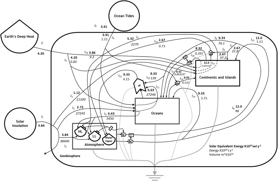
Figure 1. An Energy Systems Language “white box” model of the Geobiosphere tracing the SEE, input from each of the three primary sources (circles) and showing how they interact to support the exergy flows of the system (solid lines with arrowheads). The interconnections among the SEE sources and the system components, i.e., atmosphere, oceans, and continents, show the SEE sources required for the secondary emergy flows of the Geobiosphere (i.e., the labeled pathways) as defined in Table 1. SEEs are given in bold, exergy flows in italics, and water volumes in plain text.

1.1 Emergy and its importance

Emergy is a scientifically powerful yet an often poorly understood concept that has great importance in understanding many important problems in accounting for the health and integrity of ecological systems (Campbell, 2000; Berrios et al., 2018), and in the analysis and understanding of causality in all kinds of systems (Odum, 1971; Odum, 1996). Emergy is important because success in the evolutionary competition among systems and designs depends on maximizing the emergy flow captured by a system and then being fed back to bring in more available energy (Odum, 1996; Campbell, 2001). For this reason, “emergy” in the form of maximum empower (i.e., maximum emergy flow measured in solar emjoules or sej/unit time) provides a unified, comprehensive, thermodynamically controlled decision criterion by which the behavior of all systems is ultimately constrained. The fact that maximum empower and not maximum profit is nature’s decision criterion makes it critical that more people become familiar with emergy evaluations and how to use the results of these analyses in decision-making. Thus, managers responsible for the success of their systems should have as a primary goal the development and implementation of policies that will maximize the empower (emergy/unit time) flowing through their systems, and thereby maximize their system’s functional integrity or health, i.e., the system’s competitiveness in the competition among all systems to capture the available energy of resources from the Geobiosphere (Odum, 1996; Campbell, 2000). The relative empower generated provides managers a general criterion to use in choosing among alternative systems. The problem of maximizing the empower captured always occurs within the context of a set of forcing functions impinging on a system from the next larger system, and since these forcing functions are always changing at faster or slower rates, the maximum power should not be thought of as a fixed endpoint to be attained but rather as a constant state of seeking this goal, thus maximum empower is a moving target (Campbell, 2001). This property of maximum empower makes it essential to consider the temporal boundaries of the system under evaluation. Quantifying the flows of available energy (i.e., exergy) in a network over time provides data on system condition to support decision-making by managers responsible for the wellbeing of their respective ecological and socioeconomic systems. Some examples of the use of the Energy Systems Theory in the management of ecological and social systems are found in Odum et al. (1998) in the “Environment and Society in Florida” and in Campbell et al. (2005a) that provide examples of the application of Energy Systems Theory in the management of a US state. Kangas (2004) gives examples of the use of the Energy Systems Theory and other key articles in the development of a new discipline of ecological engineering. Campbell et al., 2014a provide a discussion of the use of the Energy Systems Theory in the analysis of energy use in the United States from 1900 to 2011 with a particular emphasis on understanding the “Great Recession of 2008”.

1.1.1 Emergy and empower

Emergy is of universal importance because the transformation of energy potentials underlies and is responsible for all actions that have been observed in the universe. Emergy has been operationally defined (Odum, 1996) as the available energy (i.e., the exergy)¹ of one kind that has been used-up, both directly and indirectly, in the process of producing a product (i.e., a quantity of mass, energy, and information) or a service (i.e., the provision of a flow of mass, electricity, human labor, horsepower, and information). Emergy is a quantitative property of the evolution of system networks over time that can be derived directly from the requirements of the first² and second³ laws of thermodynamics and the proposed fourth⁴ law or the maximum empower principle and its corollaries, e.g., the proposed fifth law or the principle of energy hierarchy⁵ (Odum, 1996). As mentioned above, emergy derives its explanatory and predictive power from the fact that maximizing empower (emergy flow) in a process, system, or network has been hypothesized to be nature’s decision criterion (Lotka, 1922a; Lotka, 1922b; Odum, 1996; Campbell, 2000; 2001). Thus, in the competition among systems (mineral, human, animal, ecological, or socioeconomic), success at all hierarchical levels of an organization depends on maximizing empower at the level within the universal hierarchy of natural phenomena at which the system exists and this condition radiates or propagates to all other levels in the hierarchy.

The suite of emergy inputs, or the emergy signature of forcing functions driving system behavior, is derived from the system operating at the next higher level of the organization, and these inputs are constantly changing, whether at a faster or slower rate. As a result, a system at the level in the hierarchy receiving these inputs will be constrained to adjust its structure and function to outcompete its competitors (i.e., other system designs) in capturing the available energy in the signature. This must be true if a system is to prevail in competition or fails to persist as part of the mix of systems that survive. In general, persistence is only possible under the constraint to maximize empower because of the variability present in systems at all hierarchical levels. This variability opens the way for redundancy to be built into systems, for which additional choices provide the flexibility to maximize empower at other times and places; therefore, entities that can only persist under one set of forcing functions may prevail under a future forcing regime. Nature through its laws does not respect species, per se, only the functionality of a species is respected, which is demonstrated by its ability to maximize empower within the context of the system’s current emergy signature (Campbell et al., 2009).

Based on the arguments given above, it is easy to see the importance of knowing the expected change in emergy flow (empower) through a system before choosing among possible alternatives or changes to be made to the system. More exactly, maximizing empower is nature’s decision criterion, and we ignore such natural laws at our own peril. While a manager who understands the importance of the arguments given above to the future of a system will surely want to know the changes in the emergy flow that may result from a management action that has been authorized, making the decision to evaluate these changes will lead to a set of further considerations.

1.1.2 Emergy is an accounting quantity

First, unlike many easily measurable holistic indicators of a system's condition, such as the body temperature of a human being the summary measure of health, emergy cannot be measured directly. Emergy is not an observable state variable; therefore, there is no place in the universe where an instrument can be placed to make a direct measurement of the emergy of a stored quantity or flow. Emergy and changes in emergy flow can only be measured using an accounting process, for example, the available energy that is used in the production process of a product or service can be tracked and then summed over the time and path used to form the output (Tennenbaum, 1988). By contrast, the output or product of these exergy transformations is observable and can be directly measured in energy, mass, or information units. Also, the available energy or exergy of a quantity is not a state variable because its value is defined relative to a background energy level or its environmental context, which can change, and therefore it must be specified by measuring the quantity, e.g., the geopotential energy of water is measured by the elevation of water on the landscape relative to the sea level, the specified ground state. Once the background reference has been chosen, the available energy of an entity can be quantified in a uniform manner, i.e., measured relative to the background. Thus, the major emphasis in emergy quantification has always been laid on the rules that are used to perform the accounting, because maximum emergy flow is a predictive universal quantity that can only be measured through an accounting process (Brown and Herendeen, 1996; Odum, 1996). These accounting rules can be expressed in somewhat different terms depending on the method used to quantify the emergy of storages and flows for example, Le Corre and Truffet (2012) and Le Corre and Truffet (2015) formulated the rules somewhat differently, but in a consistent manner with past rules, to allow making emergy calculations in a network using the graph theory. This focus on the accounting rules has, at times, led to some confusion and sometimes a tendency toward blind obeisance due to the failure of investigators to keep in mind the deeper meaning of emergy, i.e., what it is.

1.1.3 The deeper meaning of emergy

The deeper meaning of emergy arises from its identity as a thermodynamically controlled variable that quantifies nature’s decision criteria within the context of evolutionary competition. Specifically, hypothesizing to maximize the empower captured by a process or system to determine its success in the competition among alternative system designs that are competing for the use of available resources, given that all processes are operating at maximum power efficiencies. An exergy flow from a given system or component to an exploiting process can allow the capture of more energy in available resources, because it provides a higher quality feedback (i.e., entities with higher emergy per unit of available energy, seJ J⁻¹) than an equivalent quantity of feedback from other components with which it is in competition. The underlying assumption for such comparisons to be valid is that all the processes are operating at their maximum power states. Under this condition, more effective feedback can do more work per unit of available energy dissipated. This is a fundamental prerequisite in determining the existence of an increase in the emergy of a component or process in a system, i.e., exergy with higher quality per unit quantity must have an increased ability to do useful work⁶ in its system, with all other factors being equal. This condition serves as a fundamental constraint on the calculation of emergy and on its accounting rules, i.e., the quality, or the ability to do work, of the quantity of available energy must increase, if the emergy delivered per unit exergy of the component or process increases, given that all processes are operating at their maximum power points. This profound connection between maximizing emergy flow and success in the evolutionary competition for resources and the role of high-quality available energy feedback in this maximization is explored in this article as the basis for promulgating an emphasis on the deeper meaning of emergy as a guiding context for performing emergy calculations and for applying the existing rules of emergy algebra to carry out these calculations (Tennenbaum, 1988; Brown and Herendeen, 1996; Odum, 1996) more effectively. In this article, the existing emergy accounting rules are modified to incorporate some important aspects of the emergy accounting methods mentioned in Odum (1996) and later considered further by Brown (2005) and Brown and Brandt-Williams (2011), but these possible innovations, though pointed out, are not fully applied in most emergy accounting studies. In this article, we expand the rules of emergy accounting using a meta framework that includes the broader temporal and spatial emergy flows required to account for the development of system structures essential to bring about the emergy flows of concern in an evaluation. This approach often results in including temporal boundaries that are required for the creation of certain items that are broader and those usually included in a typical emergy analysis. The effects of this approach can be most clearly seen in the role of the emergy required for the creation of biomass accumulations in determining present emergy flows that are required for different plant processes, such as growth and reproduction. Other examples of the meta framework are seen in the inclusion of the emergy required for the education and training of workers in the evaluation of human labor use in economic systems. The foremost macroscopic modification of the accounting rules proposed here is that the first consideration in all emergy analyses should be the recognition that there must be a fundamental connection between the ability of an entity to do work in its system and its emergy intensity or transformity and vice versa. In this regard, the emergy accounting rules should lay their primary emphasis on an exact accounting, neither overcounting nor undercounting, of the emergy required for creating an entity and understanding the actions that will result from its use.

1.2 Objectives of this study and preliminary information

The reader should note that critical material and ideas for understanding this study are given in Supplementary Material A and B, which should not be neglected in obtaining an understanding of the origins of the material presented in this article. First, the effects of the radiation of the emergy methodology on the accounting process are considered (Supplementary Section A1.0—Radiation of the Emergy Methodology). Next, the development of the emergy methodology during the period from 2002 to 2016 (from H.T. Odum’s death to the publication of the four key baseline articles) is considered in Supplementary Section A1.1—Environmental Accounting: Past Problems and Current Advances. In the context of this study, the SEE basis for the Earth system was reexamined to ensure greater methodological consistency in Supplementary Section A1.2—A reexamination of the solar equivalences of the Earth’s primary exergy inflows is presented. This reexamination of the baseline yielded data that further supported our estimate of 12.0E24 seJ y⁻¹ as the value for the SEE baseline for Earth in Supplementary Section A1.3 giving further support for 12.0E+24 seJ y⁻¹ as the value of the SEE Geobiosphere baseline. Finally, differences between the determinations of the baseline carried out by Brown and Ulgiati (2016) and Campbell (2016) are examined and a commentary on the significance of the differences is given in Supplementary Section A1.4—Differences between the Geobiosphere models used by Brown and Ulgiati (2016) and Campbell (2016).

The immediate objectives of this study are (1) to reexamine the emergy evaluation of the flows of air and water within their thermodynamic context in the global Geobiosphere and to develop a meta framework with expanded spatial and temporal boundaries within which the rules used to calculate emergy flows for a given system can be applied more accurately, i.e., more exactly, in determining all the exergy required for a particular flow or storage; (2) to propose self-consistent solar equivalence ratios for tidal exergy dissipated in oceans and by Earth’s deep heat flow based on refined baseline calculations (Supplementary Section A1.2); (3) the data given in Campbell (2016) are reexamined to reaffirm the value calculated for the SEE baseline of the Geobiosphere (Supplementary Section A1.3), and we present a “white box” Energy Systems Language (ESL) model for calculating the exergy in the most important secondary and tertiary wind and water emergy flows of the Geobiosphere; and (4) to carry out the new calculations of the transformities of the major secondary and tertiary emergy flows using the “white box” framework for applying the calculation rules proposed under (1) mentioned above. A refinement of the flows of materials on Earth, such as rocks and minerals, is not considered in this article but can be found in a new United States Environmental Protection Agency (USEPA) publication mentioned below.

2 Advances in modeling the Geobiosphere

In this section, we consider the primary theoretical advances presented in this article that are related to the determination of the secondary emergy flows of the Geobiosphere. The first innovation is to examine the Geobiosphere and develop calculation methods for the major secondary exergy flows within an explicit “white box” model of the major planetary processes. The “white box” modeling approach has been used in emergy analyses in earlier studies when details of an interacting system were of interest (Odum, 1983; Odum, 1994). For example, see Figure 25-9, simulation of a coastal county with an oyster fishery from Boynton (1975). In this article, a white box model will be applied in modeling and calculating the secondary (Figure 1) and tertiary exergy flows of the Geobiosphere (Section 4). The second advance is to examine the premise that methodological self-consistency in determining spatial and temporal boundaries is the primary characteristic required to ensure a valid emergy evaluation. If followed, this approach will guarantee that future emergy analyses will be transparent, self-consistent, and reproducible.

2.1 A “white box” model of the Geobiosphere

The theoretical model used by Odum (1996) to calculate transformities for the secondary and tertiary emergy flows of the Geobiosphere is shown in Figure 3.2 of Odum (1996). In this model, all emergy inputs, solar insolation, Earth’s deep heat, and tides are connected to all system components: air, ocean, and crust, which are, in turn, all connected to one another. Odum’s premise for the calculation of the transformities of flows in the global web of processes follows from this model, i.e., in the global network, everything is assumed to be connected to everything else, thus the total inflow of solar equivalent exergy (formerly emergy inflow) to the Geobiosphere is required for all pathways in the model. This is a “black box” model, and the details of the interactions among sources and components in the model were not specified or evaluated by Odum (1996). Campbell (2000) and Campbell (2016) recognized that while this model might be valid in the long run, it may not be valid on the scale of annual processes that occur over periods of approximately 1 year, which is the scale upon which many transformities are calculated and most emergy evaluations are carried out. The ESL model of the Geobiosphere given in Figure 1 shows the major connections within the global network and how the primary inputs: S, solar exergy; E, exergy of Earth’s deep heat; and G, exergy of ocean tides interact to produce the secondary planetary emergy flows. Table 1 includes first-order estimates of the transformities of these global flows in the notes, which can be calculated from the flows given in Figure 1; see Supplementary Section 2.3.

Table 1

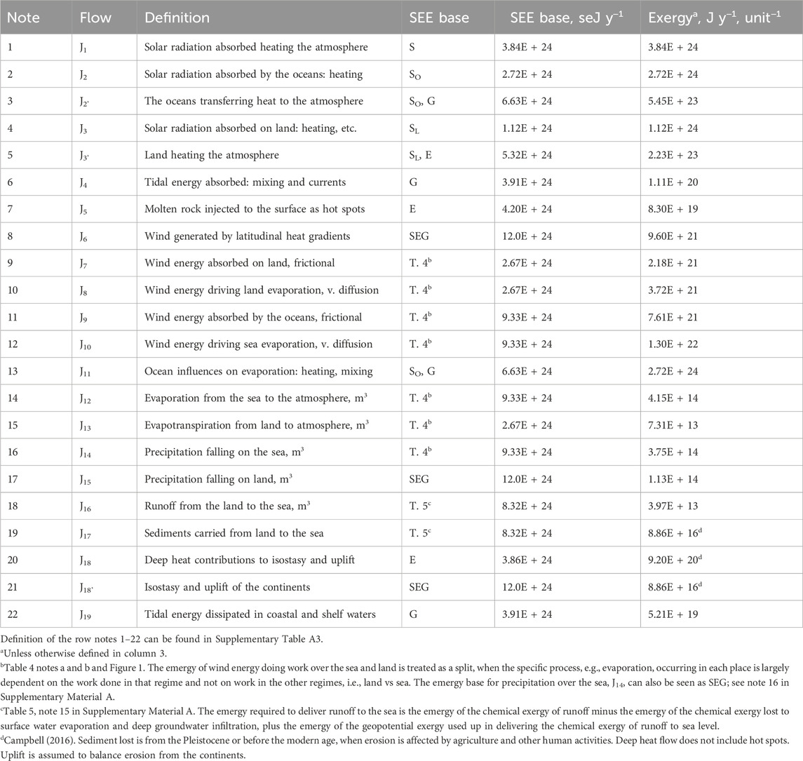
Table 1. The solar equivalent exergy (SEE) base for the major primary and secondary exergy flows of the Geobiosphere (Figure 1), where S is the exergy of solar radiation, E, is the exergy of earth’s deep heat, and G, the exergy of the gravitational attraction of the Moon and sun causing the ocean tides. Oceans constitute 70.95% of Earth’s surface area and the land 29.05%. The SEE base for the global flows is explained in the text.

2.2 Evidence for relationships shown in the “white box” model of the Geobiosphere

The ESL model in Figure 1 shows the primary SEE inflows supporting the major secondary exergy flows of the Geobiosphere on the time scale of 1 year. The model pathways are defined in Table 1 and here below. Although some secondary flows require the entire Geobiosphere baseline, as hypothesized by Odum (1996), others may not. By diagraming and defining the connections within a simplified web of the primary and secondary planetary processes, the connectivity of the network can be explicitly defined compared to the “black box” model used by Odum (1996). In Figure 1, flows J₁, J₂, and J₃ are the primary inflows of solar radiation that are absorbed by the atmosphere, oceans, and earth, respectively. If the atmosphere, oceans, and earth are all passive receptors, nothing other than solar energy (S) is required to cause this heating. The flows, J₂ and J₃, represent heating of the atmosphere over oceans and land, respectively. In this case, both the solar radiation to cause the initial heating and the presence of the oceans and earth to reradiate heat and warm the atmosphere are required for these processes; thus, these flows require the fractions of solar exergy, S, falling on land or water and the emergy input from E or G, respectively. The role of G in heat transfer from the surface of oceans may not be immediately apparent. However, tidal energy influences the heating and cooling of oceans through mixing cooler bottom waters to the surface, lowering the temperature there and decreasing heat transfer to the atmosphere. While tidal mixing often affects surface temperatures in coastal and shelf areas (Tokinaga and Xie, 2009), it may also be important in mixing deeper ocean waters⁷, thereby lowering the surface temperature and reducing heat transfer to the atmosphere. Also, tidal exergy, J₄, directly affects oceans where it is dissipated in mixing and through tidal currents, mostly in the shelf and coastal areas, and also in deep oceans, especially near sea mounts (Egbert and Ray, 2000).

An additional, direct input of exergy from the mantle to crust that was not considered by Campbell (2016) and Brown et al. (2016a) is the molten rock or magma, J₅, emerging as “hot spots” interspersed over the oceans and continents. The formation of hot spots is assumed to be due to plumes of magma arising from somewhere in the mantle and being driven by the same gradient of the Earth’s deep heat that drives uplift and isostasy (Morgan, 1971). Although there has been much debate over the depth in the mantle at which these flows originate (Kerr, 2013a), the physical evidence indicates that their origin within the mantle is below 660 km or the boundary between the upper and lower mantle (Smith et al., 2009) and possibility as deep as the core–mantle boundary (Kerr, 2013b). In the mantle plume hypothesis, hot spots arise from the dynamics of the mantle alone, thus the SEE basis for hot spots is E alone.

2.3 Generation of secondary flows in the Geobiosphere

Solar heating is differentially distributed over Earth, as shown in Figure 1, where the heat gradient between the higher level (HL) and lower level (LL) latitudes is shown. The first major class of secondary planetary energy flows, i.e., the winds are generated by the pressure differences between the atmosphere at high and low latitudes, causing global atmospheric circulation or winds, J₆. The winds are a secondary energy flow generated on a planetary basis; thus, all primary solar exergy inflows contribute to their formation, and the SEE base for the winds is S, E, G, or 12.0E+24 seJ y⁻¹. Wind energy flows intersect with the planetary hydrological cycle through mediating evaporation from the land, J₈, and from the sea, J₁₀. Wind energy affects evaporation from the water surface by transporting water vapor away from the surface, thereby maintaining the water vapor gradient and to a lesser degree by disturbing the water surface, with winds increasing the surface area and further enhancing evaporation. Evaporative processes require the entire baseline of the Geobiosphere, since they are mediated by the actions of the wind. The calculations of emergy driving vertical diffusion and frictional work over land and sea and their exergies were determined using the data from Boville and Bretherton (2003), who provided a means to separate the work done by the wind in driving vertical diffusion from that done in frictional work on the surface. As already mentioned, wind is also absorbed over the land and water surfaces, J₇ and J₉, respectively, where it supports tertiary exergy flows doing work on land, e.g., erosion, and on water, i.e., generating waves and currents. Influences of waterbodies on evaporation from oceans, J₁₁, include solar heating of the water surface modified by tidal mixing, which provides a vast amount of heat to drive the hydrological cycle, but it double counts the wind emergy supporting evaporation from the sea. The global hydrological cycle is shown by the next five flows, which are given as volumes of water in 1E+14 m³. The cycle begins with flow, J₁₂, evaporation from the sea to atmosphere, followed by flows, J₁₃, J₁₄, J₁₅, and J₁₆, which are, respectively, evapotranspiration from the land to atmosphere, precipitation falling on the sea, precipitation falling on land, and runoff from the land to sea. The next three coefficients refer to the earth cycle of uplift and subsidence, with J₁₇ showing the exergy of sediments carried to the sea (Campbell, 2016), J₁₈ giving the contribution of deep heat to drive isostasy and uplift continents, and J_18’ giving the exergy required to support isostasy and uplift the land mass of continents, which, over a long time, is assumed to balance the exergy of erosion, e.g., over millions of years (Campbell, 2016). Finally, flow J₁₉ gives the tidal exergy dissipated in coastal and shelf waters.

Only the known major pathways supplying substantive amounts of SEE to a global process over a period of approximately 1 year are included in Figure 1. In each emergy evaluation, the investigators are responsible for determining the forcing functions and components that are relevant for answering their research questions. Thus, not all pathways may be included initially in an analysis, and missing pathways that are essential or important on the scale chosen for an emergy evaluation may have to be evaluated to complete a particular study as they are revealed. For example, when planetary systems or processes are evaluated over longer time scales (e.g., >10,000 years) other factors that are relevant at those scales must be included in the analysis (Campbell, 2016).

3 Methods

Consider the definition of emergy in Odum (1996) as a starting point for deliberations on the emergy methods presented in this article: “EMERGY is the available energy of one kind of [energy] previously used up directly and indirectly to make a service or product. Its unit is the emjoule (Odum, 1986; Odum, 1988; Scienceman, 1987).” In this article, the deeper thermodynamic meaning of emergy and emergy methods as they are connected to the proposed 4th law of nonequilibrium thermodynamics defined as the maximum 4th empower principle⁸ (Odum, 1996) and the modifications to these methods that are required to accurately determine the transformities of the secondary and tertiary exergy flows of the Earth’s Geobiosphere are presented.

3.1 Energy systems language diagrams

The primary tool developed by Odum (1971), Odum (1983) and Odum (1994) to understand and model systems of all kinds is the ESL. Odum (1996) extended the ESL and the models derived from it to characterize and simulate the variations of emergy in all kinds of systems. The ESL is a diagrammatic language in which all symbols and relationships have mathematical definitions. It is a universal language that uses an open set of symbols to add a thermodynamic (energetic) and kinetic context to the representation of systems and their interactions. Odum (2007) extended the ideas set forward in the seminal book Environment, Power, and Society (Odum, 1971) to include the insights from the Energy Systems Theory and emergy analysis that developed during the intervening 30 years. In this article, the ESL is used to construct models of the secondary and tertiary available energy (exergy) flows of the Geobiosphere and their concomitant emergy flows. The ESL and its use have been extensively documented and illustrated in Odum (1983, 1994) and many additional publications, thus further description and explanation will not be repeated in this article.

3.2 What is emergy?

Although emergy has been defined above using the definitions in Odum (1996), it is sometimes easiest to understand a complex quantity like emergy by stating what it is not. Emergy, per se, is not a quantitatively observable or directly measurable quantity, i.e., there is no place in the universe where one can measure emergy with an instrument or sensor. Nevertheless, it is qualitatively observable in the range of properties that exists in all things. For example, the element carbon appears in many forms of increasing “quality,” i.e., emergy density and transformity or specific emergy (emergy intensity)—e.g., peat, lignite, subbituminous coal, bituminous coal, anthracite or amorphous carbon, graphite, and diamond describe a series of materials of increasing quality or transformity for the element carbon, all of which are not necessarily directly connected. As the potential to do work or the special properties of an entity increase along a chain of exergy transformations, the emergy of that entity must also increase. In some cases, increased emergy and the concomitant ability to do work is manifested by the special properties that an item, often a mass, has when compared with other variations of the same material. For example, diamond is a form of concentrated carbon like coal, but it is not generated from coal, rather it is formed from carbon under conditions of extreme heat and pressure deep in the earth, and as a result, it is resistant to chemical reactions and has the highest thermal conductivity of any natural material, which makes it useful as a cutting tool. Although diamond is not derived from coal, because of its properties, one would expect it to have a much higher transformity or specific emergy than that of coal, and in fact it does, 4.9E+04 seJ J⁻¹ or 1.42E+09 seJ g⁻¹ for coal (Odum, 1996; Campbell and Ohrt, 2009) versus 3.4 E+10 seJ g⁻¹ for diamonds found stored ubiquitously in deep earth (∼180 km below the surface) as determined by estimates of changes in global seismic wave velocities (Garber et al., 2018) and a rough estimate of 6.07E+19 seJ g⁻¹ for the diamonds extracted from earth (Haggerty, 1999; Janse, 2007) during roughly the last 5,000 years, or since recorded human settlement.

3.2.1 Determination of emergy

The emergy required for any item at a point in time can be quantified, if the production process for that product or service is known. This quantification is performed by integrating the available energy transformed directly and indirectly in the process that was responsible for the development of that item with its special properties. Because the transformation of available energy occurs within the milieu of evolutionary competition among processes, when a product emerges from this competition as the “winner,” that product will be of higher “quality,” i.e., be of higher transformity, in that the item will have special properties; e.g., it will be rarer, or it will have a greater capacity to do work (i.e., a higher empower density) than it did before the available energy was transformed and subjected to the competition among production processes in making the item. The emergy required for any item can be quantified by summing up the transformations of the available energy used up, directly and indirectly, in the production process after converting all the different kinds of available energy input to units of the same kind, e.g., to solar joules (Odum, 1996). In this case, the solar emjoule (sej) is the unit of emergy, where the prefix “em-” denotes the past use of exergy in the production process.

3.2.2 Transformity is a universal measure of quality

Solar emergy is usually taken as the base for determining transformities or the emergy required per unit of exergy flow (sej J⁻¹). Using transformities, the relative quality of all things can be measured and compared on a universal scale by summing up the solar emjoules required to produce any storage or flow within a system and then dividing by the joules of exergy in the product. This ratio, the emergy per unit of exergy (sej J⁻¹) is called transformity, which is a universal measure of quality⁹ (Odum, 1996).

The EST indicates that all production processes are constrained by the operation of the maximum empower principle (Odum, 1996; Campbell, 2001) so that to remain competitive in the long run, the emergy flows generated by the feedback from the process to its system must be, at least, as great as the emergy required for the generation of the process or product in the first place. This condition is enforced by the unavoidable evolutionary competition among entities and processes, which ensures that the entities or processes that fail to generate greater empower flow in their networks will be outcompeted by their rivals that do. Figure 7.8 in Odum (1994) demonstrates this condition with mathematical models of competition among the systems where feedback is mediated by linear, autocatalytic, and hierarchical processes.

3.2.3 The meaning of an increase or decrease in emergy

While emergy is not a directly measurable quantity, it is always associated with quantities that are measurable, e.g., the enthalpy of a biomass, such as a mass of fish eggs, and if that physical quantity is removed or destroyed, the emergy associated with it is also removed or destroyed (Odum, 1996). A common misunderstanding about emergy is the failure to recognize that the emergy per unit or the transformity of a quantity must be a direct measure of the quality of that product or its service, e.g., it must be a measure of the work that a storage, flow, or process can do in its system, and the rules for calculating this work must meet this constraint. For example, the emergy of a female fish will increase with an increase in length; however, even at the maximum length, its emergy will continue to increase, if its fecundity increases with age. Once the length and fecundity (i.e., the special useful property of the female fish) reaches the maximum, the emergy of the fish and, by extension, her transformity will no longer increase, regardless of the available energy transformed to maintain the fully developed female fish and its eggs. This understanding of emergy as an accounting quantity that tracks the relationship between the quality or transformity of a product and the exergy transformed to attain that product is seen in the rules for simulating emergy given in Odum (1996). His accounting rules used in simulation do not allow the emergy of a fully formed product to increase indefinitely, even though exergy still may be used to maintain the form of the product against entropic degradation. This is true because the transformity of an item must be an exact measure of the work that an entity can do in its system.

3.2.4 Determining the emergy base for a system by concentrating resources in space and time

It is clear from the ESL models in Odum (1996) that the emergy inflowing to a local system from other areas or other times is to be counted in the emergy base for that local system, i.e., this additional emergy flow is counted along with the share of the Geobiosphere emergy received by the local system’s area (Figure 3.7 in Odum, 1996). The total emergy inflow to the system in the present is responsible for the order and organization being produced there, i.e., the order created within its defined spatial and temporal boundaries. A river flowing across the boundary of a territorial system is an example of emergy supplied to the system through the spatial concentration of renewable resources from outside the system’s boundaries. Imported minerals, fuels, goods, services, and people are all valuable resources that bring emergy into a system from other areas and times to augment the emergy that can be used to produce order and organization in the system under evaluation at the present time. Fossil fuels are a clear example of resources formed at an earlier time that are being used in the present to support the system structure and function, and thus all agree that they are to be counted in the emergy supporting a system under evaluation. With the publications of Campbell and Lu (2009, 2014a) and Campbell et al. (2011), the necessary time delay for the formation of human knowledge and experience prior to the possibility of its application in operating a system was the basis for proposing that educational attainment of the population be considered as part of the emergy supporting the system, e.g., in the United States. In the present study, the temporal separation between resource formation and its application to support system operations is allowed on even shorter time scales than was previously considered, when determining the emergy basis for transpiration of various vegetation types.

The time scale for an evaluation of network energy and material flows in most emergy evaluations is >1 year. In this regard, resources generated on the scale of 1 year or less can be double counted, if the inputs are coproducts. However, if resources require longer times for their generation, the temporal separation might be great enough that these resources created in the past should be counted in the emergy supporting the exergy flows of the system in the present. For example, this new rule was applied to calculate the transformity of transpiration in several types of ecosystems of the world. Specifically, the time that it takes to generate biomass with its spatial structure was quantified as part of the emergy base for evapotranspiration in systems, i.e., those systems that take several years or longer to generate the biomass required to support the evapotranspiration that is realized in the present year. For example, if the contribution of biomass structure to annual crop growth falls within the 1-year time boundary of the evaluation, it would not augment the emergy basis for evapotranspiration. However, a tropical rainforest with structural biomass that takes 30 years or longer to be formed would have the emergy base for this structure quantified and prorated over the replacement time of the forest to determine the support required from the forest biomass for rainforest evapotranspiration within the temporal boundary of a single year.

3.2.5 The emergy associated with different exergies in water

In addition to better quantify the concentration of emergy from different spaces and times in determining the emergy basis for a system, the study of hydrological systems over a long period of time (Odum, 1996; Odum et al., 1998; Campbell, 2003) has made it clear that a refinement is required in accounting for the emergy associated with the various forms of exergy in water. Odum (1986) originally defined emergy in terms of its association with the available energy of a storage or flow. Initially, the conceptualization of available energy in emergy evaluations focused on a single type of energy, such as the energy of combustion in biomass, even though biomass also has another form of available energy associated with it, i.e., the available chemical potential energy in the bonds of its constituent compounds that can be used in chemical reactions. While this form of available energy in biomass might be relevant in certain chemical processes, it is, in general, irrelevant in the use of biomass as food in a trophic web. Exergy is a concept like the available energy that was applied by Szargut et al. (1988) for use in evaluating chemical and industrial processes, and in this approach, care is taken to quantify all the forms of available energy (i.e., exergy) that exist in a quantity. Both available energy and exergy indicate the energy potential available to do work against a ground or background state, which must be defined. Odum (1971, 1983, p.105) originally used the term potential energy to refer to the aspect of energy that is used up in performing work, which he associated with the thermodynamic term “availability”. Afterward the term available energy was used to refer to this concept in the literature, but in Odum (1996), emergy was defined based on exergy instead of on available energy. However, this change in definition has only been partially integrated into the emergy methodology.

As mentioned above, in all cases, emergy must be associated with an underlying quantity of exergy; therefore, it is logical to assume that each source of exergy in an entity has an available energy (potential to do work) associated with it. This must be true because emergy must track the capacity to produce order and organization in a system, and this capacity can only be and always is derived from the transformation of an energy potential, i.e., a quantity of available energy that has the potential to do work. Furthermore, the two different forms of exergy in water do different kinds of work in the system, and the work done is not always mutually exclusive. The existence of two forms of exergy in a single quantity does not satisfy the definition of a coproduct, which is defined as two different quantities with non-substitutable functions and uses that are products of the same production function. In this case, two different capacities to do work, i.e., exergies, reside in the same quantity of water. A different accounting scheme is required for this situation. A logical solution is to assign to each quantity, i.e., the geopotential or chemical potential energy, the emergy required to give a quantity of water that exergy. This accounting scheme leads to the potential for the two different types of exergies in water to interact over the landscape with the geopotential energy, in general, serving as the means of concentrating the chemical potential emergy at places within a watershed. The complex interactions of these two different types of exergies and their associated emergy on the landscape was considered by Romitelli (1997). The most important result of this accounting concept is that both the chemical potential energy delivered to a location and the geopotential energy of water used in transporting and concentrating water flows at that location contribute to the transformity of water entering the sea or arriving at various locations in the watershed.

These proposed changes in the rules for calculating the emergy supporting a system are required because according to the fundamental accounting rule emphasized above, emergy must be a measure of the capacity to produce order and organization within the defined spatial and temporal boundaries of a given system. Since each type of exergy in water is a separate and independent source for creating order and organization, both must be considered when they are mutually reinforcing such as in the case of landscape water flows. The emergy inputs to a system must be fully documented in accounting to accurately reflect the capacity for organizing the system inherent in the inputs. Thus, both the emergy of resources concentrated in a system from different space and time domains and the emergy associated with different exergies found within a single material must be fully accounted for in determining the emergy base of a system. Strict balances are maintained in first-law diagrams of the underlying energy measures upon which emergy is based on, but emergy itself is not a conservative quantity nor could it be or still track the transformations of available energy required for current exergy storages and flows. Instead, emergy is an accounting quantity that tracks the concentration and transformation of energy potentials that have the capacity to produce order and organization when used in a system. Therefore, emergy always follows the underlying energy potentials as they are formed or removed by destruction, use, or transfer out of the system. The underlying energy quantities always satisfy the conservation principle and are observable and measurable, whereas emergy is defined by exact accounting rules, but it is neither directly observable nor measurable as explained above.

3.3 The emergy accounting rules applied within the context of the deeper meaning of emergy

The present rules of emergy accounting are primarily designed to make accurate determinations of the emergy of any product or service by avoiding double counting. They are important because, as pointed out above, the quantification of emergy is fundamentally an accounting problem, and thus its value and the accuracy and comparability of results depend upon the consistent application of the rules and assumptions used in its determination. The rules of emergy algebra (Scienceman, 1987; Brown and Herendeen, 1996; Odum, 1996) as given in Li et al. (2010) are as follows:

(1) For a system at steady state, all the emergy inflows to a production process are assigned to the outputs.

(2) When an output pathway splits into two or more pathways of the same type, the emergy input is assigned to each “leg” of the split on the basis of its fraction of total available energy or material flow on the pathway; therefore, the transformity or specific emergy of each branch of the split is the same.

(3) For a process with more than one unique output, i.e., coproducts, each output pathway from the process carries the total emergy input to the process, i.e., the entire emergy required for a process is also required for each of its functionally different products.

(4) No emergy input to a system can be counted twice. Thus, if an input or feedback flow to a component is derived from itself, i.e., it carries emergy already counted in the emergy required for the component, then the input or feedback flow is not added to the emergy required for that component, i.e., input emergy is not double-counted. A corollary to the prohibition against double counting (i.e., counted twice) is that coproducts of the same production process when reunited cannot be added to obtain an emergy input greater than the original emergy input. Thus, when adding emergy inflows or outflows that are coproducts, only the largest one should be considered.

The primary purpose of the emergy accounting rules is to allow the accurate determination of the emergy of a product or service within a network of available energy transformations. The meta framework proposed in this article states that regardless of the exact form of the rules for the calculation of emergy, the general context within which the rules are carried out is the same, i.e., exergy use always increases the quality of the product of or service provided to the system given that the product is being made in its process of formation; however, these actions will occur with greater or lesser efficiency, which results in higher or lower transformity products as a result. For processes making equivalent products, a lower transformity for an equivalent product indicates a higher efficiency process, and it is the one that will ultimately maximize empower in the network (Tilley, 2015). Therefore, attaining maximum empower in a network is an endeavor of the whole system that is also hierarchical in its nature, so while less-efficient processes are ultimately less competitive, they are also secondary contributors to the competitiveness of the whole network. The main result of applying a deeper understanding of emergy is to balance the prohibition to avoid double counting with an equal weight on avoiding undercounting, the reason being that we want to obtain more accurate assessments of the emergy required for an item, which should be closely related to its action and effectiveness upon use in the network. Often the missing piece in this chain of causality is the verification of the improvements made in system structure or function that result from the use of exergy in the system. The goals of developing and demonstrating a more accurate accounting method will require more research to document the relationships between increasing transformity and the resulting greater performance observed for all kinds of quantities and processes within their networks. In general, in scientific studies, too little attention has been given to documenting the changed relationships that result from the use of exergy in a system. This concern to avoid undercounting manifests itself in two ways: one is through the separate accounting for the actions of different exergies in creating the same product or service, when both are used together. The second is through performing a more exact accounting of the emergy contributions made from temporal and spatial regimes that are separated from the annual and local scales of the production of products and services in the evaluated system by times longer than the period of evaluation or territories beyond the local system boundaries.

4 Results

The primary results of this emergy accounting study are presented in the form of a set of evaluated models with pathways identified and quantified in a series of tables with explanatory notes, where calculations of the transformities of the secondary and tertiary exergy flows of the Geobiosphere derived from wind and water can be found along with the necessary assumptions and supporting references. The article also presents a new approach to quantifying exergy inputs, the meta framework, which more exactly documents past exergy inputs required for quantifying some system storages and flows. The ultimate result of this study will be to allow emergy accountants to produce more accurate assessments of the wind and water emergy inputs to many systems and document other inputs that are dependent on stored emergy more accurately, e.g., products of some stored biomass and educational expertise. Once the solar equivalent exergy for the primary emergy inflows has been established (Brown et al., 2016), the emergy of the secondary exergy storages and flows can be calculated within the system boundaries of the Geobiosphere. In Section 2.1, a “white box” model of the Geobiosphere was presented as an ESL diagram, which shows the major secondary exergy flows of the system and their interactions with explicit formulations as documented in Sections 2.1 and 2.2. Since the model is documented extensively in Table 1, these descriptions will not be repeated in the text, except as specifically called for as a context for discussion. A similar approach using ESL diagrams documented with detailed notes and calculations is used to present the evaluation of transformities of the major tertiary exergy flows of the Geobiosphere, as presented in this section.

4.1 Secondary flows: wind

The white box model of the Earth’s Geobiosphere as presented in Figure 1 outlines the major interactions of the primary exergy inflows to the Geobiosphere, showing how exergy is transformed and secondary emergy flows are developed. The emergy basis for these flows is given in Table 1. The largest secondary exergy flow of the Geobiosphere is the wind, and for this reason, we will consider ways to determine its transformity first.

4.1.1 Transformity of wind energy determined from a general circulation model of the atmosphere

Wind energy dissipation in the atmosphere below the 100 mb surface [i.e., the elevation of the planetary boundary layer (PBL)] was determined from the general atmospheric circulation model of Wiin-Nielsen and Chen (1993); see Supplementary Figures A1, A2, Table A4. Their estimates ranged from 0.95 W m⁻² (Northern Hemisphere summer) under conditions shown in Supplementary Figure A1 to 2.95 W m⁻² (Northern Hemisphere winter) under conditions shown in Supplementary Figure A2. Supplementary Table A4 shows the transformities of the wind in the PBL and Geobiosphere boundary layer (GBL), i.e., the layer below the 900 mb (≈1,000 m) surface for maximum and minimum estimates of summer and winter winds taken from the general circulation model of Wiin-Nielsen and Chen (1993) and for maximum and minimum estimates of the amount of kinetic energy in the GBL that are given by Ellsaesser (1969).

4.1.2 Determination of the transformity of the wind from observations of average wind velocity

The transformity of the wind was determined from the global average wind velocity measurements taken at 10 m over the continents and oceans from 1998 to 2002, as compiled by Archer and Jacobson (2005). They reported global average velocities at 10 m, V₁₀, of 6.64 m s⁻¹ over the oceans and 3.28 m s⁻¹ over land. These average velocities, V₁₀, were substituted into Eq. 2 given in Supplementary Material A after first converting them to the geostrophic velocity, V_g, or the wind velocity predicted at the top of the boundary layer, GBL ≈ 1,000 m. A range of plausible values was substituted into Eq. 2 for determining the factor relating V₁₀ to V_g and for the geostrophic drag coefficients over land and water to estimate the transformity of the global wind (Table 2).

Table 2

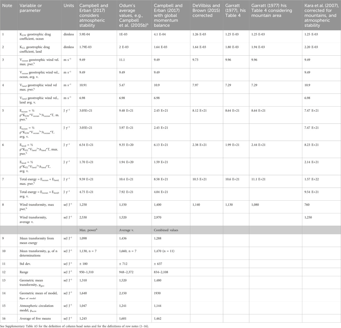
Table 2. Estimation of the transformity of the wind from models and empirical data. Constants used in the calculation: ρ, density of air, 1.225 kg m⁻³ at 1 atm pressure, and 15°C; A_ocean, ocean surface area, 3.62E+14 m²; A_land, land surface area such as freshwater lakes, 1.48E+14 m²; average ocean wind velocity, OV₁₀, 6.6 m s⁻¹; and average land wind velocity, LV₁₀, 3.28 m s⁻¹ (Archer and Jacobsen, 2005), both measured at 10 m; number of seconds in a year, T = 3.16E+07 s y⁻¹. Geobiosphere solar equivalent exergy baseline, GEB, is 12.0E+24 seJ y⁻¹. See explanatory notes appended below.

Table 2 shows the results of 11 different determinations of the transformity of the global wind calculated from seven different studies that were based on different assumptions about the factors relating V₁₀ to V_g. We used these studies to determine the best values for the geostrophic drag coefficients to use over land and water. Column notes a–h in the table explain the origin and derivation of the numbers in the columns representing each calculation method used by the different authors and the assumptions supporting their calculations (see Supplementary Table A5). The estimates are divided into two sets as noted in the table, one representing the minimum transformity found at the maximum power generated by the wind using the assumptions of the method and the other representing the average value for the method. The row notes, Numbers 1–7, explain the variables and parameters, which are defined in Column 2. Row 8 reports the average transformity of global wind energy found by each calculation method for average and maximum power conditions. Rows 9–15 present statistical analyses of the determinations, such as the mean, standard deviation, and range, the geometric mean velocity, and the geometric mean of the model (i.e., the formulae for wind energy given in Notes 5–7). The maximum power estimate of the transformity of the wind from the global atmospheric circulation model of 1,047 seJ J⁻¹ was combined with the four maximum power estimates of the wind transformity from the empirical determinations (Table 2) to give an estimate of 1,245 seJ J⁻¹ for the transformity of wind energy dissipated in the GBL at maximum power. Using NCAR’s CAM2 model, Boville and Bretherton (2003) have provided another analysis of the transformity of the wind that allows us to distinguish the wind energy dissipated in frictional effects on the surface (1,226 seJ J⁻¹) from the wind energy dissipated in diffusion (715 seJ J⁻¹).

4.1.3 The tertiary exergy inputs to the oceans derived from the wind

The major tertiary emergy flows derived from the wind are shown in Figure 2 and include waves on the ocean surface, waves transmitted to the shore, geostrophic wind-driven currents (i.e., currents at the scale of the ocean basins), Ekman layer transport (local surface currents affected by the Coriolis force), Stoke’s transport (local currents moving in the direction of the wind), and near-inertial motions. In Figure 2, the wind blowing on the ocean surface, J₁, generates waves, J₃, and drives geostrophic currents, J₄, as well as Ekman transport, J₅. Some of the wind energy passing over the oceans, J₂, continues to be dissipated over the land. Wave energy drives Stokes drift, J₆, and generates near-inertial motions, J₇. Water movements driven by Stokes drift interact with Ekman transport, J₈, to augment the wind energy basis for total surface water flow and because of the Coriolis force alters its direction away from a 90° displacement from the wind direction as expected for surface currents. In other words, the current direction is commonly displaced less than 90° from the wind direction. Surface currents in the Ekman layer interact with the wind-driven wave field, J₉, to help move wave energy shoreward, J₁₀. Some fraction of the wave energy is dissipated in the surf zone, J₁₁; here, we assume it is 100%, when the entire continental shelf is considered. Wave energy is also dissipated in the oceans as white caps in breaking, along with other processes, J₁₂. The energy dissipated in friction by the wind energy driving water movements—i.e., geostrophic currents, J₁₃, Ekman transport, and Stokes drift, J₁₄, wave energy transmitted to the shore, J₁₅, and near-inertial motions, which appear in the total, J₁₆—is assumed to balance the exergy inflows to these storages over a year’s time. The exergy flows of some ocean currents are evaluated in Figure 2 and are shown in blue italics. Geostrophic currents, J₁₇, and Ekman transport, J₁₈, are affected by the Coriolis force with the direction of the flow shown by arrows directed into or out of the page, indicating the flow in the Southern and Northern Hemispheres, respectively. Stokes drift, J₁₈, is wave-driven transport that moves in the direction of the wind part of which J₁₉ augments Ekman transport. The combined surface water flow (Ekman transport augmented by Stokes drift) is shown as, J₂₀, and this combined water flow helps transmit wave energy to the shore.

Figure 2

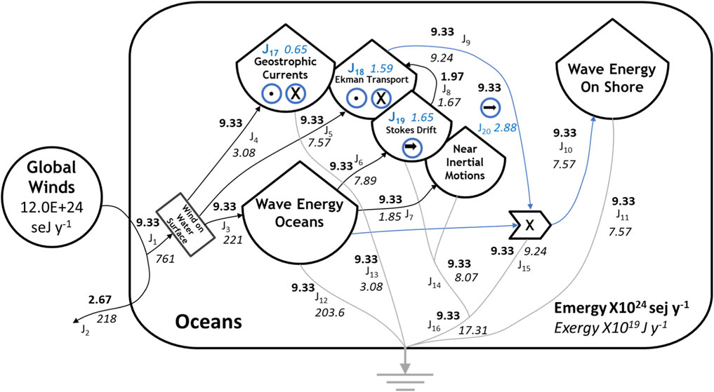
Figure 2. An Energy Systems Language “white box” model of the world oceans tracing the SEE input from the global winds (circle) and showing the way that wind work on the ocean surface that generates tertiary emergy flows in the oceans. The major storages and flows of exergy generated by the wind energy dissipated in the oceans are shown in the model, but only the exergy flows are evaluated in this study (Table 3). Water flows are shown in blue with the arrows directed into the page (X) or out of the page (•), showing the effects of the Coriolis force in the Southern and Northern hemispheres, respectively. Stokes drift (➡) moves water in the direction of the wind. Emergy flows (seJ y⁻¹) are given in bold, and exergy flows (J y⁻¹) are in italics.

4.2 Secondary flows: water and the hydrological cycle

The white box model of Earth’s Geobiosphere (Figure 1) outlines the major interactions of the primary exergy inflows to the Geobiosphere, showing how the secondary emergy flows related to water within the hydrological cycle are developed. The secondary exergy flows related to the hydrological cycle are the second category of major biophysical flows generated by the primary SEE inputs to the Geobiosphere. The determination of the transformities of the secondary flows of the hydrological cycle is considered in this section. Some of the transformities calculated as in the notes to Table 1, such as the quotient of the SEE and exergy flows on the pathways, may be somewhat different from the values obtained from the tertiary analysis of global wind and water flows described in Figure 2 and Table 3, and in Figure 3 and Table 4 (see the footnotes to Table 1).

Table 3

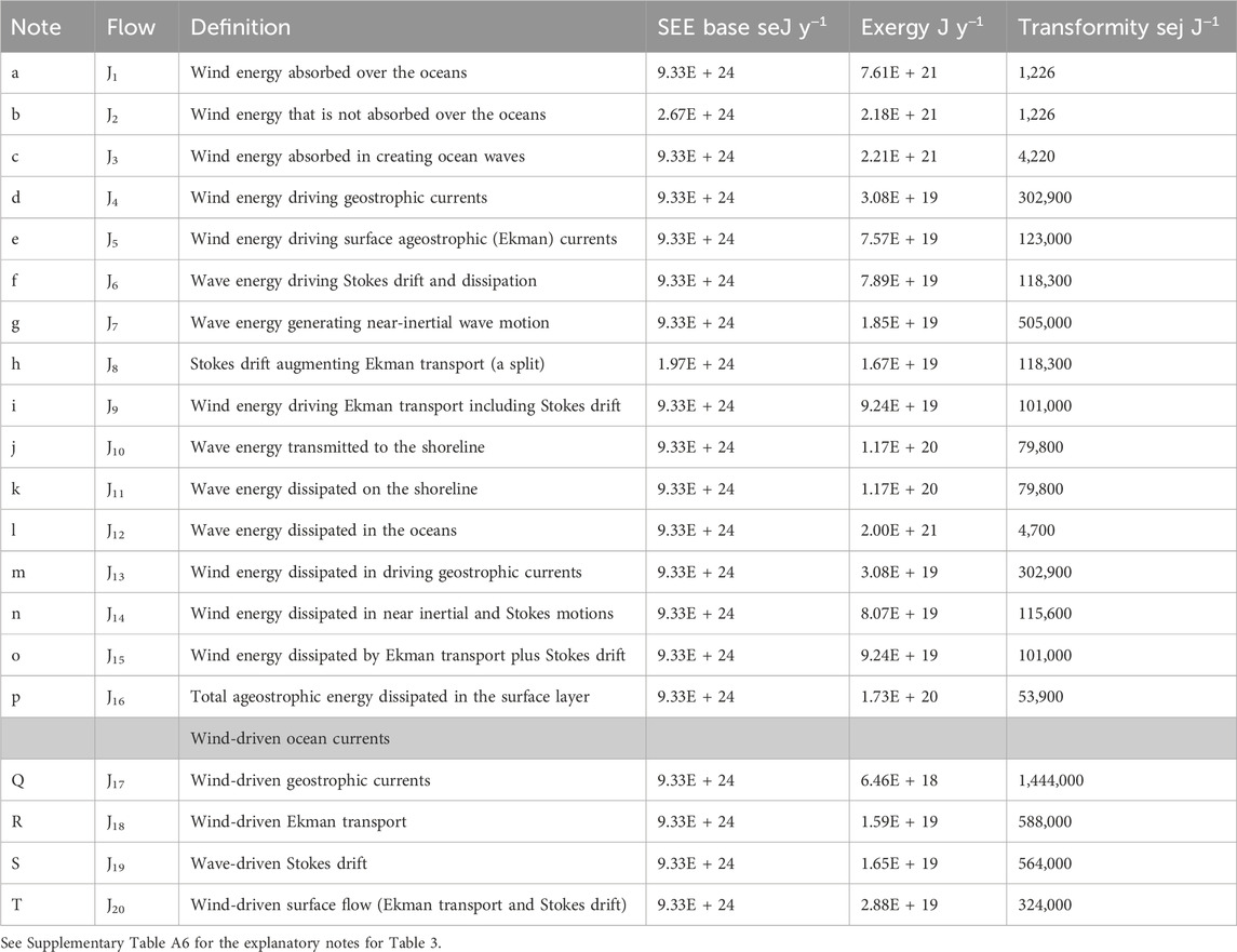
Table 3. The emergy basis for the tertiary exergy flows in the world oceans are generated by wind (a secondary flow) and are used for the empirical determination of the drag coefficient over the oceans (Kara et al., 2007). They result in the oceans absorbing a larger fraction of the total wind energy. Definitions of the pathways shown in Figure 2 are given in this table along with the annual flows of the exergy of the wind in the world oceans driving waves and surface currents of various kinds and showing the SEE basis for these flows. Also, the exergy and transformities of some surface currents and motions are shown. All flows are coproducts, and coproducts are recombined in several flows.

Figure 3

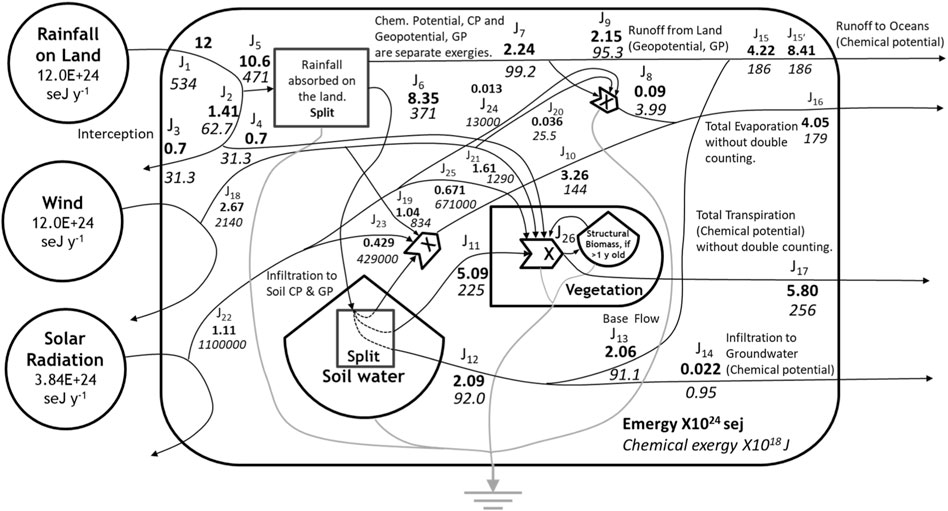
Figure 3. An Energy Systems Language “white box” model of the terrestrial hydrological cycle tracing the SEE input from precipitation falling on land, the wind dissipated over land, and solar radiation incident on the land (circles) and showing the emergy and chemical exergy of tertiary water flows generated in the terrestrial hydrosphere. Table 4 gives the definitions of the pathways, storages, and the annual flows of emergy, volume, mass, and chemical and geopotential exergy in each pathway, as well as, the transformities of the flows of chemical and geopotential exergy and their specific emergy. See Supplementary Table A7 for the explanatory notes for Figure 3.

Table 4

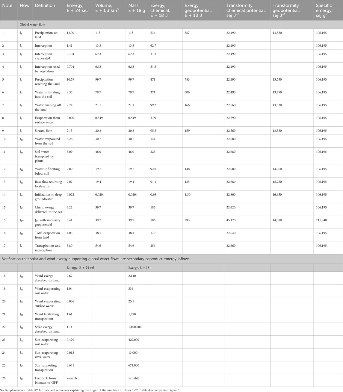
Table 4. Definitions of the pathways and storages in Figure 3; the annual flows of emergy, volume, mass, and chemical and geopotential exergy are given on each pathway, as well as, the transformities of the flows of chemical and geopotential exergy and specific emergy. The emergy and flows of solar and wind exergy supporting the water flows of the hydrological cycle are also given.

The water flows of the hydrological cycle were determined using the three methods described in Supplementary Section A3.0—Methods for calculating the secondary available energy inputs to the Geobiosphere: Supplementary Section A3.1—Equations governing the wind, Supplementary Section A3.2—Methods for determining the exergy of water flows in the hydrological cycle, and the method for evaluating the transformity of the tides, which is described in the Supplementary Section A3.3—Methods for determining the transformity of tides. Supplementary Section A3.4 describes Calculating transformities for the secondary and tertiary exergy flows of the Geobiosphere. In Supplementary Section A4.0—Uncertainty in the calculations, we consider three kinds of uncertainties that are relevant to the calculations of the secondary and tertiary available emergy flows of the Geobiosphere. Supplementary Section A4.1 considers Uncertainty in the determination of the fraction of wind energy dissipated over the oceans.

4.2.1 Quantification of the global hydrological cycle

Supplementary Table B1 gives 10 global hydrological budgets reported in studies carried out from 1974 to 2015, nine of which were reported in Marcinek (2007). A 10th study by Rodell et al. (2015) was added, and the mean, standard deviation, coefficient of variation, and the maximum and minimum of these estimations are reported in the table. The global flows of water in the hydrological cycle used in this study are from Adler et al. (2003), assuming a hydrological balance over the annual cycle. The statistical parameters from this study were compared to similar values obtained by analyzing the 10 global budgets mentioned above (see the last row in Supplementary Table B1). The estimates of Dai and Trenberth (2002) were chosen to complete the hydrological cycle by supplying a value for global runoff from the land to oceans. After accounting for infiltration into the deep groundwater, this number is 39.7 1,000 km³ y⁻¹. Assuming closure of the hydrological budget, these choices lead to estimates in 1,000 km³ y⁻¹ of 113, 73.1, 39.9, 414.9, and 375 for precipitation on land, evaporation on land, runoff to the sea, evaporation over the sea, and precipitation over the sea, respectively.

4.2.2 The tertiary available energy flows of the terrestrial hydrological cycle

The tertiary emergy flows of the terrestrial hydrological cycle derived from precipitation on land are shown in the model given in Figure 3, and the data sources, values, assumptions, and methods of calculation for these flows are given in Table 4. The exergies of the tertiary emergy flows derived from the rain were determined based on studies in the literature, and the descriptions of these calculations and the sources for the values used are given in Table 4, following the network of relationships described in Figure 3.

The ESL diagram of the tertiary flows of the hydrological cycle (Figure 3) is briefly described as follows: the diagram shows that rainfall, J₁, from Figure 1 can be intercepted, J₂, before being absorbed by the land surface, after which it can evaporate from the surface of the vegetation, J₃, or it can be absorbed and can contribute to supporting the productive processes of the plants, J₄. The precipitation not intercepted, J₅, reaches the ground surface and can be absorbed there. Precipitation absorbed by the land surface is handled as a split between water that infiltrates into the soil, J₆, and that which runs off at or close to the surface, J₇. Runoff includes the surface water flows, which are subject to evaporative losses, J₈, and contribute to stream flows, J₉, e.g., rivers. The fate of water that infiltrates into the soil, J₆, is shown by another split that occurs within the soil. This split includes water that is evaporated from the soil, J₁₀, water that is absorbed by vegetation, J₁₁, and water that infiltrates deeper into the ground, J₁₂. Water that infiltrates below the soil can return to the streams and rivers as base flow, J₁₃, or can infiltrate into the deep groundwater, J₁₄. The chemical potential energy delivered to the sea is J₁₅, if only the concentration of chemical potential energy in the hydrological network is considered in determining the emergy of river water delivered to the sea (Table 4). However, if the geopotential energy used up in bringing the river water to sea level is also considered, the value is given by J_15’. Total evaporation from the system, J₁₆, includes intercepted water and surface water evaporated along with evaporation from the soil surface. Total transpiration, J₁₇, includes the portion of intercepted water contributing to plant growth and plant transpiration. Flows J₁₈ to J₂₅ quantify the inputs from the sun and wind used to support evaporation and transpiration. These flows are not counted in the emergy base for the water flows because they are not larger than the inputs from the hydrological cycle, and if included, they would double count the emergy inflows supporting the water cycle (see Table 4).

4.2.2.1 Estimating interception in the ecoregions of the world

Interception is one of the tertiary water flows listed in Figure 3 and Table 4. Interception is the rainfall captured by the vegetation, e.g., tree canopy, stems, and forest floor, before it can seep into the soil; it has not been commonly evaluated in past emergy assessments of the hydrological cycle. Supplementary Table B2 gives an estimate of the average value for interception in the global hydrological cycle using values from the ecoregions of the world as defined by Schlesinger and Jasechko (2014).

4.2.2.2 Estimating the contributions of structural biomass to transpiration

In Figure 3, flow J₂₆ represents the feedback from stored plant biomass to facilitate plant production processes such as transpiration. These flows are evaluated in Table 5 and 6 where the emergy base for long-term structural biomass and the transpiration of vegetation found in the ecoregions of the world (Schlesinger and Jasechko, 2014) is determined (Table 5). Table 6 shows the emergy base for transpiration from Table 5 and estimates the water transpired by the ecoregion. These values are reported and are used to calculate the transformity and specific emergy of transpiration of the major vegetation types by the ecoregion.

Table 5

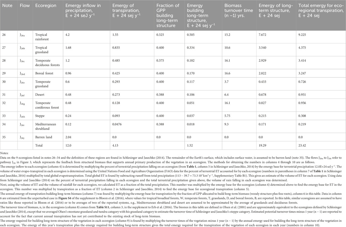
Table 5. Determination of the emergy base for long-term structural biomass and transpiration of vegetation found in the ecoregions of the world as defined by Schlesinger and Jasechko (2014). Data on transpiration as a percent of evapotranspiration and the percent of terrestrial precipitation falling on each ecoregion were used to determine the emergy required for transpiration of vegetation in the ecoregions.

Table 6

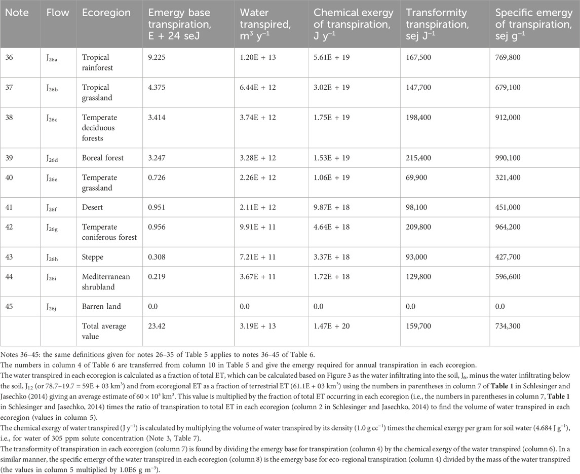
Table 6. Determination of the transformity and specific emergy of transpiration of the vegetation found in the ecoregions of the world as defined by Schlesinger and Jasechko (2014). Transformities and specific emergy evaluations include the effects of accumulated biomass and are rounded to the nearest 100 seJ.

Some important transformities derived from this work and rounded to the closest 10 seJ J⁻¹ are precipitation and the related surface water flows: chemical potential energy of 22,490 seJ J⁻¹ and geopotential energy of 13,530 seJ J⁻¹. The specific emergy of precipitation is 106,200 seJ g⁻¹. The transformity of water evaporated from the soil surface or transpired by plants is 22,680 seJ J⁻¹, and the transformity of total evapotranspiration which includes that from the surfaces of the soil, plants, and fresh water is 22,640 seJ J⁻¹, while the transformity of all water used to support plant growth such as transpiration and intercepted water absorbed by plants is 22,660 seJ J⁻¹. The number for evapotranspiration (22,680 seJ J⁻¹) is a base number applicable to processes with structure built on the scale of 1 year, such as annual crop growth. For ecosystems with vegetation that require at least several years to develop, the structure required to facilitate transpiration, the transformities of plant processes such as transpiration and gross primary production (GPP) are higher (Tables 5, 6), e.g., the transformity of tropical rainforest transpiration is estimated to be 167,500 seJ J⁻¹, which is more than 7 times higher than that of annual crops). A complete description of the calculations required to determine all the transformities and specific emergy evaluations of the tertiary exergy flows of the hydrological cycle is given in Tables 4–6 and in the explanatory notes associated with these tables.

4.3 The emergy of water flows in the hydrological cycle estimated from global storage and turnover time

Table 7 gives values for the major storages of water in Earth’s hydrological cycle as identified by Babkin et al. (2003). Four estimates of the volume of the major water storages on Earth are reported in Supplementary Table B3 for comparison to Babkin et al. (2003). The sources for the water volumes, turnover times, solute concentrations, and density of the various storages of water in the hydrosphere are given in Table 7, and the exergy, mass flux, and exergy flux are calculated from these data. The specific emergy evaluations and transformities of the water fluxes are also determined from the data and shown in the table as are the estimates of the value of the natural capital of the various water storages. The key values that result from this analysis are the transformities of predominantly fresh groundwater, 311,000 sej J⁻¹, fresh water in lakes, 478,000 sej J⁻¹, water in swamps and bogs, 1,100,000 sej J⁻¹, and permafrost, 87,000,000 sej J⁻¹. Among the natural capital storages of water in the Geobiosphere, permafrost has the highest value, 1.20E+29 sej, followed closely by permanent ice cover, such as that found in the Arctic and Antarctic, 1.16E+29 sej. The next largest natural capital water storage in the Geobiosphere is predominantly fresh groundwater, 1.68E+28 sej.

Table 7

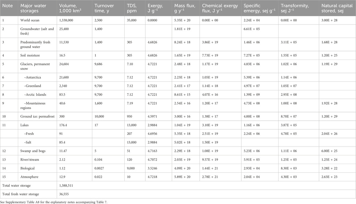
Table 7. Transformities and specific emergy evaluations of the annual flows of water passing through the major storages of the hydrosphere and the stored natural capital in the Geobiosphere. The emergy required for all flows is 12.0E + 24 seJ y⁻¹, as all flows and storages listed are ultimately dependent on terrestrial precipitation. Most numbers are from Babkin et al. (2003) and given in Shiklomanov and Rodda (2003) except as noted.

4.4 Comparison of new calculations of the secondary and tertiary emergy flows of wind and water with earlier values in Odum

The primary existing source of calculations for secondary and tertiary emergy flows of the Geobiosphere is Folio #2 of the Handbook of Emergy Evaluations (Odum, 2000a). In this small pamphlet, Tables 2 and 6, respectively, report emergy analyses of the energetics of atmospheric circulation and ocean circulation, both of which are considered in this study. Supplementary Table B4 gives the solar emergy base, the exergy flows, and the transformities associated with each of the flows in Odum (2000a) that were reexamined in this article along with some recalculations of existing flows and new calculations of missing flows that were performed as additional examples to check the existing estimates. Tables 3 and 4 in Odum (2000a) present an analysis of the exergy and transformities of latent heat and continental rainfall as a function of height (these data are reported in the “Altitude” class in Figure 4 and in Supplementary Table B4). These functions are combined, checked, and where necessary recalculated in Supplementary Table B5. Odum (2000a) also considered the emergy of Earth processes, but a reexamination of these and other analyses in Odum (2000a) is left for a later time. The table notes document the data sources and assumptions used in making the calculations. Unlike in the folios, mathematical errors in the original calculations are noted and corrected in the table. Recalculated values are marked with a (') and new values that represent alternate estimates using different data or those that consider flows that are not formerly determined are indicated by an (*). In both cases, an additional superscript is added for each new calculation.

Figure 4

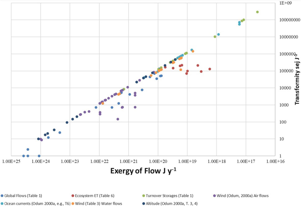
Figure 4. Plot of all transformities (sej J⁻¹) of the secondary and tertiary exergy flows (J y⁻¹) of the Geobiosphere that were evaluated in this study. The transformities of the flows are plotted by functional analysis groups as defined below. The functional groups refer to tables in this article and in Odum (2000a) and are as follows: global flows, Table 1; ecosystem ET, Table 6; turnover of storages, Table 7; wind flows (Odum, 2000a), his Table 2 and Supplementary Table B4; ocean currents, Odum (2000a), Table 3 and Supplementary Table B4 in this study; wind-driven flows, Table 3 in this study; and “Altitude” in Odum (2000a), Tables 3 and 4. The data plotted in this figure are summarized in Supplementary Table B6.

4.5 Transformity as a function of exergy flows in the Geobiosphere

Data on the secondary and tertiary exergy flows of the Geobiosphere and the resulting transformities associated with these flows are compared and summarized using a master plot of transformities of all the phenomenon examined in this study vs exergy flow (Figure 4). The data for this figure are reported in Supplementary Table B6. The well-defined diagonal in this figure is created by Geobiosphere processes that require the entire baseline for their formation. Off-diagonal flows are based on regional processes, have temporal components affecting their formation, or have other formation conditions, requiring less than the full Geobiosphere baseline to produce the flows, e.g., molten rock ejected to Earth’s surface (J₅ in Table 1).

4.6 The relationship of the transformity of ET with exergy flow for ecoregional functional groups

The group of red dots in Figure 4 give an analysis of ecosystem evapotranspiration, ET, examined by ecological functional groups. These systems form a group for which exergy flow and transformity appear to have a different relationship from the general pattern observed for global processes. These relationships are examined in detail in Supplementary Table B7 and Figure 5 below, where the ecoregions of the world are divided into three functional groups: tropical systems, temperate systems, and a constructed category, i.e., conifers and Mediterranean shrublands. Each of the three groups includes a grassland ecoregion (Supplementary Table B7) with steppe included in the constructed category. Figure 5 shows that the transformity of ET in tropical ecoregions has a strong logarithmic relationship (R² = 0.9938) with exergy flow, whereas both temperate ecoregions and the constructed category have strong linear relationships with exergy flow. The relationships between exergy flow and the variables account for the departure or conformance of the relationship between transformity and the exergy of ecoregional transpiration with the diagonal. The relationship between the transformity of tropical rainforest ET and its exergy flow is closest to the relationship of transformity to global exergy flows in global processes.

Figure 5

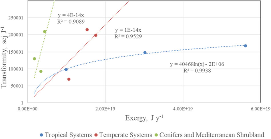
Figure 5. A plot of the transformity of transpiration in the ecoregions of the world (Supplementary Table B7) as a function of exergy flow. The vegetation falls into three functional groups defined by different relationships of transformity with exergy flow. The transformities of tropical systems have a logarithmic relationship of transpiration with exergy flow, whereas the transformities of transpiration in temperate systems and in the constructed category “Conifers and Mediterranean Shrublands” exhibit more linear relationships with exergy flow.

5 Discussion

The emergy basis for systems is better defined by expanding the time frame of its quantification to include the work done by the system in the past that is required for the creation of components that are actively used in the present evaluation, e.g., vegetation biomass created over many years in the past is used in creating plant processes in the present. The operation of the maximum empower principle is observable in the hierarchy of quality observed in all phenomena, but its defining quantity, emergy intensity, is not directly measurable, as it depends on the history of past use of available energy. For this reason, the rules of emergy accounting in space and time become very important and must be continually tested and refined to increase the accuracy of emergy quantifications. This article focuses on the further development and testing of the rules by which the emergy of storages and flows within a system can be determined with greater fidelity to the underlying thermodynamic processes and the time required for their development. In this regard, we consider the importance of self-consistency in the use of the emergy methodology as the primary characteristic of a cogent emergy evaluation, and therefore ways to ensure that an emergy evaluation will be self-consistent and become of paramount importance. Building on the firm foundation of the four articles to determine a new planetary baseline for emergy analyses, we have taken the next step in verifying and revising the transformities and other emergy evaluations per unit value of the secondary and tertiary exergy flows of the Geobiosphere that will be required to perform self-consistent and cogent emergy evaluations of all of Earth’s phenomena. Specifically, in this article, we have documented the emergy flows of the secondary and tertiary exergy flows of wind and water as they are derived from the network of exergy flows in the Geobiosphere. These revised data provide the input required to perform more accurate emergy evaluations.

5.1 Application of the primary rule of emergy accounting

The primary rule of emergy accounting superseding all other rules is that when an increase in the emergy of a component or process in a system is determined by the chosen accounting method, i.e., the quality or emergy per unit of the evaluated quantity increases, then this quantity must have an increased ability to do useful work in its system. Also, the converse of the rule must be true. This rule places the emphasis on obtaining an accurate accounting of all past use of exergy required for the product or service being evaluated, neither over nor under counting exergy in the evaluations. In pursuit of greater accuracy in accounting, the separation distance between the use of the required emergy in space and time is reduced, but it cannot be equal to or smaller than the evaluation limit for an annual evaluation. In the limit, the evaluation can consider as potential inputs all entities that are separated by more than the period of the evaluation, usually 1 year in most emergy analyses. Brown and Brandt-Williams (2011) called for consideration of both space and time domains in evaluating the emergy inputs to all systems. This rule accomplishes this, although other alternatives might be put forward. Several examples of the application of this rule are given above, but perhaps the most significant for overall emergy evaluations is the requirement to consider the emergy of educational attainment in the evaluation of systems such as human work. The integral of the emergy required to accomplish the past years of schooling (Campbell and Lu, 2014b) is required in the evaluation of national systems to allow the accurate determination of the emergy basis for national economies and to determine the emergy balance in the equity of trade.

5.2 The evolution of the emergy methodology

The International Society for the Advancement of Emergy Research, also known as the Emergy Society, was formed in July 2007. Soon after this organization was established, which included a Standards Committee, the society recognized the tension that would inevitably develop between establishing a standard method of analysis and the intellectual creativity required by a young methodology that continues to be under development. Campbell et al. (2005a) identified this and several additional problems that the emergy methodology was facing at that time, and chief among them was the problem of disagreement on the value of the planetary baseline to be used in emergy accounting. Now, the baseline questions have been resolved for the time being with the publication of the four strong articles mentioned in the Introduction section that converge on the value of 12.0E+24 seJ y⁻¹. Furthermore, the additional data and analysis in Supplementary Material A of this article further strengthen the evidence supporting this number.

A solution of the conflict between intellectual creativity and standardization of the emergy methods can be resolved through insights in this article because the fundamental characteristic of the measurement of emergy depends on the fact that it is an accounting quantity, and therefore, its quantification depends on the suite of accounting rules chosen to govern the evaluations. As a result, the most important characteristic in determining the emergy of an item is the self-consistency of the accounting method. Furthermore, the validity of the quantification of emergy can be judged by how accurately the emergy of the item represents the observed properties and actions of the item in the system of which it is a part. The integrity of any proposed rules can be judged by their conformance to scientific laws and the principles of the Energy Systems Theory (Odum, 1983, 1994). To further ensure the self-consistency of the methodology, an open access database of transformities and other emergy evaluations per unit factors could be set up, using a blockchain accounting model (Tapscott and Tapscott, 2016). The entries would include the emergy per unit factors (also called “Unit Emergy Values” or “Emergy Characterization Factors”) and the ESL model required to produce each item, such as the references for all sources and antecedents. The use of the database would be free after registration, but all users would be required to add their new calculations, ESL diagrams, and documentation to the website once these are complete. The Emergy Society offers a dataset last worked on by Tilley et al. (2012) that can be accessed from http://www.emergysociety.com/emergy-society-database/ and might be suitable to build upon.

Most recently, the USEPA has just completed a new database (De Vilbiss et al., 2024) of Emergy Characterization Factors (ECFs), i.e., emergy per unit values or transformities, which if expressed in energy units, can serve as a basis for creating consistent emergy analyses and evaluation models (https://www.epa.gov/water-research/uev-library). This database not only covers most of the air and water flows given in this article but also provides data on Earth processes and other systems important for completing emergy analyses. This new publicly accessible database of ECFs, if adopted internationally, will greatly improve the consistency and reliability of emergy evaluations around the world. Science is not fixed and improvements to knowledge are constant, so we still require a system like the blockchain accounting model of database construction proposed above to help emergy evaluation develop at a maximum rate.

5.3 Use of “white box” models of the Geobiosphere, global wind–driven circulation, and hydrological cycle

As mentioned above, Odum (1996) used a black box model to determine the transformities of the global secondary and tertiary exergy flows. An innovation in this article is that we used “white” box models to evaluate the exergy flows of the Geobiosphere (Figure 1), the wind-driven circulation system (Figure 2), and the hydrological cycle of Earth (Figure 3). The primary difference between these two accounting models is that in the former (Odum, 1996), the network is assumed to be completely interconnected, and thus, the entire SEE base for system flows is necessary to support every flow in the network, whereas in the later, the requirements for any flow or process must be traced through the network from the points of use to the points of origin (this study). Some flows in the “white” box system require all the SEE inputs to support them, but other flows do not. The advantage of “white” box models is that they provide a chance to use all the knowledge that we have about a system to obtain a more accurate determination of the system’s exergy flows and the relative transformities of these flows. A disadvantage is that if we increase the information required to evaluate the system, the chance to introduce errors into the calculations increases. Despite the use of different models for the emergy evaluation of secondary and tertiary exergy flows of wind and water, the transformities determined in this article correspond well (Supplementary Table B4) to the transformities determined for some similar flows in Odum (2000a). “White” box models are easier to check for errors because more specific information on the mechanisms of interaction is provided, therefore they are subjected to more verification and subsequent correction, if shown to be wrong.

5.4 Examples of the proposed methods for determining the chemical potential energy of water

Under the method proposed in this article, determining the transformity or specific emergy of an exergy flow in the system requires an estimate of all the types of exergies present in that flow that must be used up in the process of creating it, along with an estimate of the emergy required for the existence of the types of interacting exergies. This new method of accounting for interactions when more than one type of exergy is required for the same flow is applied to determine transformities for water flows in the hydrological cycle. The proposed changes make the determination of the emergy of water more consistent with our knowledge of the two exergies required for a given chemical potential exergy flow to be used at a particular location on the landscape. In this study, accounting for the emergy of water in the hydrological cycle is performed under the assumption that both the chemical potential of the water flow and the geopotential of the same water flow that is used up in the process of delivering the chemical potential in the water to its point of use are required to accurately capture the emergy required for the water flow to be used at a location. For example, the chemical potential energy of fresh water delivered to sea carries both the emergy of its chemical potential and that of the geopotential used up in the process of delivering the water parcel to sea level. Similarly, the emergy of runoff augments the emergy of water pooling in places such as floodplain forests and augments transpiration there, above that supported by local rainfall alone. In both cases, the test of accuracy of the altered accounting scheme is in the observations that the organizing power of exergy flows is greater than expected from the use of the base transformity for chemical potential energy alone. Floodplain forests are complex systems that may be governed by the subsidy–stress gradient as proposed by Odum et al. (1979). The emergy of the chemical potential of water, concentrated there, depends on both local rainfall and on the water transported to that location from higher in the watershed. To determine whether or not the concentration of the emergy of chemical exergy in floodplain forests results in a greater order and organization than is found in an upland forest requires the study of the whole system in all its aspects (biological, chemical, physical, and geological) and may not be indicated by the comparison of a single parameter such as forest productivity, which because of the role of water as a stressor, a subsidy, or both may not tell the whole story (Odum et al., 1979; Megonigal et al., 1997). In the case of the water debouched into the sea at river mouths, the importance of river discharge to maintain the thermohaline circulation of the oceans has been recently demonstrated through model simulations (Huang and Mehta, 2010).

The proposed meta framework of emergy evaluation put forward in this article requires that the assessed value of the emergy of a product or service must be a true reflection of the ability of that entity to do work in its system and vice versa. In other words, if the ability of an entity to do work increases, then its emergy must also increase. If this second condition does not hold, then the method of calculating emergy of an entity must be modified to better reflect the change in its ability to do work in the system. An example of this principle begins with the observation that different types and qualities of plant production are observed in the various ecological regions of the world, and these various forms of plant structure require various time periods to develop to their mature state. Thus, there is a temporal separation between the past use of exergy to create structural biomass and its use in the present to produce the exergy flows associated with various kinds of plant production. This fact leads to the realization that the historical emergy flows that create the structural biomass of plants over periods longer than 1 year (Table 6) should be accounted for as an input in determining the transformity of the present emergy flows of different vegetation types, e.g., transpiration, gross primary production, etc.

5.5 Significance of the proposed changes in determining the emergy required for items

Implementation of the proposed changes in the methods for determining the emergy of items may make a difference in many transformities and may or may not make large differences in the overall results, depending on the specific processes evaluated (i.e., historically, emergy analyses have been extremely robust in the face of errors and omissions). Odum (2000b) examined the ecological–economic process of salmon pen culture in the Pacific Northwest section of the United States and found that the buyer of pen-raised salmon received twice the emdollar value compared to the dollars paid for the fish. The most significant fundamental principle of emergy analysis is the recognition that the most important characteristic of a valid emergy evaluation is self-consistency in the methods and models used to perform the calculations. Odum (2000b) showed that once the salmon are processed and used by consumers, seven emdollars from the outside economy are attracted for each emdollar of local environmental product. In this study and in Campbell (2016), a functional approach to emergy evaluations has been proposed and used. This approach is like the original work on emergy evaluations, which is tied to quantify a series of functional processes creating order and organization in a system within defined spatial and temporal boundaries (Tennenbaum, 1988; Odum, 1996). The thread of self-consistency in these analyses is the tracking and summing of all the directly and indirectly required emergy inflows (i.e., exergy × transformity) necessary to make a new exergy flow.

In this article, we have urged that additional attention be placed on quantifying the extended spatial and temporal boundaries required to account for all necessary inflows producing activities in the present system. From this perspective, determining the emergy of an item is performed by tracing the path of all its inputs and ensuring the independence of each one. Emergy evaluations that are most likely to experience changes in their evaluations are vegetation assessments that include plants with large older biomass accumulations and human systems where the education of people is considered in the evaluation of exchanges. This article focuses on advancing the emergy accounting methodology, clarifying it, and ensuring that more accurate assessments can be made, especially regarding the emergy flows of wind and water.

5.6 Comparison with other methods of determining emergy

In general, determining the emergy of an item requires the identification of secondary and tertiary emergy flows that are responsible for organizing the exergy flow or storage of interest within the system. Thus, the exergy flows that are directly and indirectly used up in producing the exergy of another item or process are determined and then multiplied by their transformities and summed to determine the emergy necessary for creating an exergy flow or storage. Approaches such as the use of primary SEE inflows on a proportionate basis over the surface of Earth, an idea called the “tripartite” by Brown and Brandt-Williams (2011), and using them to assign emergy values would not make sense in the accounting scheme proposed here, although this idea could be used in other accounting schemes. The reason that this method is not consistent with a process-based approach to quantify is that it does not follow identified and verified lines of interaction from the emergy sources to the products made.

Emergy evaluation covers all the sciences, and it was left in a certain state of development by Odum (1996) and Odum and Odum (2000). One point of contention has been the way that Odum characterized the equations for describing changes in emergy over time (i.e., dynamic emergy). Odum’s conceptualization of emergy and of the problem of describing it dynamically was that it is not a state variable and therefore requires a different set of equations centered on the emergy accounting rules to describe its temporal changes accurately. In Odum's (1996, pp. 9–13) view, three phases are required to accurately describe the change in emergy over time. In the first phase, while emergy is being stored, i.e., the emergy of the product is increasing, but the formation process is not yet complete, the emergy of the product increases and this includes the emergy lost to the heat sink in the formation process, as this emergy use is also required for building the product. In the second phase, the product is built and there is no change in its emergy (Odum, 1996, Figures 1–7), and thus the rate of change of the emergy stored is 0. In the third stage of emergy simulation, the product is made but suffers a net loss, either from removal of the product to another system or from the depreciation of the stored product’s mass, i.e., the loss of its ability to do work. In both cases, the stored emergy of the product declines. Odum and Odum (2000, p. 157) make it clear that both changes in the emergy stored or a change in its nature, i.e., its ability to do work, can be responsible for a change in the stored emergy of the product. All emergy calculations are based on a correspondence with a real quantity of exergy represented in the ESL model. The dynamic rules governing the transformations of the emergy in a storage are always subject to these real processes. Emergy has no existence when it is separated from the real quantities (e.g., enthalpy) that it is associated with.

In another case, Odum and Odum (2000) propose a solution for dealing with the question of when a product is fully formed. This is a key question for simulations of the development of a product. In the case of an industrial process, it is apparent when the product is available, e.g., the time when a chair or table built from wood is completed. There is no question about the existence of the product, even though it may be characterized in terms of the quality of its construction, durability, etc. However, the completion of a product within an ecosystem may be somewhat more difficult to determine. Odum and Odum (2000) proposed a solution to this problem by assuming that such products are generated within a spectrum of natural variability that will set statistical boundaries on the quantity of emergy generated in the final product. Despite this modeled solution, there are many quantities in nature where the emergy of a product can be easily determined. For example, the transformity of a female fish will continue to increase, if her capacity to produce eggs increases. This capacity may increase up to the maximum size of the fish. Again, the key to any emergy assessment goes back to the system that is responsible for producing the item of concern. Given the system or item of concern, variables can always be found that capture the development of quality within that item. Theoretical constructs can be chosen when better real variables are not available.

Although models can be created and simulated using Odum’s rules (Campbell et al., 1998), in most cases, these rules do not make simulation easy. In a series of articles, Tilley (2014, 2015) proposed a set of alterations to the Odum equations that make them easier to simulate. In my view, it is valid and reasonable to use different methods to try to get a better understanding of dynamic emergy accounting. Tilley has developed a productive method that has been used by others (Lee, 2014) to investigate important problems such as the role of resource pulses in power acquisition by ecosystems. Tilley’s articles yield interesting insights into the method and possible nature of emergy when viewed dynamically; however, the redefinition of terms in his modeling scheme removes the main constraint on Odum’s definition of emergy, i.e., emergy is not a state variable and requires different rules and a different set of equations for its simulation to be accurately represented. However, despite these rule changes, Tilley’s simulations and analyses give what appear to be reasonable and interesting results.

In conclusion, neither Brown and Brandt-Williams (2011) approach to emergy evaluation using manipulations of the tripartite (solar equivalent exergy baseline) nor Tilley’s redefinition of the rules governing dynamic emergy flows are entirely consistent with the understanding of path-based emergy evaluations put forward in this article. However, these approaches are from the same tree of knowledge as are the proposals for evaluating emergy presented here, and are therefore not incompatible with one another.

5.7 Expansion of emergy analysis of the wind

Wind is a complex quantity that is often the second most important environmental emergy input to a system found on the surface of the Earth. Under certain conditions, it can be the largest emergy inflow, and in other cases, it is responsible for the largest negative environmental impact on system wellbeing, e.g., the effects of wind causing erosion affecting agriculture (Asgharipour, et al., 2020). The properties of the wind are determined by pressure and temperature gradients in the atmosphere, which in turn determine the stability of the fluid and govern its mixing properties. Wind is often considered only superficially in emergy analyses, nevertheless, it can be the most important variable in determining certain environmental impacts, such as land erosion and the vertical mixing and distribution of pollutants. Supplementary Section A5.7.1 considers the effects of atmospheric stability on the transfer of wind energy to Earth’s surface, and Supplementary Section A5.7.2 gives an estimate of the transformity of the energy dissipated in the GBL by wind.

5.8 The choice of the best transformity for wind for a given study

There is uncertainty in all our calculations, especially in the values reported for wind and the calculations made using these values (Table 2; Supplementary Table A3). Nevertheless, all the studies converge on numbers that are self-consistent and give a reasonable approximation even though they may be superseded by more accurate or authoritative values in the future. One understanding that emerges from this examination of the wind and its transformity is that the transformity of wind energy differs depending on the aspect of wind energy that is of interest in a particular study. For this reason, it is important to understand the purpose of wind transformity values that have been calculated in the past and the appropriate value to use for any research project in the future. For example, Boville and Bretherton (2003) showed that wind energy doing frictional work on Earth’s surface (Table 3, notes a and b) has a different and higher transformity (1,226 seJ J⁻¹) than the wind work dissipated in driving atmospheric vertical diffusion (715 seJ J⁻¹). The aggregate work in the boundary layer is a combination of these two values, but consideration of wind exergy may lose this practical context of its application in synthesis.

5.9 The importance of scientific accuracy

Both wind and sun are important and necessary inputs to the hydrological processes of evaporation and transpiration; however, these inputs would double count the evaluation of transformities based on global water flows if included in the calculation of the transformities without first checking to see if they are the largest inputs of emergy to the processes. In Table 4, a comparison of the emergy of flows J₁₉, J₂₀, and J₂₁ for wind and J₂₃, J₂₄, and J₂₅ for sun with flows J₉, J₁₀, and J₁₁ based on the hydrological cycle shows that the sun and wind are secondary sources of emergy supporting the processes of evaporation and transpiration from the soil and vegetation. The feedback from structural biomass to current plant production (e.g., GPP and transpiration) is a necessary input required to account for the variations in the different qualities of plant production, e.g., grasslands vs forests.

5.10 Data choices and uncertainty

The estimates of global precipitation given in Adler et al. (2003) were thought to be the most accurate because they used a combination of low-orbit microwave satellite data and geosynchronous-orbit satellite infrared data adjusted with surface rain gauge observations to make their estimates of global precipitation over land and water as part of version 2 of the Global Precipitation Climatology Project. The estimates of Dai and Trenberth (2002) of runoff from the land to oceans were chosen to complete the hydrological model because they estimated global river flow at the points of discharge to the sea and used several methods to check their estimate. Further discussion of uncertainty in the model can be found in Supplementary Sections A.3.0 and A. 3.1.

Values from Trenberth et al. (2007) in Supplementary Table A2 were not chosen, but they illustrate plausible variations from the generally accepted values. For example, they report a slightly smaller total volume of the world oceans due to an ostensibly more accurate account obtained by using the National Geophysical Data Center’s terrain database with 5-min ocean depth data and land elevations. Other departures from Babkin et al. (2003) seen in Supplementary Table A2 were not used, e.g., the volume of permafrost reported by Trenberth et al. (2007) is markedly lower than that reported by the other three global budgets.

6 Conclusion

The work done by exergy transformed over time and concentrated within the spatial and temporal boundaries of the global system is responsible for the order and organization observed in wind and water systems found within those boundaries. One of the main products of this study is to provide updated values for the wind and water flows of the Geobiosphere, so that they can be used to create more accurate and consistent emergy evaluations. The numbers presented here are self-consistent and have been calculated using common accounting rules and perspectives given in the article, such as the inclusion of resources necessary to quantify emergy storages accumulated from the past use of resources yet necessary to support present flows. An overall plot of the transformities of the wind and water flows evaluated in this study is given as a global comparison plot (Figure 4). Wind and water flows are defined here with functional definitions, requiring specific biophysical processes and the underling exergy transformations with the emergy of the products that they deliver explaining the order and organization observed within the global system. Furthermore, in this study, we propose the use of a meta framework for the determination of transformities. This framework extends the spatial and temporal boundaries for systems that include components that require additional development times to produce important energy flows in the system under analysis. Many ecosystems include components, such as plant biomass and the accumulated knowledge of workers and many others in social systems. The consideration of this larger window to capture the essential exergy inputs to key system components may result in major changes to the results of some emergy analyses. We have presented a functional approach to the accounting problem of determining the emergy required for any product or process using a meta framework or filter for recognizing important inflows that provides an updated analysis of the inputs from the wind and water flows of the global system. Emergy evaluations are accounting problems and the accounting rules and body of values required to determine accurate transformities of emergy flows are key pieces of information to allow emergy accounts to be accurately constructed. These flows are self-consistent and are clarified, extended, and further evaluated in this article. Also, they are consistent with a new USEPA database that provides the potential to create better emergy evaluations throughout the world. From this perspective, the order and organization observed in a system in the present depends solely on the biophysical processes operating within these spatial and temporal boundaries or concentrated there from other spatial and temporal realms and on the useful work (emergy) that they deliver to the organizing processes within a system.

Data availability statement

The original contributions presented in the study are included in the article/Supplementary Materials, further inquiries can be directed to the corresponding author.

Author contributions

DC: Writing–review and editing, writing–original draft, visualization, validation, supervision, software, resources, project administration, methodology, investigation, funding acquisition, formal analysis, data curation, and conceptualization. HL: Writing–review and editing.

Funding

The authors declare that financial support was received for the research, authorship, and/or publication of this article. Partially funded by the United States Environmental Protection Agency, Narragansett, RI, USA, and the Project of the National Natural Science Foundation of China (31770487).

Acknowledgments

This work was begun while DC was an employee of the USEPA, but the major portion of the work was completed during the 3 years after DC retired in 2019. Most of this time was during the assault of COVID-19 on the world system. Initially, DC was a reviewer and later a participant in the recent USEPA database publication on emergy characterization factors https://www.epa.gov/water-research/uev-library, which is now completed after about 9 years in development. Part of this time was spent in resolving and correcting errors and the remainder in the careful US government review process for major publications. Samuel Arden was an author in later versions of the USEPA Emergy Characterization Factors report, and he provided the reference to the article by Boville and Bretherton (2003) used to better understand atmospheric systems described in this report. Xin (Cissy) Ma, Mark T. Brown, Christopher De Vilbiss, and Wesley Ingwersen were also contributors to this work through their work on the USEPA report.

Conflict of interest

The authors declare that the research was conducted in the absence of any commercial or financial relationships that could be construed as a potential conflict of interest.

Publisher’s note

All claims expressed in this article are solely those of the authors and do not necessarily represent those of their affiliated organizations, or those of the publisher, editors, and reviewers. Any product that may be evaluated in this article, or claim that may be made by its manufacturer, is not guaranteed or endorsed by the publisher.

Supplementary material

The Supplementary Material for this article can be found online at: https://www.frontiersin.org/articles/10.3389/fenrg.2024.1392634/full#supplementary-material

Footnotes

¹Available energy or exergy is energy with the potential to do work against a background state and is degraded in this process. It has measurable units of joules, kilocalories, etc.; however, the energy potential is relative to conditions in the designated reference environment.

²The energy conservation principle, i.e., energy is neither created nor destroyed in its circulation and transformations within a system.

³Some available energy must be degraded to an unusable form, whenever energy is stored or transformed in a system, resulting in an increase in entropy of the whole system.

⁴Under the evolutionary competition among systems, those with self-organizing processes (e.g., systems with autocatalytic or positive feedback) and network designs (e.g., hierarchy) that maximize empower will prevail (Odum, 1996).

⁵Energy flows of the universe are organized into hierarchical structures as the result of energy transformations taking place under the second law. The position of storage or flow within the hierarchy is measured by its transformity (Odum, 1996).

⁶“Useful work” can capture additional exergy from external resources for use in building or operating system structures that, in turn, facilitates the further use of available resources within the system.

⁷Brierley and Fedorov (2011) model tidal effects on ocean circulation and show that “an increase in such mixing could cause changes in the ocean thermal structure, such as a ∼1°C warming of the ocean surface in the eastern equatorial Pacific and a similar cooling in the west. The mechanism of these changes involves mixing the relatively cold waters of the Equatorial Undercurrent with warmer surface waters.”

⁸Several energy principles have been defined as the fourth law of thermodynamics. Without entering this debate, we have used Odum (1996) as the basis for assigning the maximum empower principle (MEmP) this role. Essentially, the MEmP is the thermodynamic principle determining success in the evolutionary competition that exists for capturing and using exergy or available energy in a system.

⁹Even though, in theory, transformity is a universal measure of quality, emergy accounting can only yield a comparative measure of quality. Thus, two storages or processes may have the same emergy or transformity, yet very different physical properties. The equivalence of their emergy inputs tells us that the system must invest an equivalent quantity of emergy in resources to have each storage or process as a functional part of the system, although the same resources are not necessarily invested.

References

Adler, R. F., Huffman, G. J., Chang, A., Ferraro, R., Xie, P. P., Janwiak, J., et al. (2003). The version-2 global precipitation climatology project (GPCP) monthly precipitation analysis (1979-present). J. Hydrometeorol. 4, 1147–1167. doi:10.1175/1525-7541(2003)004<1147:tvgpcp>2.0.co;2

CrossRef Full Text | Google Scholar

Archer, C. L., and Jacobson, M. Z. (2005). Evaluation of global wind power. J. Geophys. Res. 110, D12110. doi:10.1029/2004jd005462

CrossRef Full Text | Google Scholar

Asgharipour, M. R., Amiri, Z., and Campbell, D. E. (2020). Evaluation of the sustainability of four greenhouse vegetable production ecosystems based on an analysis of emergy and social characteristics. Ecol. Model. 424 (2020), 109021. doi:10.1016/j.ecolmodel.2020.109021

CrossRef Full Text | Google Scholar

Babkin, V. J., Vuglinsky, V. S., and Klige, R. K. (2003). “The Earth and its physical features,” in World Water Resources at the Beginning of the Twenty-First Century. Editors I. A. Shiklomanov, Roddaet al. (Cambridge, United Kingdom: Cambridge University Press), 1–18.

Google Scholar

Berrios, F., Campbell, D. E., and Ortiz, M. (2018). Emergy-based indicators for evaluating ecosystem health: a case study of three benthic ecosystem networks influenced by coastal upwelling in northern Chile (SE Pacific coast). Ecol. Indic. 95, 379–393. doi:10.1016/j.ecolind.2018.07.055

PubMed Abstract | CrossRef Full Text | Google Scholar

Bloom, A. A., Exbrayat, J.-F., van der Velde, I. R., Feng, L., and Williams, M. (2016). The decadal state of the terrestrial carbon cycle: global retrievals of terrestrial carbon allocation, pools, and residence times. PNAS 113 (5), 1285–1290.

PubMed Abstract | CrossRef Full Text | Google Scholar

Boville, B. A., and Bretherton, C. S. (2003). Heating and kinetic energy dissipation in the NCAR community atmosphere model. J. Clim. 16, 3877–3887. doi:10.1175/1520-0442(2003)016<3877:hakedi>2.0.co;2

CrossRef Full Text | Google Scholar

Boynton, W. (1975). Energy basis of a coastal region: franklin county and apalachicola bay, Florida. Gainesville: University of Florida. Ph.D. dissertation. Environmental Engineering Sciences.

Google Scholar

Brierley, C. M., and Fedorov, A. V. (2011). Tidal mixing around Indonesia and the Maritime continent: implications for paleoclimate simulations. Geophys. Res. Lett. 38, L24703. doi:10.1029/2011GL050027

CrossRef Full Text | Google Scholar

Brown, M. T. (2005). “Areal empower density, unit emergy values, and emformation, pp. 1-15,” in Emergy synthesis 3. Proceedings of the third biennial emergy analysis conference. Center for environmental policy. Editors M. T. Brown, E. Bardi, D. E. Campbell, V. Comar, S.-L. Huang, T. Rydberget al. (Gainesville: University of Florida).

Google Scholar

Brown, M. T., and Brandt-Williams, S. L. (2011). ““Quantus” emergy, pp. 1-8,” in Emergy synthesis 6. Proceedings of the sixth biennial emergy analysis conference. Center for environmental policy. Editors M. T. Brown, S. Sweeney, D. E. Campbell, S.-L. Huang, E. Ortega, T. Rydberget al. (Gainesville: University of Florida).

Google Scholar

Brown, M. T., Campbell, D. E., De Vilbiss, C., and Ulgiati, S. (2016). The geobiosphere emergy baseline: a synthesis. Ecol. Model. 339, 92–95. doi:10.1016/j.ecolmodel.2016.03.018

CrossRef Full Text | Google Scholar

Brown, M. T., and Herendeen, R. A. (1996). Embodied energy analysis and emergy analysis: a comparative view. Ecol. Econ. 19, 219–235. doi:10.1016/s0921-8009(96)00046-8

CrossRef Full Text | Google Scholar

Brown, M. T., and Ulgiati, S. (2016). Assessing the global environmental sources driving the geobiosphere: a revised emergy baseline. Ecol. Model. 339, 126–132. doi:10.1016/j.ecolmodel.2016.03.017

CrossRef Full Text | Google Scholar

Campbell, D. E. (2000). Using energy systems theory to define, measure, and interpret ecological integrity and ecosystem health. Ecosyst. Health 6 (3), 181–204. doi:10.1046/j.1526-0992.2000.006003181.x

CrossRef Full Text | Google Scholar

Campbell, D. E. (2001). Proposal for including what is valuable to ecosystems in environmental assessments. Environ. Sci. Technol. 35 (14), 2867–2873. doi:10.1021/es001818n

PubMed Abstract | CrossRef Full Text | Google Scholar

Campbell, D. E. (2003). “A note on the uncertainty in estimates of transformities based on global water budgets,” in Emergy synthesis 2. Proceedings of the second biennial emergy analysis conference. Center for environmental policy. Editors M. T. Brown, H. T. Odum, D. Tilley, and S. Ulgiati (Gainesville: University of Florida), 349–353.

Google Scholar

Campbell, D. E. (2013). Keeping the books for the environment and society: the unification of emergy and financial accounting methods. J. Environ. Account. Manag. 1, 25–41. doi:10.5890/jeam.2012.01.003

CrossRef Full Text | Google Scholar

Campbell, D. E. (2016). Emergy baseline for the Earth: a historical review of the science and a new calculation. Ecol. Model. 339, 96–125. doi:10.1016/j.ecolmodel.2015.12.010

CrossRef Full Text | Google Scholar

Campbell, D. E., Brandt-Williams, S. L., and Cai, T. T. (2005b). “Current technical problems in emergy analysis,” in Emergy synthesis 3. Proceedings of the third biennial emergy analysis conference. Center for environmental policy. Editors M. T. Brown, E. Bardi, D. E. Campbell, V. Comar, S.-L. Huang, T. Rydberget al. (Gainesville: University of Florida), 143–157.

Google Scholar

Campbell, D. E., Brandt-Williams, S. L., and Meisch, M. E. A. (2005a). Environmental accounting using emergy: evaluation of the state of West Virginia. Washington, DC: USEPA Project Report. EPA/600/R-05/006.

Google Scholar

Campbell, , and Erban, (2017). Carbon dioxide utilization using chlorella microalgae. Emergy Synthesis. Available at: www.emergysociety.com

Google Scholar

Campbell, D. E., Galloway, W. B., and Pesch, G. G. (1998). “Appreciative Inquiry: a mechanism for maximizing empower in social systems,” in Proceedings of the 42nd annual meeting of the international society for systems sciences. Editors J. K. Allen,, and J. Wilby (Atlanta GA). ISBN 0-9664183-0-1.

Google Scholar

Campbell, D. E., Lu, H., and Walker, H. A. (2014a). Relationships among the energy, emergy, and money flows of the United States from 1900 to 2011. Front. Energy Res. Hypothesis Theory Article 2. doi:10.3389/fenrg.2014.00041

CrossRef Full Text | Google Scholar

Campbell, D. E., and Lu, H. F. (2009). “The emergy basis for formal education in the United States,” in Emergy synthesis 5. Proceedings of the fifth biennial emergy analysis conference. Center for environmental policy. Editors M. T. Brown, S. Sweeney, D. E. Campbell, S.-L. Huang, E. Ortega, T. Rydberget al. (Gainesville: University of Florida), 467–484.

Google Scholar

Campbell, D. E., and Lu, H. F. (2014b). Emergy evaluation of formal education in the United States: 1870 to 2011. Systems 2 (3), 328–365. doi:10.3390/systems2030328

CrossRef Full Text | Google Scholar

Campbell, D. E., Lu, H. F., Knox, G. A., and Odum, H. T. (2009). Maximizing empower on a human-dominated planet: the role of exotic Spartina. 2009. Ecol. Eng. 35, 463–486. doi:10.1016/j.ecoleng.2008.07.022

CrossRef Full Text | Google Scholar

Campbell, D. E., Lu, H. F., and Kolb, K. (2011). “Emergy evaluation of educational attainment of in the United States,” in Emergy synthesis 6. Proceedings of the sixth biennial emergy analysis conference. Center for environmental policy. Editors M. T. Brown, S. Sweeney, D. E. Campbell, S.-L. Huang, E. Ortega, T. Rydberget al. (Gainesville: University of Florida), 483–500.

Google Scholar

Campbell, D. E., and Ohrt, A. (2009). Environmental accounting using emergy: evaluation of Minnesota. Washington, DC: USEPA Project Report, 138. EPA 600/R-09/002.

Google Scholar

Dai, A., and Trenberth, K. E. (2002). Estimates of freshwater discharge from continents: latitudinal and seasonal variations. J. Hydrometeorol. 3, 660–687. doi:10.1175/1525-7541(2002)003<0660:eofdfc>2.0.co;2

CrossRef Full Text | Google Scholar

De Vilbiss, C., Arden, S., Brown, M. T., Campbell, D. E., Cissy, M., Ingwersen, W., et al. (2024). The unit emergy value (UEV) library and characterization factor library for characterizing environmental support in life cycle assessment. EPA/600/R-23/202.

Google Scholar

De Vilbiss, C., and Brown, M. T. (2015) “The emergy characterization factor library for characterizing environmental support in life cycle assessment. Final technical report to the USEPA,” in Center for environmental policy, school of sustainable infrastructure and environment, college of engineering. Gainesville, FL: University of Florida.

Google Scholar

De Vilbiss, C., Brown, M. T., Seigel, E., and Arden, S. (2016). Computing the geobiosphere emergy baseline: a novel approach. Ecol. Model. 339, 133–139. doi:10.1016/j.ecolmodel.2016.05.002

CrossRef Full Text | Google Scholar

Economics (2004). The analysis of a major interface. Geneva: R. Leimgruber, 257–276.

Google Scholar

Egbert, G. D., and Ray, R. D. (2000). Significant dissipation of tidal energy in the deep ocean inferred from satellite altimeter data. Nature 405, 775–778. doi:10.1038/35015531

PubMed Abstract | CrossRef Full Text | Google Scholar

Ellsaesser, H. W. (1969). A climatology of epsilon (atmospheric dissipation). Mon. Weather Rev. 97 (6), 415–423. doi:10.1175/1520-0493(1969)097<0415:acoed>2.3.co;2

CrossRef Full Text | Google Scholar

Erb, K.-H., Fetzel, T., Plutzar, c., Kastner, T., Lauk, C., Mayer, A., et al. (2016). Biomass turnover time in terrestrial ecosystems halved by land use. Nat. Geosci. 9, 674–678. Supplementary information. doi:10.1038/NGEO2782

CrossRef Full Text | Google Scholar

Garber, J. M., Maurya, S., Hernandez, J.-A., Duncan, M. S., Zeng, L., Zhang, H. L., et al. (2018). Multidisciplinary constraints on the abundance of diamond and eclogite in the cratonic lithosphere. Geochem. Geophys. Geosystems 19, 2062–2086. doi:10.1029/2018GC007534

CrossRef Full Text | Google Scholar

Garratt, J. R. (1977). Review of drag coefficients over oceans and continents. Mon. Weather Rev. 105, 915–929. doi:10.1175/1520-0493(1977)105<0915:rodcoo>2.0.co;2

CrossRef Full Text | Google Scholar

Haggerty, S. E. (1999). A diamond trilogy: superplumes, supercontinents, and supernovae. Science 285, 851–860. doi:10.1126/science.285.5429.851

PubMed Abstract | CrossRef Full Text | Google Scholar

Huang, B. Y., and Mehta, V. M. (2010). Influences of freshwater from major rivers on global ocean circulation and temperatures in the MIT ocean general circulation model. Adv. Atmos. Sci. 27 (3), 455–468. doi:10.1007/s00376-009-9022-6

CrossRef Full Text | Google Scholar

Janse, A. J. A. (2007). Global rough diamond production since 1870. GEMS GEMOLOGY 43 (2), 98–119. © 2007 Gemological Institute of America. doi:10.5741/gems.43.2.98

CrossRef Full Text | Google Scholar

Kangas, P. C. (2004). Ecological engineering, principles and practice. Boca Raton, FL: Lewis Publishers, A CRC Press Company.

Google Scholar

Kara, A. B., Wallcraft, A. J., Metzger, E. J., Hurlburt, H. E., and Fairall, C. W. (2007). Wind stress drag coefficient over the global ocean*. J. Clim. 20, 5856–5864. doi:10.1175/2007jcli1825.1

CrossRef Full Text | Google Scholar

Kerr, R. A. (2013a). The deep Earth machine is coming together. Science 340, 22–24. doi:10.1126/science.340.6128.22

PubMed Abstract | CrossRef Full Text | Google Scholar

Kerr, R. A. (2013b). Geophysical exploration linking deep earth and backyard geology. Science 340, 1283–1285. doi:10.1126/science.340.6138.1283

PubMed Abstract | CrossRef Full Text | Google Scholar

Le Corre, O., and Truffet, L. (2012). Exact computation of emergy based on a mathematical reinterpretation of the rules of emergy algebra. Ecol. Model. 230, 101–113. doi:10.1016/j.ecolmodel.2011.12.018

CrossRef Full Text | Google Scholar

Le Corre, O., and Truffet, L. (2015). Emergy paths computation from interconnected energy system diagram. Ecol. Model. 313, 181–200. doi:10.1016/j.ecolmodel.2015.06.030

CrossRef Full Text | Google Scholar

Lee, S. (2014). Resource pulses can increase power acquisition of an ecosystem. Ecol. Model. 271, 21–31. doi:10.1016/j.ecolmodel.2012.11.028

CrossRef Full Text | Google Scholar

Li, L. J., Lu, H. F., Campbell, D. E., and Ren, H. (2010). Emergy algebra: improving matrix methods for calculating transformities. Ecol. Model. 221, 411–422. doi:10.1016/j.ecolmodel.2009.10.015

CrossRef Full Text | Google Scholar

Lotka, A. J. (1922a). Contribution to the energetics of evolution. Proc. Natl. Acad. Sci. 8, 147–151. doi:10.1073/pnas.8.6.147

PubMed Abstract | CrossRef Full Text | Google Scholar

Lotka, A. J. (1922b). Natural selection as a physical principle. Proc. Natl. Acad. Sci. 8, 151–154. doi:10.1073/pnas.8.6.151

CrossRef Full Text | Google Scholar

Marcinek, J. (2007). “Hydrological cycle and water balance – a global survey,” in Enough water for all? Wissenschaftliche Auswertungen. Editors J. L. Lozan, H. Grassl, P. Hupfer, L. Menzel, and C.-D. Schönwiese (Hamburg), 33–37. Available at: www.klima-warnsignale.uni-hamburg.de.

Google Scholar

Megonigal, J. P., Conner, W. H., Kroeger, S., and Sharitz, R. R. (1997). Aboveground production in southeastern floodplain forests: a test of the subsidy-stress hypothesis. Ecology 78 (2), 370–384. doi:10.1890/0012-9658(1997)078[0370:apisff]2.0.co;2

CrossRef Full Text | Google Scholar

Morgan, W. J. (1971). Convection plumes in the lower mantle. Nature 230 (42), 42–43. doi:10.1038/230042a0

CrossRef Full Text | Google Scholar

Odum, E. P., Finn, J. T., and Franz, E. H. (1979). Perturbation theory and the subsidy-stress gradient. Bioscience 29 (6), 349–352. doi:10.2307/1307690

CrossRef Full Text | Google Scholar

Odum, H. T. (1971). Environment, power, and society. New York, NY: John Wiley &Sons.

Google Scholar

Odum, H. T. (1983). Ecological and general systems: an introduction to systems ecology. Revised edition. Niwot, CO: Univ. Colorado Press, 644.

Google Scholar

Odum, H. T. (1904). Ecological and general systems: an introduction to systems ecology. 2nd edn. Niwot, CO: Univ. Colorado Press, 644.

Google Scholar

Odum, H. T. (1986). “Enmergy* in ecosystems,” in Ecosystem theory and application. For environmental monographs and symposia. Editor N. Polunin (John Wiley and Sons, Ltd), 337–369.

Google Scholar

Odum, H. T. (1988). Self-organization, transformity, and information. New Ser. 242 (4882), 1132–1139. doi:10.1126/science.242.4882.1132

PubMed Abstract | CrossRef Full Text | Google Scholar

Odum, H. T. (1996). Environmental accounting: emergy and environmental decision making. New York, NY: John Wiley and Sons, 370p.

Google Scholar

Odum, H. T. (2000a). Handbook of emergy evaluation. Folio #2. Emergy of global processes. Center for environmental policy, environmental engineering sciences. Gainesville, FL: University of Florida, 30p.

Google Scholar

Odum, H. T. (2000b) “Emergy evaluation of salmon pen culture,” in IIFET 2000 proceedings. Available at: https://ir.library.oregonstate.edu/downloads/4t64gp065.

Google Scholar

Odum, H. T. (2007). Environment, power, and society for the twenty-first century. New York, NY: Columbia University Press.

Google Scholar

Odum, H. T., and Odum, E. C. (2000). Modeling for all scales: an introduction to system simulation. Cambridge, MA, USA: Academic Press.

Google Scholar

Odum, H. T., Odum, E. C., and Brown, M. T. (1998a). Environment and society in Florida. Boca Raton, FL: Lewis Publishers. Lucie Press.

Google Scholar

Odum, H. T., Romitelli, S., and Tighe, R. (1998b). “Evaluation overview of the cache river and black swamp in Arkansas. Final report on contract #DACW39-94-K-0300,” in Energy systems perspectives for cumulative impacts assessment between waterways experiment station, U.S. Dept. Of the army, vicksburg, Mississippi and the university of Florida, center for environmental policy, environmental engineering sciences (Gainesville, FL: University of Florida), 128.

Google Scholar

Olson, D. M., Dinerstein, E., Wikramanayake, E. D., Burgess, N. D., Powell, G. V. N., Underwood, E. C., et al. (2001). Terrestrial ecoregions of the world: a new map of life on Earth. Bioscience 51 (11), 933–938. doi:10.1641/0006-3568(2001)051[0933:teotwa]2.0.co;2

CrossRef Full Text | Google Scholar

Rodell, M., Beaudoing, H. K., L’ecuyer, T. S., Olson, W. S., Famiglietti, J. S., Houser, P. R., et al. (2015). The observed state of the water cycle in the early twenty-first century. J. Clim. 28, 8289–8318. doi:10.1175/jcli-d-14-00555.1

CrossRef Full Text | Google Scholar

Romitelli, M. S. (1997). Emergy analysis of watersheds. Gainesville, FL: University of Florida. PhD. Dissertation.

Google Scholar

Schlesinger, W. H., and Jasechko, S. (2014). Transpiration in the global water cycle. Agric. For. Meteorology 189-190, 115–117. doi:10.1016/j.agrformet.2014.01.011

CrossRef Full Text | Google Scholar

Scienceman, D. M. (1987). Energy and emergy. Environmental Economics. Editors G. Pillet,, and T. Murota 257–276 (Geneva: Roland Leimgruber).

Google Scholar

Smith, R. B., Jordan, M., Steinberger, B., Puskas, C. M., Farrell, J., Waite, G. P., et al. (2009). Geodynamics of the Yellowstone hotspot and mantle plume: seismic and GPS imaging, kinematics, and mantle flow. J. Volcanol. Geotherm. Res. 188, 26–56. doi:10.1016/j.jvolgeores.2009.08.020

CrossRef Full Text | Google Scholar

Szargut, J., Morris, D. R., and Steward, F. R. (1988). Exergy analysis of thermal, chemical, and metallurgical processes. New York, NY: Hemisphere.

Google Scholar

Tapscott, D., and Tapscott, A. (2016). Blockchain revolution. LLC., New York, New York: Penguin Random House.

Google Scholar

Tennenbaum, S. E. (1988) “Network energy expenditures for subsystem production,”. Gainesville, FL: University of FL, 131. (CFW-88-08).

Google Scholar

Tilley, D. (2014). Exploration of Odum's dynamic emergy accounting rules for suggested refinements. Ecol. Model. 279, 36–44. doi:10.1016/j.ecolmodel.2014.01.031

CrossRef Full Text | Google Scholar

Tilley, D. (2015). Transformity dynamics related to maximum power for improved emergy yield estimations. Ecol. Model. 315, 96–107. doi:10.1016/j.ecolmodel.2014.10.035

CrossRef Full Text | Google Scholar

Tilley, D. R., Agostinho, F., Campbell, E., Ingwersen, W., Lomas, P., Winfrey, B., et al. (2012). The ISAER transformity database. Int. Soc. Adv. Emergy Res. Available at: http://www.pnas.org/lookup/suppl/10.1073/pnas.1515160113/-/DCSupplemental.

Google Scholar

Tokinaga, H., and Xie, S.-P. (2009). Ocean tidal cooling effect on summer sea fog over the Okhotsk Sea. J. Geophys. Res. 114, D14102. doi:10.1029/2008JD011477

CrossRef Full Text | Google Scholar

Wiin-Nielsen, A., and Chen, T. (1993). Fundamentals of atmospheric energetics. NY: Oxford Press, 376.

Google Scholar