Dynamic verification of an optimisation algorithm for power dispatch of integrated energy systems

The urgent need to achieve net-zero carbon emissions by 2050 has led to a growing focus on innovative approaches to producing, storing, and consuming energy. Integrated energy systems (IES) have emerged as a promising solution, capitalising on synergies between energy networks and enhancing efficiency. Such a holistic approach enables the integration of renewable energy sources and flexibility provision from one energy network to another, reducing emissions while facilitating strategies for operational optimisation of energy systems. However, emphasis has been mostly made on steady-state methodologies, with a dynamic verification of the optimal solutions not given sufficient attention. To contribute towards bridging this research gap, a methodology to verify the outcomes of an optimisation algorithm is presented in this paper. The methodology has been applied to assess the operation of a civic building in the UK dedicated to health services. This has been done making use of real energy demand data. Optimisation is aimed at improving power dispatch of the energy system by minimising operational costs and carbon emissions. To quantify potential discrepancies in power flows and operational costs obtained from the optimisation, a dynamic model of the IES that better captures real-world system operation is employed. By incorporating slow transients of thermal systems, control loops, and non-linearity of components in the dynamic model, often overlooked in traditional optimisation modules, the methodology provides a more accurate assessment of energy consumption and operational costs. The effectiveness of the methodology is assessed through model-in-the-loop co-simulations between MATLAB/Simulink and Apros alongside a series of scenarios. Results indicate significant discrepancies in power flows and operational costs between the optimisation and the dynamic model. These findings illustrate potential limitations of conventional operational optimisation modules in addressing real-world complexities, emphasising the significance of dynamic verification methods for informed energy management and decision-planning.

1 Introduction

Several countries and organisations have committed to achieve net-zero carbon emissions by 2050 and limit global temperature increase to 1.5°C above pre-industrial levels (Climate Change Committee, 2023; IEA, 2024). In light of this, the energy sector is actively contributing towards climate change mitigation by adjusting how energy is produced, stored, and consumed, with significant progress been made in developing and deploying alternative low-carbon technologies (Gielen et al., 2019; European Scientific Advisory Board on Climate Change, 2024). Additionally, robust strategies to reduce energy consumption while meeting demand are essential. These strategies can be facilitated by a holistic approach in which energy vectors are interfaced through coupling technologies to constitute an integrated energy system (IES), where the interdependencies between energy networks are exploited (Moeini-Aghtaie et al., 2014; Taylor et al., 2022). IESs not only facilitate the integration of intermittent energy sources into the electricity grid (e.g., solar and wind), but also enable flexibility provision. Flexibility is critical for mitigating emissions, reducing costs, and achieving global decarbonisation objectives (Gonzalez et al., 2015; Ulbig and Andersson, 2015).

Decarbonising heat is crucial for decarbonising energy systems, as heating, including space cooling, contributes over 40% to global energy-related CO₂ emissions (IRENA, 2024). Thus, the coordinated management of electricity and heat may result in substantial environmental and economic benefits (Alper and Oguz, 2016). Fluctuations in energy demand and prices prompt an IES to adapt its behaviour, allowing it to integrate technologies that enhance the system’s reliability and reduce operational costs (Wang et al., 2024). In this context, energy storage units serve as a useful flexibility resource and are vital in cases where there are sudden disruptions in the energy supply (Mitali et al., 2022). Energy storage units also enable efficient demand-side management in the daily operation of an IES (Oskouei et al., 2022). When integrated with heating and cooling applications driven by electricity (e.g., heat pumps, electric chillers), thermal stores provide additional flexibility, enhancing the synergies between energy vectors and the performance of the IES by enabling energy to be stored during off-peak hours for later use during the peak hours of thermal energy demand (Guelpa and Verda, 2019).

1.1 Literature review

Work on optimisation of IESs initially focussed on ensuring optimal dispatch within the system (Geidl and Andersson, 2007a). Since then, several different algorithms have been proposed, demonstrating the evolving landscape of IES optimisation. Notable among these are nature-inspired metaheuristic algorithms such as particle swarm optimisation and genetic algorithms. Reference (Wang et al., 2010) employed a particle swarm optimisation algorithm to optimise a combined cooling, heating and power system for a building integrated with thermal stores and hybrid cooling systems. The reference shows the energetic, economic, and environmental performance of such a system configuration with redundant connections compared to a conventional system for a building. Similarly, two dispatch-optimisers for centralised energy management systems were presented in (Nemati et al., 2018), including an improved genetic algorithm and an enhanced mixed integer linear programming method. These approaches addressed unit commitment and optimal dispatch while considering network restrictions and unit constraints. The effectiveness of each method was evaluated using a test microgrid model under different operation policies.

Consideration of demand response and integration of renewable energy sources (RES) into IESs complicates the decision-making for power dispatch, urging for the exploration of new methods for the task. For example, an interval optimisation model was presented in (Zhang et al., 2020) for coordinating and scheduling a gas and electricity based IES involving wind power integration and demand response. Modern artificial intelligence-based techniques such as deep reinforcement learning have also been adopted to deal with IESs involving intermittent RES and demand uncertainty. For instance, the ability of deep learning to respond to dynamic changes in energy sources and loads was demonstrated in (Zhou et al., 2023), achieving a performance comparable to traditional programming approaches. The uncertainties associated with volatile wind power input to an IES could also be addressed adopting hydrogen systems as fast power regulators. A relevant example is presented in (Ding et al., 2022), where the optimal power dispatch of an IES is scheduled with a two-stage optimisation approach solved via the column and constraint generation method.

Additional aspects in the analysis of IESs involve optimisation strategies for carbon emissions reduction and introducing operational flexibility. These aspects could be coupled to those stated in previous paragraphs. For example, an integrated demand response (IDR) pricing method and a stepped carbon trading mechanism were introduced in (Ye et al., 2023) to minimise carbon emissions and operating costs in an IES. In another example, an optimal day-ahead dispatch model for an IES with carbon emission trading to tackle environmental challenges was presented in (Zhang et al., 2021). In this reference, the energy hub approach was adopted to establish a non-linear integer programming problem. This, in turn, was used to minimise wind curtailment and improve system efficiency, highlighting the importance of carbon emission costs in guiding energy dispatch decisions. Another relevant example of considering operational flexibility in a low-carbon optimal operation model of an IES was presented in (Wang et al., 2022). In this reference, the IES of an industrial park was optimised with a focus on the response from controllable flexible loads to minimise operating costs.

The optimisation goals for an IES could vary depending on the specific interests of multiple stakeholders. Such scenarios could be analysed by considering an IES governed by multiple agents such as energy service providers, renewable energy owners, and users, and using multi-objective optimisation such as the non-dominated sorting genetic algorithm-III to balance the interests of each agent (Zeng et al., 2019). Besides, a hierarchical framework for trading IDR resources among users in IESs using blockchain and an energy management system could increase user participation, reduce costs, minimise resource loss, and improve system flexibility, as discussed in (Wang et al., 2022).

The emphasis on steady-state methodologies has overlooked the need for dynamic verification of optimal solutions. Recent references in this context have discussed integrating low-carbon energy solutions into an IES to decarbonise the energy sector (de la Cruz Loredo et al., 2022a; 2022b), where emphasis was placed on the need to transition from steady-state to dynamic analysis due to the complex interactions within IESs. A methodology for validating optimised operation strategies in IESs through simulation platforms was presented in (Chen et al., 2022). By comparing the results obtained from optimised simulation models with those from physical simulation models, the reference demonstrated that the optimised strategy, using the interior point optimisation algorithm, produced dynamic simulation results with deviations of less than 10% compared to the physical models.

Implementing a day-ahead operational optimisation module may be helpful to ensure the effective coordination of an IES (Xu et al., 2023). This module would operate every 24 h, optimising system performance to minimise, for instance, operational costs and carbon emissions simultaneously. However, traditional optimisation modules do not account for the slow transients, control loops, and non-linearity of components present in thermal systems (Good et al., 2017; Martinez Cesena et al., 2020), which may impact the daily estimation of optimal power flows. In turn, these may induce significant errors in the calculation of total operational costs in the long-term—hindering, as a result, the decision-making process. By understanding the impact of these effects, a more accurate assessment of operational costs can be achieved, allowing stakeholders and system operators to make more informed decisions on infrastructure management and expansion planning.

1.2 Contributions of the paper

While the theoretical basis of the optimisation algorithms described in the previous section is fundamentally correct, their verification process and applicability in real systems are not straightforward and must be further investigated.

To bridge this gap, this paper presents a novel methodology for dynamically verifying the results of an optimisation algorithm aimed at improving the power dispatch of an integrated electrical-thermal system supported by thermal stores. Verification has been done against results obtained with a dynamic model. By incorporating slow transients of thermal systems, control loops, and non-linearity of components in the dynamic model, often overlooked in traditional steady-state approaches, the presented methodology provides a more accurate assessment of energy consumption and operational costs.

The optimisation algorithm is based on sequential quadratic programming (SQP) (Bonnans et al., 2006; Nocedal and Wright, 2006). It demarcates conventional energy supplies from low-carbon sources by their respective carbon footprints. By incorporating this key environmental factor into the decision-making process, operational costs are minimised while promoting a smart and eco-friendly approach. System optimisation and verification using the dynamic model have been carried out using real data from a civic building in the UK dedicated to health services. Such energy system draws electricity from the local electricity grid and operates power-to-heat units and gas boilers (GBs) to meet energy demand.

The dynamic verification of the optimisation algorithm is conducted through a series of scenarios designed to examine its adaptability and performance under diverse operating conditions of the IES under study. Optimisation has been carried out in MATLAB/Simulink, and a “model-in-the-loop” (MiL) simulation method has been adopted to perform the dynamic verification with Apros—a commercial software for modelling and dynamic simulation of energy systems. The presented methodology offers a practical approach to evaluate optimisation strategies under realistic operating conditions and quantifying discrepancies in power flows and operational costs between the optimisation module and the dynamic model of the IES under study—contributing to the development of more accurate and effective optimisation solutions for IESs.

2 Methodology

The hypothesis of this work is that an optimisation algorithm, when applied to the power dispatch of IESs, may exhibit discrepancies in power flows and operational costs when compared to the results obtained from a high-fidelity dynamic model. These discrepancies are expected to arise due to the complex interactions and slow dynamics inherent in thermal networks, which are not fully accounted for in traditional steady-state optimisation modules.

The objective of this paper is to assess the accuracy and reliability of an optimisation algorithm for an IES in real-world operating conditions and supported by historical data to verify the hypothesis stated above. To achieve this, the sub-objectives of the paper are:

i. To establish a general framework to assess potential mismatches in power flows and operational costs resulting from optimising steady-state operation with respect to dynamic models.

ii. With the developed framework, to investigate the IES from Queen Elizabeth Hospital (QEH) King’s Lynn, a public healthcare facility in Norfolk County, England (further details on the system under investigation are provided in Section 3). To this end, specific scenarios arising from retrofitting sustainable energy technologies to the existing energy system are developed.

iii. To conduct qualitative and quantitative analysis of the discrepancies in power flows and operational costs for different scenarios of the IES obtained from the optimisation and dynamic models.

To achieve the objective and sub-objectives, this section outlines the methodology employed to dynamically verify the optimisation algorithm for power dispatch of IESs.

The dynamic verification process (illustrated with a flowchart in Figure 1) consists of the following steps:

• Steady-state model development: A steady-state model is formulated for the IES under investigation to facilitate system optimisation and techno-economic analysis.

• Optimisation algorithm implementation: An optimisation algorithm is implemented to optimise power dispatch. The algorithm minimises operational costs while considering the carbon footprint of conventional and low-carbon technologies.

• Dynamic model development: A dynamic model is developed to include the effect of slow dynamics intrinsic to the thermal network within the system under study.

• MiL simulation: The optimisation module, in this case running in MATLAB, is interfaced with a dynamic process simulator using a MiL simulation approach. For this paper, Apros has been employed as the dynamic process simulator, which is a commercial software for the dynamic simulation of energy systems (Fortum, 2024).

• Data collection and analysis: Data collected during simulation, including power flows, energy consumption, and operational costs, are analysed to quantify any discrepancies between the results obtained with the optimisation module and the dynamic model.

Figure 1

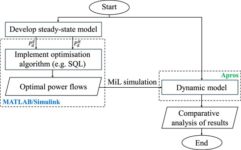
Figure 1. Flowchart of dynamic verification methodology for IESs.

Relevant details of the previous steps are discussed next.

2.1 Steady-state model

For this paper, the ‘energy hub’ modelling methodology was adopted (Eladl et al., 2023). The energy hub concept, introduced in (Geidl and Andersson, 2007b), provides a framework for steady-state modelling and simulation of IESs. Essentially, an energy hub links different energy vectors (e.g., heat, gas, electricity, hydrogen) via coupling technologies.

Figure 2 shows an example of an energy hub. The hub receives electricity and natural gas from their respective distribution networks as inputs, converts them to other energy forms, and stores them using different components such as a combined heat and power (CHP) unit, a gas boiler, an electric battery, and a thermal energy storage (TES) unit. These energy conversion and storage components, when operated in a coordinated manner, help fulfil the system’s energy demand—for example, for the system in Figure 2, electricity demand and heat demand. The operation of these elements within the energy hub could be optimised to minimise, for instance, operational costs, among other objective functions (see Section 2.2).

Figure 2

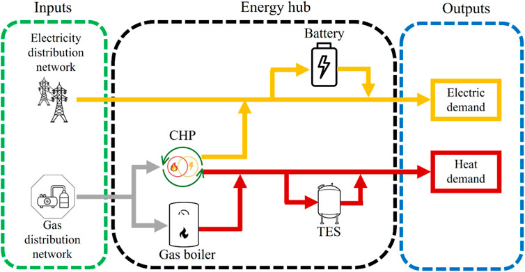
Figure 2. Example of an energy hub coupling electricity, gas, and heat. The energy hub considers two coupling technologies (a CHP unit and a gas boiler) and two energy storage devices (an electric battery and a TES unit).

Energy hub’s components establish redundant connections within the IES, offering two key benefits. Firstly, they enhance supply reliability for the loads, reducing dependence on a single network. Secondly, the additional flexibility enables optimal supply management by evaluating energy vector utilisation based on criteria such as cost, carbon emissions, and availability, ensuring the efficient utilisation of resources (Geidl et al., 2007).

The modelling concept of an energy hub enables analysing power flows through converter devices by determining their energy efficiency, which is calculated as the steady-state output and input ratio. When there are multiple energy vectors as inputs and outputs, a conversion matrix may be employed to mathematically establish connections between energy networks (Geidl et al., 2007).

2.2 Optimisation algorithm and optimisation module

Once a steady-state model of the system under investigation has been developed, as discussed in Section 2.1, an optimisation module is employed to meet operational specifications, such as minimising system operational costs and carbon emissions. The optimisation module requires the definition of an objective function subjected to a number of equality and inequality constraints (Frangopoulos, 2009). These constraints may depend on the characteristics of the system under study.

For an IES linking electricity, heat, and gas energy vectors as in the system shown in Figure 2, electrical and heat demand profiles are used as inputs to the optimisation module. The outputs of the module provide the optimal power flows for the system under study—thereby driving power dispatch and optimising system operation on a 24-h basis.

The optimisation approach here adopted differs from conventional multi-objective optimisation algorithms by employing a single-objective function that minimises operational and carbon emission costs simultaneously (Capone et al., 2021). The implementation is done in MATLAB 2021b, utilising the “fmincon” function (MathWorks, 2024), which employs the SQP algorithm. This algorithm is considered highly effective for non-linear programming and is characterised by a rapid convergence to optimal solutions (Bonnans et al., 2006; Nocedal and Wright, 2006).

The optimisation approach has been borrowed from (Morales Sandoval et al., 2023). To prevent duplication of published work, interested readers are referred to the reference for full details.

2.3 Dynamic model

The dynamic models used for components within a thermal-hydraulic system are based on differential equations that capture the transport phenomena of a heat transfer fluid (HTF), which is essentially a fluid employed to move thermal energy across two locations (Incropera et al., 2011). These equations include both the hydraulic characteristics, which detail the fluid flow, and the thermal attributes, which describe the temperature propagation. Valves, pipes, heat exchangers, hydraulic pumps, hydraulic separators, and energy storage tanks are typical elements considered in these models (De la Cruz-Loredo et al., 2022b).

In general, for an IES integrating heat as an energy vector, a dynamic model of the heating system is utilised to capture the slow thermal transients, which are often overlooked in traditional optimisation modules (Martinez Cesena et al., 2020).

2.3.1 Hydraulic components

The application of the Reynolds transport theorem, expressed for linear momentum, establishes the dynamic representation of a hydraulic component in a general way. This formulation assumes the characteristics of a one-dimensional flow and homogeneous incompressible fluid conditions (Cengel and Cimbala, 2010). Mathematically, this is given as

$\sum \overrightarrow{F}=V\frac{d}{dt}\left(\rho \overrightarrow{v}\right)=\rho V\frac{d\overrightarrow{v}}{dt}(1)$

In Eq. 1, $\rho$ [kg/m³] is the density of the fluid, $d\overrightarrow{v}/dt$ [m/s²] the rate of change of the linear velocity of the fluid, and $\sum \overrightarrow{F}$ [N] the summation of all the external forces acting on the volume $V$ [m³] of the hydraulic component. $\sum \overrightarrow{F}$ is expressed by the product of the flow area $A_f$ [m²] and the pressure differential $\Delta p_c$ [Pa] across the component as $\sum \overrightarrow{F}=A_f\Delta p_c$. For each hydraulic component, $\Delta p_c$ is given by (de la Cruz Loredo et al., 2022b):

$\Delta p_c=\frac{1}{2}\rho \left({\overrightarrow{v}}_0^2-{\overrightarrow{v}}^2\right)+\rho g\left(z_0-z\right)+\Delta p_f+\Delta p_L+\Delta p_B(2)$

where the first two terms in Eq. 2, $\frac{1}{2}\rho \left({\overrightarrow{v}}_0^2-{\overrightarrow{v}}^2\right)+\rho g\left(z_0-z\right)$, represent the pressure loss due to the hydrostatic and dynamic pressure differentials across the component, $g$ [m/s²] is the gravitational constant, $z_0$ and $z$ [m] are the heights of the inlet and outlet ports of the component, and ${\overrightarrow{v}}_0$ [m/s] the velocity of the fluid at the inlet port of the component. Also in the equation, $\Delta p_f$ is the pressure loss due to the fluid’s friction against the component’s internal walls, $\Delta p_L$ [Pa] is the pressure loss due to sudden changes in the flow path within the component, and $\Delta p_B$ [Pa] is the pressure boost generated by the component.

2.3.2 Thermal components

The dynamic model of a one-dimensional thermal component with a volume $V$ [m³] and containing an incompressible single phase HTF is given by (Incropera et al., 2011):

${\dot{H}}_C=\rho V{c}_{p,C}{\dot{T}}_C=\dot{m}\left(c_{p,in}{T}_{in}-c_{p,C}{T}_C\right)+\sum {\dot{Q}}_{conv}+\sum {\dot{Q}}_{cond}(3)$

where ${\dot{H}}_C$ [W] is the rate of change in the enthalpy of the fluid contained in the component, ${\dot{T}}_C$ [°C/s] is the rate of change in the temperature of the fluid, and $\rho$ [kg/m³] and $c_{p,C}$ [J/kg°C] are the density and specific heat value of the fluid at a temperature $T_C$ [°C]. The term $\dot{m}\left(c_{p,in}{T}_{in}-c_{p,C}{T}_C\right)$ is the rate of change in the components’ enthalpy owing to the mass exchange with other thermal components. The rate of mass flow exchange, or mass flow rate, is given by $\dot{m}$ [kg/s], where $T_{in}$ [°C] is the temperature of the fluid entering the component and $c_{p,in}$ [J/kg°C] the specific heat value of the fluid at $T_{in}$. $\sum {\dot{Q}}_{conv}$ and $\sum {\dot{Q}}_{cond}$ [W] are the summation of the different convection and conduction heat transfer events between the component and its surroundings.

Eq. 3 does not consider radiation heat transfer due to the negligible contribution of radiation within the temperature and environmental conditions considered in this paper. If radiation heat transfer effects had a representative contribution, an additional term would be required at the right-hand side of the equation (i.e., $\sum {\dot{Q}}_{rad}$).

2.4 Quantification method

By comparing the outcomes of the optimisation module (described in Section 2.2) with those of the dynamic model (Section 2.3), potential deviations in power flows and operational costs are quantified. This method allows assessing the impact of slow thermal dynamics on system performance, thereby providing stakeholders and system operators with valuable insights for decision-making. This step is described in further detail in Section 3.5 for the system under study, where the operational costs for two seasons of a calendar year are investigated.

3 Case study

3.1 System description

The system under study operates based on the electricity and heat consumption of QEH. The facility is connected to both an electricity network and a gas supply network and is structured into heating zones (HZs). Each heating zone is treated as an independent heat consumption unit within the primary heating system.

The architecture of the primary heating system involves 1,200 m of pipelines connecting seven HZs through main and boiler pipeline loops, as shown in Figure 3A. The boiler loop incorporates two CHP units with an output power of 1,400 kW and four GBs with an output power of 5,200 kW located in HZs 1, 2, 4, and 5 to meet electricity and heat demand (see Figure 3B).

Figure 3

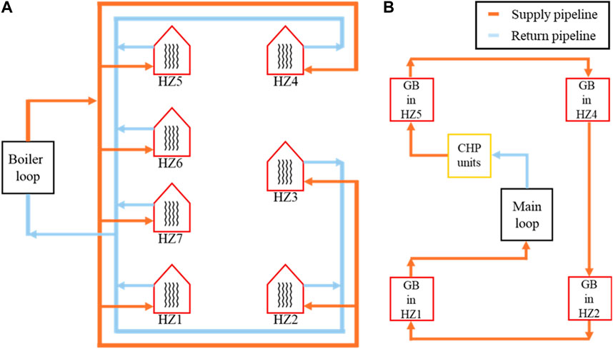
Figure 3. (A) Schematic of the primary heating system of QEH. (B) Boiler loop structure of the heating system of QEH (De la Cruz-Loredo et al., 2022b).

The original system configuration shown in Figure 3 was modified to incorporate sustainable energy technologies, in line with UK’s National Health Service and national targets to reduce greenhouse gas emissions (NHS Foundation Trust, 2015).

The upgraded IES is shown in Figure 4. This system configuration includes the two CHP units, 3 GBs located in HZs 1, 2, and 4, and an electric boiler (EB) in HZ5 within the boiler loop. In addition, a 100 m³ TES system consisting of four interconnected hot water tanks was considered. This sensible heat TES system is connected at the bottom to the return pipeline of the main loop and at the top to the boiler loop, after the GB in HZ1, for charging purposes. To avoid any disturbance to the supply temperature in the boiler loop, the TES system discharges immediately before the GB in HZ1 (De la Cruz-Loredo et al., 2022b).

Figure 4

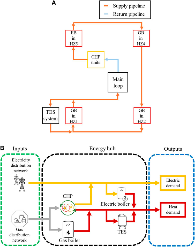
Figure 4. (A) Boiler loop structure of the upgraded dynamic model implemented in Apros (De la Cruz-Loredo et al., 2022b). (B) Steady-state schematic for the upgraded IES optimisation.

In both the optimisation module and the dynamic model utilised for this study, the two individual CHP units within the physical system are considered as a single CHP unit with an equivalent output power for simplicity. Therefore, reference to the CHP units will be made using the term “CHP plant” to denote the collective operation of the units as a single entity.

Table 1 shows the considered capacities of the retrofitted technologies. These have been selected based on practical specifications and availability in the UK market (London Engineers Company, 2023; Refrigeration Technology Co. Ltd, 2023). For the different system configurations studied in this paper, the schematics and essential mathematical formulations for each are outlined in Supplementary Appendix SA.

Table 1

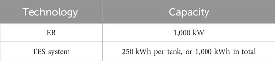
Table 1. Capacities of the incorporated technologies.

3.2 System modelling for optimisation

Real electricity and heat demand profiles from QEH were used as inputs to the optimisation module. These profiles correspond to different seasons of the year and are provided in Supplementary Appendix SB. However, to maintain control over supply and return temperatures and prevent fluctuations in the dynamic model, an overestimation of electrical demand and underestimation of heat demand were considered. A 1-h granularity was employed.

Figure 5 shows the daily price profiles for gas and electricity adopted in this paper based on energy prices available at the hospital site in 2020 and average market prices (Guelpa, 2024).

Figure 5

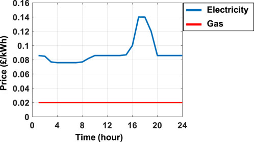
Figure 5. Hourly gas and electricity prices.

The following assumptions were considered for system modelling within the optimisation module (based on the data provided by QEH and information available in the literature) (Morales Sandoval et al., 2023):

i. The system is considered to be in steady-state between any two time periods.

ii. There are no stand-by energy losses from system components.

iii. The gas-to-electricity conversion efficiency (${\eta }_{CHP}^{g/e}$) of the CHP plant is 37.8% and its gas-to-heat conversion efficiency (${\eta }_{CHP}^{g/h}$) is 49.7%.

iv. The efficiency of the GB (${\eta }_{GB}$) is 81% (Brumbaugh, 2004).

v. The efficiency of the EB (${\eta }_{EB}$) is 100% (de la Cruz Loredo et al., 2022a).

vi. The charging and discharging efficiencies of the TES system (${\eta }_{TES}$) are 90% (Geidl and Andersson, 2007b).

vii. Exporting surplus electricity from the IES back to the external grid is not provisioned in this case study.

3.3 Dynamic modelling for the system under study

A detailed dynamic model of the heating system was implemented. However, representation of the electricity system, for simplicity, was limited to reproduce the energy balance between supply and demand based on real historical data. The dynamic model was implemented in Apros using available library models (de la Cruz Loredo et al., 2022a; 2022b).

The following modelling assumptions were considered:

i. A constant pressure loss coefficient $K_L=0.1$ was adopted for all components.

ii. All components in the heating system are covered with a 40 mm thick insulating layer with a constant conduction heat transfer coefficient value of $\kappa =0.025$ W/(m°C).

iii. Heat supply and demand were implemented as single external heat flows generating or consuming heat from a pipeline element.

iv. As for system optimisation (see Section 3.2), exporting surplus electricity from the IES back to the external grid is not provisioned.

The operation of the hospital’s heating system was regulated by a process control system consisting of four control elements: the marginal differential pressure control, the supply temperature control, the return temperature control, and the TES system control. These elements regulate pressure, flow, and temperature within different sections of the IES by adjusting parameters such as pump speed, valve opening range, and heat flow from the heat generation units. For this purpose, proportional-integral (PI) controllers were employed. Table 2 shows relevant specifications of these controllers.

Table 2

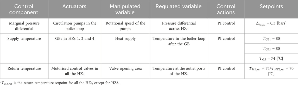
Table 2. Specifications of the marginal pressure differential, supply and return temperatures controllers (de la Cruz Loredo et al., 2022a).

Similar to the optimisation module, real electricity and heat demand profiles from QEH were used. As mentioned before, these are provided in Supplementary Appendix SB. However, the dynamic model adopted a 30-min granularity for the energy demand data.

3.4 Optimisation module

The energy system needs to select the optimal proportion of electricity and gas intake to reduce energy costs and the production of CO₂. To minimise the daily operational cost of the system while also minimising carbon emissions, the objective function is expressed as (Morales Sandoval et al., 2023)

$C={\displaystyle \sum _{i=1}^{24}}\left[\left(C_{grid,i}^E\times P_{grid,i}^E\right)+\left(C_{grid,i}^G\times P_{grid,i}^G\right)+\left(C_{{CO}_2}^E\right)+\left(C_{{CO}_2}^G\right)\right](4)$

where $C$ is the daily operational cost, $C_{grid,i}^E$ and $C_{grid,i}^G$ are the electricity and gas unit costs at hour i, $P_{grid,i}^E$ and $P_{grid,i}^G$ are the power inputs to the energy system from the external electricity and gas networks at hour i, and $C_{{CO}_2}^E$ and $C_{{CO}_2}^G$ are the costs of CO₂ production associated with electricity and gas consumption.

Objective function in Eq. 4 is subject to the following equality constraints (representing the electricity and heat balance equations)

$P_{grid,i}^E+{\eta }_{CHP}^{g/e}{P}_{CHP,i}^G-{\eta }_{EB}{P}_{EB,i}=P_{d,i}^{E}i=1,2,3,\dots 24(5)$

${\eta }_{CHP}^{g/h}{P}_{CHP,i}^G+{\eta }_{GB}{P}_{GB,i}^G+{\eta }_{EB}{P}_{EB,i}-P_{ch,i}^{TES}+P_{dis,i}^{TES}=P_{d,i}^{H}i=1,2,3,\dots 24(6)$

where $P_{CHP,i}^G$ and $P_{GB,i}^G$ are the power inputs to the CHP plant and the GBs from the gas grid; $P_{EB,i}$ is the electrical power input to the EB either from the electric grid or from the surplus produced by the CHP plant; and $P_{ch,i}^{TES}$ and $P_{dis,i}^{TES}$ represent the charging and discharging powers of the TES system.

Based on the dimensions of hot water tanks available in the market and considering the supply and return temperatures of the IES under study (de la Cruz Loredo et al., 2022b; Refrigeration Technology Co. Ltd, 2023), the capacity of the TES system used in this paper was selected as 1,000 kWh (Majić et al., 2013) (250 kWh per individual hot water tank, see Table 1). Its charging and discharging powers $P_{ch,i}^{TES}$ and $P_{dis,i}^{TES}$ per time period (i.e. 1 h) are constrained as

$0\le P_{ch,i}^{TES}\le 250\left(\text{kW}\right)(7)$

$0\le P_{dis,i}^{TES}\le 250\left(\text{kW}\right)(8)$

To ensure the energy levels in the thermal store remain within the predefined maximum and minimum limits, the following constraints were imposed:

${\displaystyle \sum _{i=1}^j}\left[{\eta }_{TES}{P}_{ch,i}^{TES}-1/{\eta }_{TES}{P}_{dis,i}^{TES}\right]\times ∆t\le L_{\mathit{max}}^{TES}j=1,2,3,\dots 24(9)$

${\displaystyle \sum _{i=1}^j}\left[{\eta }_{TES}{P}_{ch,i}^{TES}-1/{\eta }_{TES}{P}_{dis,i}^{TES}\right]\times ∆t\ge L_{\mathit{min}}^{TES}j=1,2,3,\dots 24(10)$

where $∆t$ is the hourly time period considered in the optimisation algorithm, and $L_{\mathit{max}}^{TES}$ and $L_{\mathit{min}}^{TES}$ are the maximum and minimum capacities of the TES system.

In the previous formulation, Eqs 5, 6 denote the equality constraints, while Eqs 7-10 denote inequality constraints to meet the objective function in Eq. 4.

To ensure the energy stored in the TES system at the end of the diurnal cycle remains the same as during the start of the cycle, the following equality constraint was included:

${\displaystyle \sum _{i=1}^{24}}{P}_{ch,i}^{TES}-P_{dis,i}^{TES}=0(11)$

Constraint in Eq. 11 enables the cyclic operation of the energy storage unit.

3.5 Quantification of operational costs

To assess operational costs, two contrasting seasons, summer and winter, were selected to represent periods of high and low heat demand across the year. For simplicity and to provide a basis for discussion, weekly costs were extrapolated to account for 52 weeks in a year. This way, the annual operating cost for each scenario under investigation was determined using

$C_a=\left(C_w^S\times 26\right)+\left(C_w^W\times 26\right)(12)$

where $C_a$ is the estimated annual cost of the IES and $C_w^S$ and $C_w^W$ represent the weekly operational cost for summer and winter.

3.6 Implementation

Different software packages may be adopted for simulating the complex dynamics of real IESs, facilitating the adoption of a model-based design approach. This approach enables the development of dynamic models, control, and communication systems to conduct virtual tests—eliminating the need for costly verification in real systems. Following this approach, the effectiveness of the optimisation algorithm was demonstrated through an MiL configuration.

MiL simulation was carried out as a co-simulation utilising two software platforms, as shown in Figure 6. The optimisation algorithm and dynamic models of the CHP plant and the EB were implemented in MATLAB/Simulink, while the control schemes and dynamic models of the TES system and the heating network were developed in Apros. The connection between the two software platforms was achieved through the utilisation of an open platform communications (OPC) protocol, which is available in both MATLAB and Apros (OPC foundation, 2024). Such a co-simulation architecture has been successfully adopted in the literature (Morales Sandoval et al., 2021; de la Cruz Loredo et al., 2022a, 2022b; Bastida et al., 2023).

Figure 6

Figure 6. Co-simulation framework for the dynamic verification.

3.7 Scenarios

Three different system configurations—namely, Scenario 1 (base case, see Supplementary Figure SA1), Scenario 2 (IES with a TES system, Supplementary Figure SA2), and Scenario 3 (IES with EB and a TES system Supplementary Figure SA3)—were chosen to quantify discrepancies in power flows and operational cost by comparing the outcomes of the optimisation module and the dynamic model.

4 Results

To evaluate the performance of the optimisation module against that of the dynamic model, the three systems defined in Section 3.7 were considered.

As discussed in Section 3.5, the operational costs for each IES configuration was determined by extrapolating weekly costs using Eqs 4, 12. A summary of the results is presented in Table 3; where significant differences between the operational cost for the three defined systems are observed. The operational costs obtained by the dynamic model compared to those by the optimisation module are higher by 5.5% for the base case (Scenario 1), by 5.3% for the system upgraded with a TES system (Scenario 2), and by 5.4% for an upgraded system with an EB and a TES system (Scenario 3). The higher costs exhibited by the dynamic simulations could be attributed to the consideration of real-world complexities, such as losses, non-linearity, transient phenomena in different system components, and differences between demand forecasts and actual demand—which are neglected in optimisation studies.

Table 3

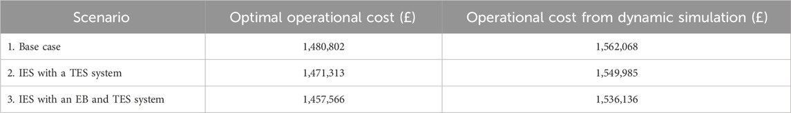
Table 3. Summary of annual operational costs for different IES scenarios.

A detailed discussion for each system configuration is presented next to delve further into the comparative analysis. For the sake of visualisation and simplicity of the explanation, the analysis is focussed on the first day of the week for each scenario, with operational costs quantified for the full week. For further details on the weekly comparison, interested readers are directed to Supplementary Appendix SC, which provides additional graphical results covering the entire week under study.

4.1 Scenario 1

The base case, similar to the current system configuration at QEH, is examined in more detail in this section. In this case, the electricity and heat demand are met through the external electricity grid, CHP plant and GBs. Figure 7 compares the optimal heat power output ${\dot{Q}}_{CHP,opt}$ produced by the CHP plant during a day in summer (see Figure 7A, green trace) and winter (Figure 7B, blue trace) with the heat power output ${\dot{Q}}_{CHP,dyn}$ obtained with the dynamic model (orange and purple traces in the figures, with markers). Given that operation of the CHP plant is dictated by the optimisation module and the electricity demand fluctuations being balanced with the electricity grid, a good agreement is observed in heat power flows. In response to the higher energy demand during winter, an increase in the use of the CHP plant can be noticed in both cases.

Figure 7

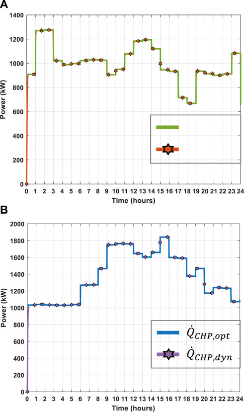
Figure 7. Scenario 1. Comparison of heat power flows for CHP plant. Day in: (A) summer and (B) winter.

Figure 8 shows a comparison between the heat power flows ${\dot{Q}}_{GBs,opt}$ of GBs for a summer day (Figure 8A, green trace) and a winter day (Figure 8B, blue trace) obtained with the optimisation module and via dynamic simulation (${\dot{Q}}_{GBs,dyn}$, orange and purple traces). Here, the differences in heat power flows become evident with higher energy demand in winter, leading to a significant increase in the utilisation of GBs. While the dynamic model aims to replicate the optimal heat power flows, the influence of system dynamics is evident in the model output. Therefore, in scenarios involving large quantities of heat flows (e.g., in winter months with higher heat demand), the discrepancy between the static optimisation module and the dynamic system model becomes more pronounced.

Figure 8

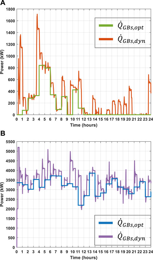
Figure 8. Scenario 1. Comparison of heat power flows for GBs. Day in: (A) summer and (B) winter.

The heat power flow variations exhibited by GBs have an impact on the estimation of daily and weekly operational costs in summer and winter. The weekly operational costs are shown in Table 4. During the week in summer, the operational cost resulting from the dynamic model deviates by £836.28 (equivalent to 4.87%) from the estimated optimal operational cost. In the winter week, with the increased GBs usage, a notable deviation in operational cost is observed, where the output of the dynamic model differs from that of the optimal model by £2289.34, or 5.75%.

Table 4

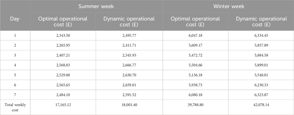
Table 4. Operational costs of the base case obtained from optimisation and dynamic simulations.

4.2 Scenario 2

In Scenario 2, the electricity and heat demand are met through the external electricity grid, CHP plant, GBs, and TES system. Figure 9 compares the optimal heat power output ${\dot{Q}}_{CHP,opt}$ produced by the CHP plant during a day in summer (Figure 9A, green trace) and winter (Figure 9B, blue trace) with that obtained with the dynamic model (${\dot{Q}}_{CHP,dyn}$, orange and purple traces with markers).

Figure 9

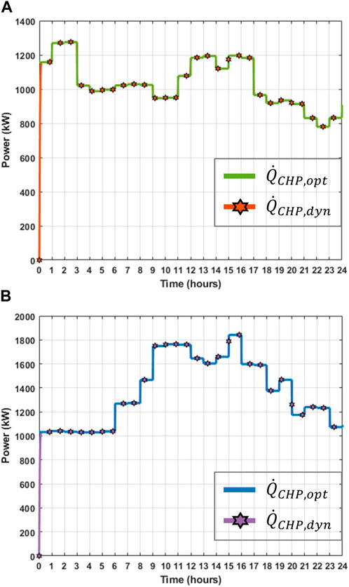
Figure 9. Scenario 2. Comparison of heat power flows for CHP plant. Day in: (A) summer and (B) winter.

Comparing Figure 9A with Figure 7A from Scenario 1, it can be observed that both the optimal power output produced by the CHP plant (${\dot{Q}}_{CHP,opt}$, green traces in both figures) and the heat power output obtained with the dynamic model (${\dot{Q}}_{CHP,dyn}$, orange traces with markers in both figures) vary during the summer day when a TES system is present in the system. This variation is influenced by energy demand and cost. For instance, during hours 15 to 19, electricity demand is high while heat demand is low (refer to Supplementary Figure SB1). Consequently, surplus heat from the CHP plant is directed to the TES system. This stored heat can be utilised during periods of increased energy cost, resulting in operational cost savings. The heat power output produced by the CHP plant during the winter day is similar as in the base case considered as Scenario 1 (Figures 7B, 9B, see all traces in the figures). This is because the incorporation of a TES system into the IES does not have any effect in the winter season as it is not operative.

Figure 10 shows a comparison between the heat power flows ${\dot{Q}}_{GBs,opt}$ of GBs for a day in summer (Figure 10A, green trace) and winter (Figure 10B, blue trace) obtained with the optimisation module and dynamic simulation (${\dot{Q}}_{GBs,dyn}$, orange and purple traces). A decrease in the heat power output produced by the GBs during summer is noticed when compared to Scenario 1 (comparing Figure 10A with Figure 8A, green traces in both figures). For instance, here the maximum peak of the optimal heat power output produced by the GBs is around 700 kW, against the peak of approximately 850 kW observed in Scenario 1 (Figure 8A). However, it is important to note that the heat power output produced by GBs in the winter day for Scenario 2 remains unchanged compared to that of Scenario 1 (see all traces in Figures 8B, 10B).

Figure 10

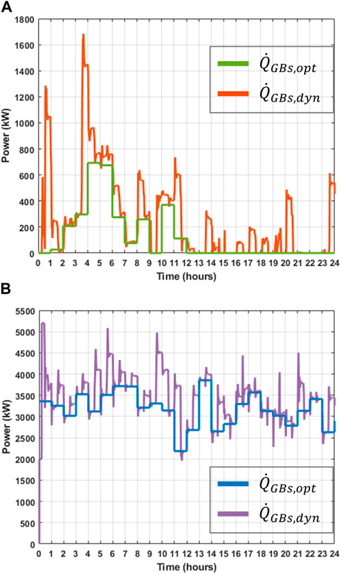
Figure 10. Scenario 2. Comparison of heat power flows for GBs. Day in: (A) summer and (B) winter.

Figure 11 compares the performance of the TES system during both summer (Figure 11A) and winter (Figure 11B) days. In Figure 11A, negative values indicate the TES system is charging, while positive values mean the TES system is discharging. A clear discrepancy is observed between the optimal performance indicated by the optimisation module (${\dot{Q}}_{TES,opt}$, green trace) and the dynamic performance achieved by the dynamic simulation (${\dot{Q}}_{TES,dyn}$, orange trace with markers) during the day in summer. Figure 11B confirms that the TES system is not operational during the winter day, with no charging or discharging occurring. This is consistent with the discussion around Figure 9B.

Figure 11

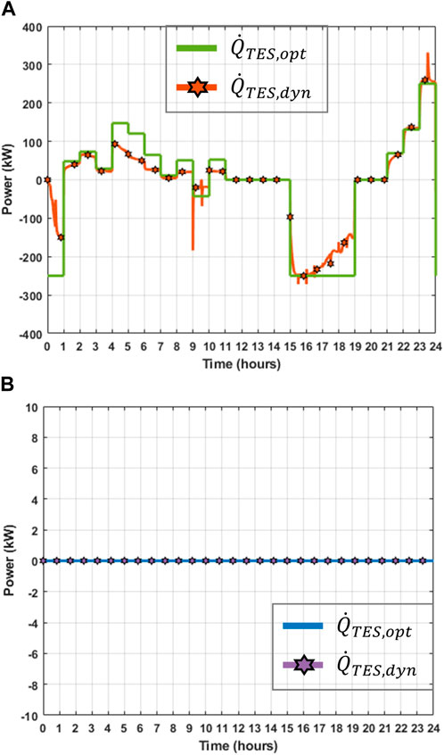
Figure 11. Scenario 2. Comparison of TES system performance. Day in: (A) summer and (B) winter.

The variations in heat power flow exhibited for Scenario 2 affect the estimation of daily and weekly operational costs in both summer and winter, as detailed in Table 5. During the summer week, the operational cost resulting from the dynamic model deviates by £736.7 (equivalent to 4.38%) from the estimated optimal operational cost. In the winter week, a deviation of 5.75% exists between the output of the dynamic model and that of the optimisation module, as the TES system remains idle—consistent with results obtained in Scenario 1.

Table 5

Table 5. Operational costs of the IES with TES system obtained from optimisation and dynamic simulations.

4.3 Scenario 3

For Scenario 3, electricity and heat demand are met through the external electricity grid, CHP plant, GBs, EB, and TES system. Figure 12 compares the optimal heat power output ${\dot{Q}}_{CHP,opt}$ produced by the CHP plant during the day in summer (Figure 12A, green trace) and winter (Figure 12B, blue trace) with those obtained with the dynamic model (${\dot{Q}}_{CHP,dyn}$, orange and purple traces with markers). An increase in the heat output power provided by the CHP plant during the summer day (Figure 12A) compared to both Scenario 1 (see Figure 7A) and Scenario 2 (Figure 9A) is observed in the initial hours of the day by both the optimisation module and the dynamic simulation. This increase is attributed to the surplus electricity generated by the CHP plant being utilised to power the EB, which entirely converts the electricity consumed to heat supply due to its high efficiency. The same behaviour occurs in the winter day (Figure 12B), where the CHP plant operates at maximum capacity to generate surplus electricity while meeting the heat demand.

Figure 12

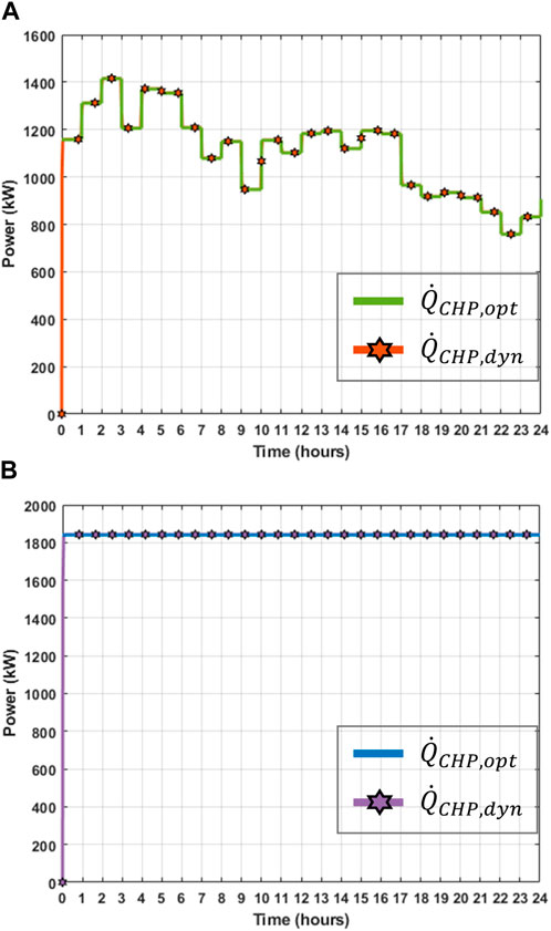
Figure 12. Scenario 3. Comparison of heat power flows for CHP plant. Day in: (A) summer and (B) winter.

Figure 13 shows a comparison between the heat power flows ${\dot{Q}}_{GBs,opt}$ of GBs for the summer (Figure 13A) and winter (Figure 13B) days obtained with the optimisation module (green and blue traces) and dynamic simulation (${\dot{Q}}_{GBs,dyn}$, orange and purple traces). During the summer day (Figure 13A), the optimisation module does not operate the GBs (see green trace, with values of zero throughout) as the heat demand is met with the EB. However, the dynamic model requires GBs to regulate the supply temperature within the system and prevent disturbances in temperature, as illustrated by the orange trace. During the winter day (Figure 13B), a reduction in the utilisation of the GBs is observed compared to Scenario 1 (Figure 8B) and Scenario 2 (Figure 10A). This decrease is due to the support provided by the EB in meeting the heat demand.

Figure 13

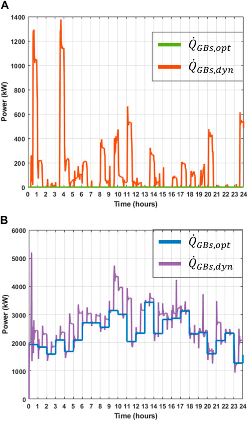
Figure 13. Scenario 3. Comparison of heat power flows for GBs. Day in: (A) summer and (B) winter.

Similar to the management of the CHP plant, the operation of the EB is governed by the optimisation module for power dispatch. As a result, the discrepancies between the optimal heat power output (${\dot{Q}}_{EB,dyn}$) and that obtained with the dynamic model (${\dot{Q}}_{EB,dyn}$) are minimal, as shown in Figure 14.

Figure 14

Figure 14. Scenario 3. Comparison of heat power flows for EB. Day in: (A) summer and (B) winter.

Figure 15 compares the optimal and dynamic performance of the TES system during both summer (Figure 15A) and winter (Figure 15B) days. As in Scenario 2, a discrepancy is observed between the optimal behaviour suggested by the optimisation module (${\dot{Q}}_{TES,opt}$) and the dynamic performance achieved via simulations (${\dot{Q}}_{TES,dyn}$) during the summer day. As before, the TES system remains idle during the winter day (see Figure 15B).

Figure 15

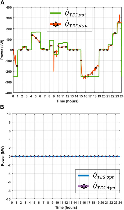
Figure 15. Comparison of TES system performance. Day in: (A) summer and (B) winter.

Table 6 compares the weekly operational costs for Scenario 3. During the summer week, the operational cost resulting from the dynamic simulations deviates by £731.58 (equivalent to 4.36%) from the estimated optimal operational cost. In the winter week, the operational cost obtained with dynamic simulations differs from that of the optimal model by £2290.37, or 5.83%.

Table 6

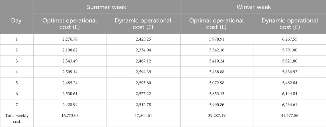
Table 6. Operational costs of the IES with an EB and TES system obtained from optimisation and dynamic simulations.

5 Conclusion

A methodology enabling the dynamic verification of an optimisation algorithm for the power dispatch of IESs was presented in this paper. The algorithm assumed steady-state operation of the IES components between consecutive time-steps, while minimising operating cost and emissions. A dynamic model of the IES was adopted in tandem to account for the real-word physical phenomena, such as the transient response of thermal systems and non-linearity of system components, which were not considered in the steady-state optimisation module. The two models were then compared by using a series of scenarios and real data from a civic building in the UK dedicated to health services. The scenarios considered the base system upgraded with low-carbon technologies to reflect national targets to reduce carbon emissions.

The optimisation module and the dynamic model were integrated through an MiL co-simulation approach, where MATLAB/Simulink was interfaced with Apros using the OPC protocol. This approach enabled an assessment of the discrepancies between the steady-state optimisation and the dynamic model, providing valuable insights into the practical implications of real-time operation of the IES under study.

The key findings, implications, and recommendations arising from this research work are outlined next:

• The optimisation and dynamic simulations yielded different power flows for system components, with significant discrepancies for GBs and smaller differences for the CHP plant. Both approaches suggested the use of the TES system only in summer months, where the relative availability of thermal energy was greater compared to its demand. Furthermore, both models suggested a higher degree of utilisation of the EB in winter and showed more disparity in the estimated power flows in summer.

• The discrepancies in power flows led to higher operational costs in dynamic simulations compared to optimal solutions. This highlights the potential limitations of traditional optimisation algorithms and underpins the recommendation to consider real-world complexities associated with the IES, such as losses, non-linear behaviour of components, and transient phenomena while optimising IESs.

• The TES system increased the flexibility of the IES, allowing surplus heat to be stored during off-peak periods for later use during peak heating demand periods, resulting in operational cost savings. Incorporating an EB into the IES created opportunities to utilise surplus electricity generated by the CHP plant for highly efficient conversion to heat, reducing conventional heat generation.

• The approach provided by the presented methodology may be useful for energy management and planning by decision-makers to understand the practical implications of real-time operation of an IES and how these may affect operational costs.

Data availability statement

The datasets presented in this article are not readily available because raw data is owned by a third party. Requests to access the datasets should be directed to Ugalde-LooC@cardiff.ac.uk.

Author contributions

DM: Data curation, Formal Analysis, Investigation, Methodology, Software, Validation, Visualization, Writing–original draft, Writing–review and editing. ID: Conceptualization, Formal Analysis, Investigation, Methodology, Software, Validation, Writing–review and editing. PS: Methodology, Resources, Supervision, Writing–review and editing. MA: Resources, Supervision, Writing–review and editing. CU-L: Conceptualization, Funding acquisition, Methodology, Project administration, Resources, Supervision, Writing–original draft, Writing–review and editing.

Funding

The author(s) declare that financial support was received for the research, authorship, and/or publication of this article. The work presented in this paper was supported by the Engineering and Physical Sciences Research Council (EPSRC), UK Research and Innovation, through the projects “Flexibility from Cooling and Storage (Flex-Cool-Store)” under grant EP/V042505/1, and “Multi-energy Control of Cyber-Physical Urban Energy Systems (MC2)” under grant EP/T021969/1.

Acknowledgments

The authors acknowledge the support and contribution from the estates office at Queen Elizabeth Hospital for providing data and energy system information for this paper.

Conflict of interest

The authors declare that the research was conducted in the absence of any commercial or financial relationships that could be construed as a potential conflict of interest.

Publisher’s note

All claims expressed in this article are solely those of the authors and do not necessarily represent those of their affiliated organizations, or those of the publisher, the editors and the reviewers. Any product that may be evaluated in this article, or claim that may be made by its manufacturer, is not guaranteed or endorsed by the publisher.

Supplementary material

The Supplementary Material for this article can be found online at: https://www.frontiersin.org/articles/10.3389/fenrg.2024.1385839/full#supplementary-material

References

Alper, A., and Oguz, O. (2016). The role of renewable energy consumption in economic growth: evidence from asymmetric causality. Renew. Sustain. Energy Rev. 60, 953–959. doi:10.1016/j.rser.2016.01.123

CrossRef Full Text | Google Scholar

Bastida, H., De la Cruz-Loredo, I., and Ugalde-Loo, C. E. (2023). Effective estimation of the state-of-charge of latent heat thermal energy storage for heating and cooling systems using non-linear state observers. Appl. Energy 331, 120448. doi:10.1016/j.apenergy.2022.120448

CrossRef Full Text | Google Scholar

Bonnans, J., Gilbert, J., Lemaréchal, C., and Sagastizábal, C. (2006) Numerical optimization: theoretical and practical aspects. Springer Science and Business Media.

Google Scholar

Brumbaugh, J. (2004). “Audel HVAC fundamentals,” in Heating systems, furnaces and boilers (John Wiley and Sons).

Google Scholar

Capone, M., Guelpa, E., and Verda, V. (2021). Multi-objective optimization of district energy systems with demand response. Energy 227, 120472. doi:10.1016/j.energy.2021.120472

CrossRef Full Text | Google Scholar

Cengel, Y., and Cimbala, J. (2010) Fluid mechanics: fundamentals and applications. 1st ed. New York: McGraw-Hill Higher Education.

Google Scholar

Chen, H., Li, D., Wang, S., Zhong, M., Liu, K., Jia, X., et al. (2022) “Optimization strategy verification of integrated energy system operation based on dynamic simulation,” in 2022 IEEE 6th conference on energy internet and energy system integration, 1223–1228. doi:10.1109/EI256261.2022.10117153

CrossRef Full Text | Google Scholar

Chesi, A., Ferrara, G., Ferrari, L., Magnani, S., and Tarani, F. (2013). Influence of the heat storage size on the plant performance in a Smart User case study. Appl. Energy 112, 1454–1465. doi:10.1016/j.apenergy.2013.01.089

CrossRef Full Text | Google Scholar

Climate Change Committee (2023). Net Zero: the UK’s contribution to stopping global warming. Available at: https://www.theccc.org.uk/publication/net-zero-the-uks-contribution-to-stopping-global-warming/ (Accessed August 02, 2023).

Google Scholar

De la Cruz-Loredo, I., Ugalde-Loo, C. E., and Abeysekera, M. (2022b). Dynamic simulation and control of the heat supply system of a civic building with thermal energy storage units. IET Generation, Transm. Distribution 16, 2864–2877. doi:10.1049/gtd2.12453

CrossRef Full Text | Google Scholar

De la Cruz Loredo, I., Ugalde-Loo, C. E., Abeysekera, M., Morales Sandoval, D. A., Bastida, H., and Zhou, Y. (2022a). Ancillary services provision from local thermal systems to the electrical power system. CIGRE Sess. 2022.

Google Scholar

Ding, L., Gao, J., Shi, G., and Ni, Z. (2022). Robust optimal dispatch of integrated energy system considering with coupled wind and hydrogen system. J. Phys. Conf. Ser. 2215, 012001. doi:10.1088/1742-6596/2215/1/012001

CrossRef Full Text | Google Scholar

Eladl, A. A., El-Afifi, M. I., El-Saadawi, M. M., and Sedhom, B. E. (2023). A review on energy hubs: models, methods, classification, applications, and future trends. Alexandria Eng. J. 68, 315–342. doi:10.1016/j.aej.2023.01.021

CrossRef Full Text | Google Scholar

European Scientific Advisory Board on Climate Change (2024). Scientific advice for the determination of an EU-wide 2040 climate target and a greenhouse gas budget for 2030-2050. Available at: https://climate-advisory-board.europa.eu/reports-and-publications/scientific-advice-for-the-determination-of-an-eu-wide-2040 (Accessed September 16, 2023).

Google Scholar

Fortum (2024). Apros nuclear - advanced process simulation software. Available at: https://www.fortum.com/services/nuclear/process-simulation-and-safety-analysis/apros (Accessed August 9, 2022).

Google Scholar

Frangopoulos, C. (2009) Exergy, energy system analysis and optimization volume II: thermoeconomic analysis modeling, simulation and optimization in energy systems. EOLSS Publications.

Google Scholar

Guelpa (2024). Gas and electricity prices in the non-domestic sector. Available at: https://www.gov.uk/government/statistical-data-sets/gas-and-electricity-prices-in-the-non-domesticsector/ (Accessed 2 February 2024).

Google Scholar

Geidl, M., and Andersson, G. (2007a). Optimal power flow of multiple energy carriers. IEEE Trans. Power Syst. 22, 145–155. doi:10.1109/TPWRS.2006.888988

CrossRef Full Text | Google Scholar

Geidl, M., and Andersson, G. (2007b). “Optimal coupling of energy infrastructures,” in 2007 IEEE lausanne power Tech (IEEE), 1398–1403. doi:10.1109/PCT.2007.4538520

CrossRef Full Text | Google Scholar

Geidl, M., Koeppel, G., Favre-Perrod, P., Klockl, B., Andersson, G., and Frohlich, K. (2007c). Energy hubs for the future. IEEE Power Energy Mag. 5, 24–30. doi:10.1109/MPAE.2007.264850

CrossRef Full Text | Google Scholar

Gielen, D., Boshell, F., Saygin, D., Bazilian, M. D., Wagner, N., and Gorini, R. (2019). The role of renewable energy in the global energy transformation. Energy Strategy Rev. 24, 38–50. doi:10.1016/j.esr.2019.01.006

CrossRef Full Text | Google Scholar

Gonzalez, I., Castello, P., Sgobbi, A., Nijs, W., Quoilin, S., Zucker, A., et al. (2015) Addressing flexibility in energy system models. Luxembourg.

Google Scholar

Good, N., Martínez Ceseña, E. A., and Mancarella, P. (2017). Ten questions concerning smart districts. Build. Environ. 118, 362–376. doi:10.1016/j.buildenv.2017.03.037

CrossRef Full Text | Google Scholar

Gov.uk (2024). Gas and electricity prices in the non-domestic sector. Available at: https://www.gov.uk/government/statistical-data-sets/gas-and-electricity-prices-in-the-non-domestic-sector (Accessed May 6, 2022).

Google Scholar

Guelpa, E., and Verda, V. (2019). Thermal energy storage in district heating and cooling systems: a review. Appl. Energy 252, 113474. doi:10.1016/j.apenergy.2019.113474

CrossRef Full Text | Google Scholar

Incropera, F., DeWitt, D. P., Bergman, T. L., and Lavine, A. S. (2011) Fundamentals of heat and mass transfer. 7th ed. Hoboken, NJ: John Wiley and Sons.

Google Scholar

International Energy Agency (IEA) (2024). World energy outlook 2020. Available at: https://www.iea.org/reports/world-energy-outlook-2020 (Accessed November 4, 2023).

Google Scholar

International Renewable Energy Agency (IRENA) (2024) Renewable energy policies in a time of transition heating and cooling. Available at: https://www.irena.org/publications/2020/Nov/Renewable-energy-policies-in-a-time-of-transition-Heating-and-cooling (Accessed October 9, 2023).

Google Scholar

Kim, M. J., Song, H.-Y., Park, J.-B., and Roh, J.-H. (2016). “Optimization of CHP and thermal storage under heat demand,” in 2016 12th IEEE international conference on control and automation (ICCA) (IEEE), 277–281. doi:10.1109/ICCA.2016.7505289

CrossRef Full Text | Google Scholar

London Engineers Company (2023). Lecompany; electric heating boilers. Available at: https://www.lecompany.co.uk/electric-heating-boilers.html (Accessed November 7, 2023).

Google Scholar

Majić, L., Krželj, I., and Delimar, M. (2013). “Optimal scheduling of a CHP system with energy storage,” in 36th international convention on information and communication Technology, electronics and microelectronics (Croatia: Opatija), 1253–1257.

Google Scholar

Martinez Cesena, E. A., Loukarakis, E., Good, N., and Mancarella, P. (2020). Integrated electricity– heat–gas systems: techno–economic modeling, optimization, and application to multienergy districts. Proc. IEEE 108, 1392–1410. doi:10.1109/JPROC.2020.2989382

CrossRef Full Text | Google Scholar

MathWorks (2024). Fmincon function documentation. Available at: https://uk.mathworks.com/help/optim/ug/fmincon.html (Accessed April 12, 2022).

Google Scholar

Mehregan, M., Abbasi, M., and Majid Hashemian, S. (2022). Technical, economic and environmental analyses of combined heat and power (CHP) system with hybrid prime mover and optimization using genetic algorithm. Sustain. Energy Technol. Assessments 49, 101697. doi:10.1016/j.seta.2021.101697

CrossRef Full Text | Google Scholar

Mitali, J., Dhinakaran, S., and Mohamad, A. A. (2022). Energy storage systems: a review. Energy Storage Sav. 1, 166–216. doi:10.1016/j.enss.2022.07.002

CrossRef Full Text | Google Scholar

Moeini-Aghtaie, M., Abbaspour, A., Fotuhi-Firuzabad, M., and Hajipour, E. (2014). A decomposed solution to multiple-energy carriers optimal power flow. IEEE Trans. Power Syst. 29, 707–716. doi:10.1109/TPWRS.2013.2283259

CrossRef Full Text | Google Scholar

Morales Sandoval, D. A., De La Cruz Loredo, I., Bastida, H., Badman, J. J. R., and Ugalde-Loo, C. E. (2021). Design and verification of an effective state-of-charge estimator for thermal energy storage. IET Smart Grid 4, 202–214. doi:10.1049/stg2.12024

CrossRef Full Text | Google Scholar

Morales Sandoval, D. A., Saikia, P., De la Cruz-Loredo, I., Zhou, Y., Ugalde-Loo, C. E., Bastida, H., et al. (2023). A framework for the assessment of optimal and cost-effective energy decarbonisation pathways of a UK-based healthcare facility. Appl. Energy 352, 121877. doi:10.1016/j.apenergy.2023.121877

CrossRef Full Text | Google Scholar

Nemati, M., Braun, M., and Tenbohlen, S. (2018). Optimization of unit commitment and economic dispatch in microgrids based on genetic algorithm and mixed integer linear programming. Appl. Energy 210, 944–963. doi:10.1016/j.apenergy.2017.07.007

CrossRef Full Text | Google Scholar

NHS Foundation Trust (2015). Annual report 2014/2015. Available at: https://www.qehkl.nhs.uk/Documents/QEH%20Report%20Accounts%20FINAL%20-%20Solomon%20Amends.pdf (Accessed: Accessed (Accessed: Accessed 12 May 2022).

Google Scholar

Nocedal, J., and Wright, S. (2006) Numerical optimization. Springer Verlag.

Google Scholar

OPC foundation (2024). OPC. Available at: https://opcfoundation.org (Accessed September 16, 2023).

Google Scholar

Oskouei, M. Z., Şeker, A. A., Tunçel, S., Demirbaş, E., Gözel, T., Hocaoğlu, M. H., et al. (2022). A critical review on the impacts of energy storage systems and demand-side management strategies in the economic operation of renewable-based distribution network. Sustainability 14, 2110. doi:10.3390/su14042110

CrossRef Full Text | Google Scholar

Refrigeration Technology Co. Ltd (2023). Hot water tank. Available at: https://www.alibaba.com/product-detail/100L-200L-250L-300L-400L-500L_1600619380357.html?spm=a2700.pc_countrysearch.main07.2.1c88286fvuTBtH (Accessed November 16, 2023).

Google Scholar

Taylor, P. C., Abeysekera, M., Bian, Y., Ćetenović, D., Deakin, M., Ehsan, A., et al. (2022). An interdisciplinary research perspective on the future of multi-vector energy networks. Int. J. Electr. Power and Energy Syst. 135, 107492. doi:10.1016/j.ijepes.2021.107492

CrossRef Full Text | Google Scholar

Ulbig, A., and Andersson, G. (2015). Analyzing operational flexibility of electric power systems. Int. J. Electr. Power and Energy Syst. 72, 155–164. doi:10.1016/j.ijepes.2015.02.028

CrossRef Full Text | Google Scholar

Wang, B., Sun, H., and Song, X. (2022). Optimal dispatching modeling of regional power-heat-gas interconnection based on multi-type load adjustability. Front. Energy Res. 10, 931890. doi:10.3389/fenrg.2022.931890

CrossRef Full Text | Google Scholar

Wang, J., Zhai, Z. J., Jing, Y., and Zhang, C. (2010). Particle swarm optimization for redundant building cooling heating and power system. Appl. Energy 87, 3668–3679. doi:10.1016/j.apenergy.2010.06.021

CrossRef Full Text | Google Scholar

Wang, L., Tao, Z., Zhu, L., Wang, X., Yin, C., Cong, H., et al. (2022). Optimal dispatch of integrated energy system considering integrated demand response resource trading. IET Generation, Transm. Distribution 16, 1727–1742. doi:10.1049/gtd2.12389

CrossRef Full Text | Google Scholar

Wang, Y., Hou, K., Jia, H., Mu, Y., Zhu, L., Li, H., et al. (2017). Decoupled optimization of integrated energy system considering CHP plant based on energy hub model. Energy Procedia 142, 2683–2688. doi:10.1016/j.egypro.2017.12.211

CrossRef Full Text | Google Scholar

Wang, Y., Li, Y., Zhang, Y., Xu, M., and Li, D. (2024). Optimized operation of integrated energy systems accounting for synergistic electricity and heat demand response under heat load flexibility. Appl. Therm. Eng. 243, 122640. doi:10.1016/j.applthermaleng.2024.122640

CrossRef Full Text | Google Scholar

Wang, Y., Zhang, N., Zhuo, Z., Kang, C., and Kirschen, D. (2018). Mixed-integer linear programming-based optimal configuration planning for energy hub: starting from scratch. Appl. Energy 210, 1141–1150. doi:10.1016/j.apenergy.2017.08.114

CrossRef Full Text | Google Scholar

Xu, J., Wang, X., Gu, Y., and Ma, S. (2023). A data-based day-ahead scheduling optimization approach for regional integrated energy systems with varying operating conditions. Energy 283, 128534. doi:10.1016/j.energy.2023.128534

CrossRef Full Text | Google Scholar

Ye, X., Ji, Z., Xu, J., and Liu, X. (2023). Optimal dispatch of integrated energy systems considering integrated demand response and stepped carbon trading. Front. Electron. 4, 1110039. doi:10.3389/felec.2023.1110039

CrossRef Full Text | Google Scholar

Zeng, C., Jiang, Y., Liu, Y., Tan, Z., He, Z., and Wu, S. (2019). Optimal dispatch of integrated energy system considering energy hub Technology and multi-agent interest balance. Energies 12, 3112. doi:10.3390/en12163112

CrossRef Full Text | Google Scholar

Zhang, H., Sun, K., Yang, P., Yu, D., Weng, H., and Zhou, H. (2021) “Optimal day-ahead dispatch of integrated energy systems with carbon emission considerations,” in 2021 IEEE sustainable power and energy conference, 2190–2195. doi:10.1109/iSPEC53008.2021.9735958

CrossRef Full Text | Google Scholar

Zhang, Y., Huang, Z., Zheng, F., Zhou, R., An, X., and Li, Y. (2020). Interval optimization based coordination scheduling of gas-electricity coupled system considering wind power uncertainty, dynamic process of natural gas flow and demand response management. Energy Rep. 6, 216–227. doi:10.1016/j.egyr.2019.12.013

CrossRef Full Text | Google Scholar

Zhou, X., Wang, J., Wang, X., and Chen, S. (2023). Optimal dispatch of integrated energy system based on deep reinforcement learning. Energy Rep. 9, 373–378. doi:10.1016/j.egyr.2023.09.157

CrossRef Full Text | Google Scholar