 Hongyi Li
 Shenhao Li2
 Yuxin Wu
- 1Energy and Electricity Research Center, Jinan University, Zhuhai, China
- 2School of Electrical Engineering, Guangxi University, Nanning, China
In the context of Integrated Energy System (IES), accurate short-term power demand forecasting is crucial for ensuring system reliability, optimizing operational efficiency through resource allocation, and supporting effective real-time decision-making in energy management. However, achieving high forecasting accuracy faces significant challenges due to the inherent complexity and stochastic nature of IES’s short-term load profiles, resulting from diverse consumption patterns among end-users and the intricate coupling within the network of interconnected energy sources. To address this issue, a dedicated Short-Term Power Load Forecasting (STPLF) framework for IES is proposed, which relies on a newly developed hybrid deep learning architecture. The framework seamlessly combines Long Short-Term Memory (LSTM) with Temporal Convolutional Network (TCN), enhanced by an attention mechanism module. By merging these methodologies, the network leverages the parallel processing prowess of TCN alongside LSTM’s ability to retain long-range temporal information, thus enabling it to dynamically concentrate on relevant sections of time series data. This synergy leads to improved prediction accuracy and broader applicability. Furthermore, the integration of residual connections within the network structure serves to deepen its learning capabilities and enhance overall performance. Ultimately, results from a real case study of a user-level IES demonstrate that the Mean Absolute Percentage Error (MAPE) of the proposed framework on the test set is 2.35%. This error rate is lower than the averages of traditional methods (3.43%) and uncombined single submodules (2.80%).
1 Introduction
1.1 Motivation
Nowadays, the energy sector is undergoing a grand and unprecedented transformation (Liu X. et al., 2022). With the advent of new power systems predominantly driven by renewable energy sources, the Integrated Energy System (IES), capable of efficiently accommodating new energy, has emerged. IES embodies a cohesive unit that consolidates several disparate energy subsystems (Ke et al., 2023), all of which collaboratively engage in a multifaceted process encompassing the generation, conversion, transmission, distribution, storage, and utilization of a multitude of end-use energy types—such as electricity, cooling, and heating—within a unified, holistic infrastructure (Li et al., 2022).
To ensure both stable and economical operation of IES, accurate power load forecasting result plays a critical role in long-term planning processes (Qiao et al., 2023) as well as short-term scheduling decisions (Ma et al., 2023). Power load forecasting can be categorized into four distinct time horizons: long-term (Şeker, 2022), medium-term (Han et al., 2022), short-term (Niu et al., 2022), and very short-term (Li et al., 2023). Short-Term Power Load Forecasting (STPLF) is about predicting power demand for daily and weekly operational plans which includes day-ahead predictions up to the coming week (Akhtar et al., 2023).
Accurate STPLF for IES can enhance the foundation for formulating its operational strategies, thereby improving the utilization rate of renewable energy resources and overall energy efficiency, ultimately leading to the achievement of sustainable development. These forecasts are instrumental in formulating bidding strategies for IES operators participating in day-ahead and real-time markets, thereby enabling them to secure competitive advantages (Chen et al., 2022).
1.2 STPLF for IES
IES surpasses the mere combination of subsystems by employing an intelligent strategy to systematically plan, construct, schedule, and operate each constituent subsystem cohesively (Cheng et al., 2019). The integrative and complementary process empowers the system to reap several benefits: it diminishes energy losses for amplified efficiency, attenuates reliance on a single energy source to reinforce safety and stability, and concurrently curtails unwarranted investments in equipment and operational costs, thereby contributing to enhanced economic efficiency (Wang et al., 2016).
Considering the characteristics of IES, where different energy sources need to work together flawlessly and its parts operate intelligently and in harmony, the job of predicting energy demand requires a broad view that sees all these energies as one complete system. This means combining the ongoing changes happening in each part over time, resulting in complex predictions that span many connected systems and levels (Lv et al., 2021). Unlike conventional setups with just one type of energy, the prediction methods used in IES require more intricate modeling details and a higher level of accuracy in forecasts.
In IES, short-term load changes are often more random and unpredictable compared to traditional power systems (Kang et al., 2022). This is because of different consumption patterns among external users and complex interdependencies in IES’s internal energy carriers. This inherent uncertainty makes forecasting harder (Fan et al., 2022). To tackle this complexity, researchers must study historical data from various sources. These include meteorological data, economic trends, and social factors (Zhu et al., 2022). They aim to extract meaningful but abstract information that connects these domains.
Moreover, IES is an emerging concept with many projects still in the pilot phase or planning stages (Guo et al., 2023), which is characterized by diverse energy equipment (Ke et al., 2022) and innovative operating methods that exacerbate the complexity and uncertainty (Chen and Wang, 2021). Furthermore, electric power often assumes a foundational role in the functioning of IES (Ding et al., 2022). This ascendancy is largely attributed to its environmentally benign nature, user-friendly attributes, and facile transportability, thereby making it a key facilitator in the effective integration and coordination among diverse energy resources within the system. Consequently, addressing the challenge of accurately predicting power load forecasting within IES has emerged as a pressing contemporary issue with substantial implications for the energy field, drawing extensive scholarly attention and investigation (Yang et al., 2019).
1.3 Literature review
In fact, many models for STPLF have been developed. Because shorter time periods in this area produce more data samples than medium and long-term ones, it is essential to uncover complex connections within the data. Common methods used are Time Series Analysis (TSA) (Box, 2013), Support Vector Machine Regression (SVR) (Noble, 2006), and Artificial Neural Network (ANN) (Abiodun et al., 2018).
Autoregressive Integrated Moving Average Model (ARIMA) (Box and Pierce, 1970) is one of the representative methods of TSA. It can deal with non-stationary time series by difference, but it is only suitable for univariate data and cannot capture nonlinear relationship. SVR is good at solving nonlinear problems, but it needs to store all the support vectors and solve the quadratic programming problem, which can only handle small data sets (Zhang et al., 2022). ANN originated from the simulation of biological neurons and their network connections (Tarmanini et al., 2023). In recent years, with the improvement of data, algorithms and computing power, Deep Neural Network (DNN) architectures have gradually evolved. Theory shows that a single-layer feedforward neural network can approximate any function defined on a closed interval with arbitrary precision, as long as the number of hidden neurons is sufficient (Hornik et al., 1989). Although DNN broaden the depth of networks, their presentation and modularity make them more suitable for complex learning tasks, such as Convolutional Neural Network (CNN) (Alzubaidi et al., 2021) for image recognition and Recurrent Neural Network (RNN) (Cho et al., 2014) for natural language processing.
Li et al. (2017) presented a method leveraging CNN to transform load forecasting into an image-based problem, extracting features via a dual-branch network, and predicting load changes with a Multilayer Perceptron (MLP). Incorporating diverse external factors, the method beats simpler models and SVM in accuracy, proving CNN’s advantage in improving STPLF. (Bianchi et al., 2017) applied advanced RNN to STPLF, reducing service issues and waste. It confirms RNN’s superiority over static methods, examines new architectures, and offers guidance for configuring them on real-valued time series predictions. (Cai et al., 2019) applied RNN and CNN to predict day-ahead loads for commercial buildings in recursive and direct multi-step ways. This research showed that RNN and CNN are more accurate and efficient than traditional models like ARIMA with exogenous variables (ARIMAX) which can processing multivariate sequences.
However, due to the problem of gradient explosion and disappearance of RNN (Sherstinsky, 2020), the modified Long Short-Term Memory (LSTM) is more widely used in STPLF (Yu et al., 2019; Lin et al., 2022) proposed an LSTM-based dual-stage attention model for accurate STPLF, adaptively emphasizing relevant input features and temporal dependencies. The results show that the model surpasses others in both point and probabilistic forecasting, especially under temperature variations. On the other hand, before the introduction of TCN (Bai et al., 2018), CNN were rarely used in STPLF due to the lack of long-term dependence on processing capacity (Liu M. et al., 2022). innovatively adapted TCN for improved STPLF amidst renewable intermittency, leveraging data reconstruction, feature extraction, and self-attention to enhance accuracy, as evidenced by substantial performance gains on benchmark datasets.
There are also some scholars who combine RNN and CNN for STPLF. (Cai et al., 2022) proposed a network combining Gated Recurrent Unit (GRU) and TCN, addressing low accuracy in STPLF by extracting and predicting intrinsic load modes after empirical mode decomposition, demonstrating improved performance against single models. (Agga et al., 2022) proposed a CNN-LSTM architecture that detects local patterns with one-dimensional CNN and captures long-term dependencies through LSTM, outperforming standalone machine learning and ANN models. (Javed et al., 2022) presented a unique two-stage Encoder-Decoder network integrating TCN and BiLSTM for STPLF, offering superior accuracy and ability to capture local load trends compared to existing machine learning and hybrid deep learning models, including CNN-LSTM, as validated through comprehensive evaluations.
1.4 Contributions
In the current research on STPLF for IES, most focuses on the modeling of the prediction problem itself and pays less attention to the load characteristics of IES. The lack of prior knowledge prevents the neural network from fully exerting its nonlinear fitting ability. In addition, LSTM and TCN are often used separately in STPLF. A common approach to combine them for better prediction is stacking them sequentially through an coding-decoding architecture. Although this stackable combination can achieve certain improvement effects when implemented, it also overlays the training process of the two models and extends the training time, while failing to allow them to achieve an adaptive balance between competition and cooperation.
Consequently, a residual and attentive LSTM-TCN (RALT) hybrid deep neural network and a framework of STPLF for IES that encapsulates RALT network is proposed. The main contributions of this research are summarized as follows:
• A framework of STPLF for IES is proposed. The STPLF problem is described as a multi-variable collaborative univariate iterative forecasting and the whole process of feature screening, data preprocessing, data set construction, model training and verification is encapsulated with RALT as the core. The proposed framework not only makes the RALT well encapsulated to enhance its reusability, but also mines the correlation between multiple loads to introduce prior knowledge to the training of RALT networks.
• A RALT hybrid neural network is designed. Firstly, the residual connection is introduced for LSTM and TCN, which ensures the network depth and the fitting efficiency. Then, the parallel structure ensures that Residual LSTM and Residual TCN are independent of each other, which not only plays the parallel processing capability of TCN, but also retains the long-term dependency identification capability of LSTM. Thus, the attention mechanism adaptively calculates the weight of the two, which ensures the competition of the two in influencing the prediction output, and incorporates the difference of the two in the prediction mechanism.
• MAPE, Mean Absolute Error (MAE) and Root Mean Square Error (RMSE) are used to evaluate the proposed model. The results showed that the proposed model outperformed other traditional models (ARIMAX, SVR, GRU, MLP) and the combined sub-models (Residual LSTM and Residual TCN) on the three indexes. The comparative analysis of prediction curves also shows that the model has better anti-fluctuation in fitting performance.
The rest of this paper is organized as follows. The STPLF framework for IES is proposed in Section 2. The RALT hybrid network is formulated in Section 3. A case study of a specific IES object is performed in Section 4. Result and discussion are given in Section 5. Conclusions are drawn in Section 6.
2 STPLF framework for IES
This section outlines the step-by-step process of the STPLF framework tailored for IES, as shown in Figure 1, which involves selecting the influential factors on power load, defining a single-step iterative forecasting problem with multivariate time series data, preprocessing and analyzing the correlations within the data, constructing input-output pairs using a sliding time window approach, training the network, and evaluating the network.
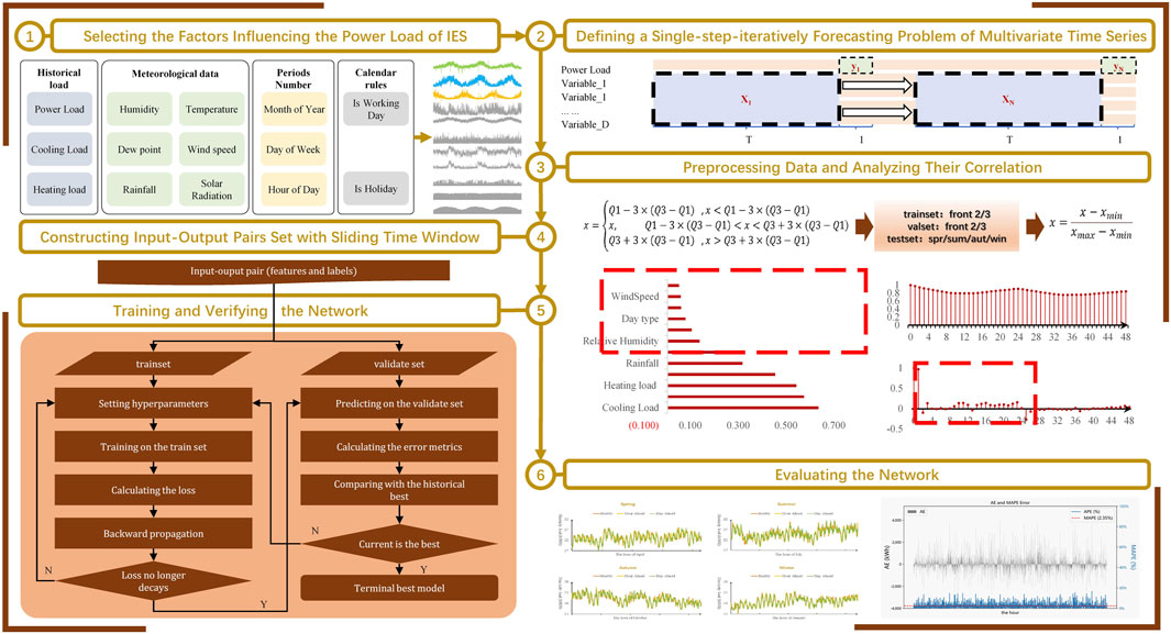
Figure 1. Short-term power forecasting framework for integrated energy system.
2.1 Selecting the factors influencing the power load of IES
The IES can be categorized into three tiers: inter-district, regional, and user-levels based on the scale of the region (Song et al., 2022). However, a uniform division standard regarding the regional size, voltage level, and other relevant characteristics has not been established for both regional-level and user-level IES entities. To address this issue, the framework is applicable to STPLF when dealing with user-level IES such as schools, hospitals, and shopping malls, which particularly prioritize end-use energy consumption. As a result, the research subject within this paper is specifically defined as user-level IES.
In traditional STPLF for power systems, a multitude of factors including seasonal changes, weather patterns, holiday effects, economic growth levels, and consumer electricity consumption behaviors significantly impact the predictions. These factors contribute to unique characteristics such as substantial data volatility, strong nonlinearity, and high uncertainty in STPLF outcomes (Eren and Küçükdemiral, 2024). To refine prediction accuracy, it is essential to comprehensively examine the underlying laws governing load variations in power grids and meticulously analyze these influential elements. In particular, there are complex interactions between meteorological conditions, day types, and short-term load fluctuations (Sheng et al., 2023). By adopting this holistic analytical approach, conventional STPLF methodologies ensure that the influence of all critical variables—meteorology, periodic series, calendar rules, and historical loads—are adequately addressed when forecasting future loads (Zhu et al., 2022).
Typically, meteorological factors encompass elements such as temperature, humidity, solar radiation, among others. The periodic series number denotes the position of a given data point within a longer time horizon that exhibits a periodic pattern. It mainly includes the hour of the day, the day of the week, and the month of the year in ordinal sequence. Calendar rules refer to the specific significance that certain moments carry within the local cultural and political context, examples being weekends or holidays like Christmas. Historical power loads represent the patterns and trends exhibited by observed power load values at various historical timestamps within a time series.
In addition to electrical equipment that has long been prevalent in daily life, such as refrigerators and electric air conditioners, a user-level IES may also incorporate various energy conversion devices like combined heat and power systems. This integration introduces the coupling relationship between power loads, heating loads, and cooling loads, which can be complementary, interdependent, or exhibit more intricate nonlinear relationships. Consequently, given the influence of terminal cooling and heating energy loads on power load, The set of influencing factors for user-level IES is constructed as Figure 2.
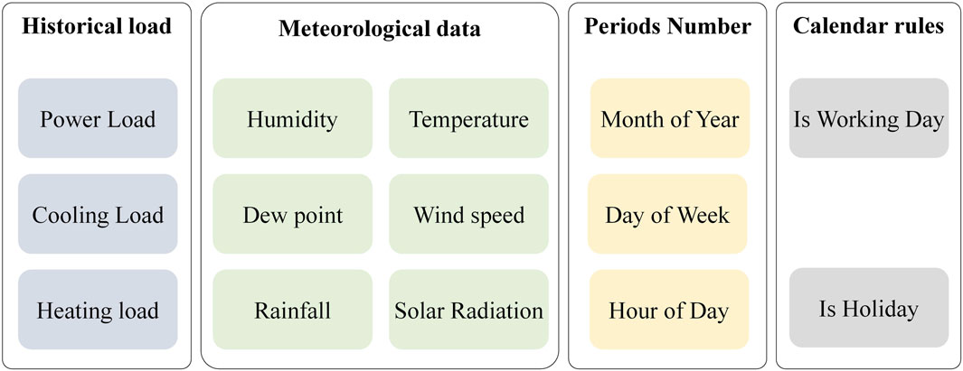
Figure 2. Factors impacting short-term load forecasting in IES.
2.2 Defining a single-step-iteratively forecasting problem of multivariate time series
STPLF typically views power load at any moment as a random variable. Depending on the number of such variables considered, forecasting methods are categorized into univariate and multivariate. Univariate methods, exemplified by ARIMA, focus solely on historical loads. Multivariate methods, discussed in Section 2.1, account for multiple influencing factors.
Multivariate forecasting further categorizes inputs into vector-type and matrix-type based on their structure. Vector-type inputs construct a multivariate vector from series of random variables. SVR is a model that utilizes this method. Matrix-type inputs form matrices from sequences of random variables, representing joint multivariate time series, with models like LSTM and TCN fitting this category.
Forecasts can be divided into single-step and multi-step according to the forecasting horizon. Single-step forecasting predicts one time step at a time, while multi-step forecasts multiple steps simultaneously. However, due to inherent complexities, most researchers adopt iterative single-step predictions to forecast multiple steps.
For instance, when predicting twenty-four future steps, an iterative approach first predicts the first step’s load, then uses it as the actual value to predict the second step, repeating this process in a loop for twenty-four iterations to achieve a rolling twenty-four-step prediction.
2.3 Preprocessing data and analyzing their correlation
Data preprocessing plays a pivotal role in enhancing data quality, encompassing tasks such as outlier treatment and normalization, as exemplified by Eqs 1, 2. This preliminary step is followed by correlation analysis to identify the factors closely related to short-term power load, thereby streamlining input variables and boosting forecasting performance.
The Maximal Information Coefficient (MIC) (Reshef et al., 2011) is employed to quantify the correlation between various factors and power load. The fundamental principle of MIC involves using a scatter plot to depict the discrete relationship between two variables. Initially, the current two-dimensional space is partitioned into a certain number of intervals, denoted by a along the x-axis and b along the y-axis, respectively. Subsequently, the joint probability is computed by observing how often data points fall into each resulting square, as illustrated in core Eqs. (3), (4). What differentiates MIC from traditional correlation coefficients such as Pearson is its ability to discern not only linear relationships but also non-linear associations.
Furthermore, this study calculates autocorrelation coefficients and partial autocorrelation coefficients (Kan and Wang, 2010) for power load to scientifically determine the historical window lengths applicable to each time series within the input matrix.
where mic (x; y) represents the MIC value between the variables x and y. Its value ranges from 0 to 1, with a higher value indicating stronger correlation and a value closer to 0 indicating greater independence between them. a and b represent the number of blocks in the x − axis and y − axis directions, respectively. The parameter
2.4 Constructing input-output pairs set with sliding time window
In the context of single-step iterative forecasting for multivariate time series, the method of constructing input-output pairs data for training was depicted as Figure 3. Within the figure,
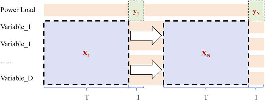
Figure 3. Methodology for constructing input-output pairs using a sliding time Window approach.
2.5 Training and verifying the network
The determination of model parameters occurs through the process of network training and validation, following the selection of a particular forecasting model architecture. The process is meticulously detailed in Figure 4.
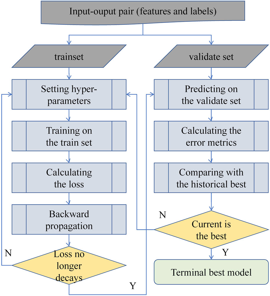
Figure 4. Model training and validation process Flowchart.
The model parameters denote the internal variables that are automatically fine-tuned via backpropagation within the model. In contrast, hyperparameters are predefined settings that govern the training procedure, such as the learning rate for parameter optimization and architectural attributes of the model. Thus, once the model structure is fixed, it is primarily the tuning of hyperparameters that influences the model’s performance. As depicted in Figure 4, this study acquires the optimal model following these steps. Firstly, grid search (Liashchynskyi and Liashchynskyi, 2019) is employed to systematically set hyperparameters across the search space. Next, the model undergoes training until convergence. Subsequently, the trained model predicts on the training data, with corresponding errors computed and recorded. This iterative cycle continues until the entire hyperparameter space has been explored. Ultimately, the model that yields the minimum error on the validation set is selected as the final model.
The Mean Squared Error (MSE) serves as the error metric during both training and validation phases. The model parameter adjustment algorithm utilizes Adaptive Moment Estimation (ADAM), with a specified learning rate γ of 0.001, as shown in Eq. (5).
where y represents the predicted value of power load.
2.6 Evaluating the network
Model prediction and evaluation involve the process of comparing forecasted power load values, produced by a derived functional forecasting model, against the actual observed power load data. This comparison was made among individual models or various combined models incorporating the same module, employing both error index calculations and visual plotting techniques for analysis.
In order to neutralize dimensional effects, MAPE was utilized primarily as the primary error metric. To provide a more comprehensive assessment, MAE and RMSE are also calculated. The specific formulas for these error measures are detailed in Eqs. (6)–(8).
3 RALT hybrid network
In this section, a RALT hybrid architecture is methodically devised through the incorporation of residual connections within the fundamental structures of both LSTM and TCN modules. The integration is purposefully undertaken to enhance their intrinsic abilities to process sequential information. Moreover, an attention mechanism is appended to synergistically blend the complementary strengths of the LSTM and TCN, capitalizing on the parallel processing agility of the TCN alongside the capacity of LSTM to capture long-term dependencies. Thus, the network is equipped with the adaptive capacity to delve into and emphasize the most pertinent segments within time series data in real-time.
3.1 Residual connection
Residual connections have been consistently demonstrated to effectively couple a variable x with its transformed version, which is instrumental in mitigating the gradient vanishing issue prevalent in deeper networks (Shafiq and Gu, 2022). This not only accelerates convergence rates but also enhances the model’s generalization capabilities. The calculation method for residual connections is encapsulated by Eq. (9).
The RALT hybrid network integrated residual connections into LSTM and TCN architectures, thereby allowing them to capture more direct coupling information between input variables and their transformations. This approach facilitates a reduction in the training time of the models and contributes to improved computational efficiency when constructing deeper neural networks.
3.2 Residual LSTM
LSTM enhances the general RNN architecture by incorporating three gates that regulate the flow of information including input gate, forget gate, and output gate. The mechanism of information transfer within an LSTM cell is depicted in the lower right section of Figure 5, accompanied by a corresponding formula presented as Eqs. (10)–(15).
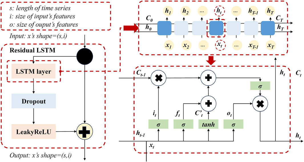
Figure 5. Illustration of a Causal Convolution Process with 2 Hidden Layers, Each Having a Convolution Kernel Size k = 3 and Sequential Dilation Coefficients d = 1, 2, and 3.
In Figure 5, it can be observed that the modified residual structure consists of an LSTM layer, followed by a Dropout layer for random deactivation and topped off with a LeakyReLU activation function.
where [⋅] represents the dot product operation of vectors. [,] represents vector concatenation. i, f, and o represents the input gate, output gate, and forget gate, respectively.
3.3 Residual TCN
TCN, a one-dimensional fully connected convolutional network, is primarily characterized by its use of causal convolutions. It deviates from conventional one-dimensional convolutions in that it applies causal filtering and remains indifferent to the length of input time series (Bai et al., 2018). Figure 6 elucidates this process for a causal convolution with 2 hidden layers, each having a convolution kernel size k of 3 and layer-wise dilation coefficients d incrementing from 1 to 3.
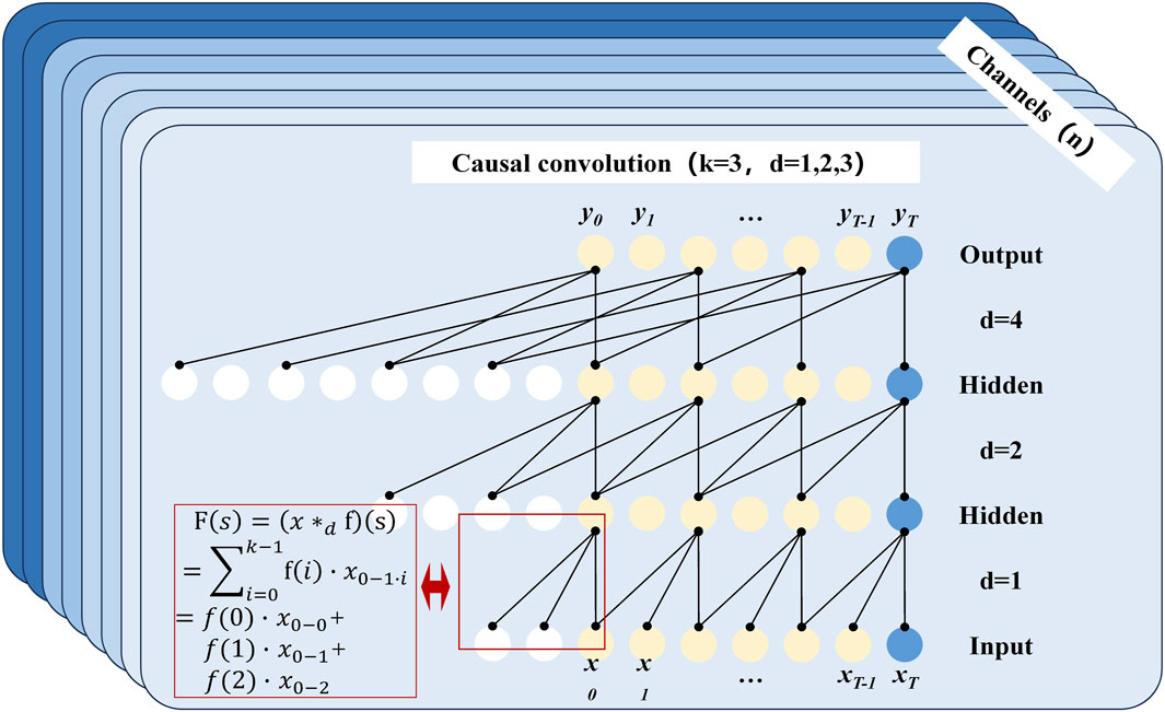
Figure 6. Schematic representation of the residual LSTM architecture.
In Figure 6, channels denote the number of features at each corresponding time step. The red box in the lower left visually depicts the initial convolution operation whose general form is detailed in Eq. (16). The nature of the convolution operation necessitates forward padding of the time series’ head with data to complete the process. Thus, the white circle signifies the number of forward-padded data points, which equals (k − 1)dt. Conversely, the blue circle represents the tail of the time series, which is not padded backward with zeros to ensure that information aggregation flows unidirectionally from past to future. This principle underpins causal convolution and explains why the output sequence retains the same length as the input layer.
where [∗] represents the convolution operation. dt represents the dilation factor. k denotes the size of the convolution kernel. f(t) represents the tth element on the convolution kernel. s and i denote the sth and ith time steps, respectively.
The Residual TCN architecture specifically tailored for this paper is illustrated in Figure 7. It consists of a sequential arrangement of seven identical residual blocks, each with incrementally varying dilation coefficients dt. This design ensures that the network maintains its receptive field while benefiting from the depth and expressiveness of the stacked convolutional layers through residual connections. The incremental dilation across the residual blocks allows the model to capture both short-term and long-term dependencies in the time series data effectively, thereby enhancing the forecasting performance.
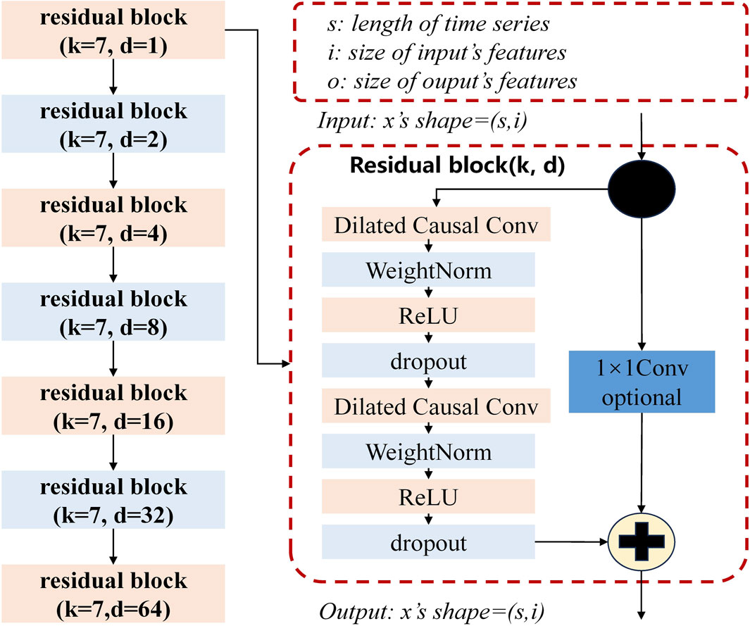
Figure 7. Schematic Illustration of the TCN Architecture with 7 Identically Structured Residual Blocks in Series, Each Having Different Dilation Coefficients d.
3.4 Attention mechanism
The attention mechanism has garnered significant interest and application following the introduction of the transformer model by Vaswani et al. (Vaswani et al., 2017), which is premised on emulating human cognition to selectively concentrate on pertinent areas (Niu et al., 2021). The computational process of this attention mechanism can be articulated as follows. It involves calculating relevance scores between each input element and the focus of attention, converting these scores into probability distributions, and ultimately deriving a weighted sum of the initial inputs based on the score expectations.
The bilinear model (Kim et al., 2018) was employed for computing relevance scores. The formulation of the attention mechanism is shown in Eqs. (17)–(20):
where
3.5 Residual and attentive LSTM-TCN
The combined TCN-LSTM structure, reinforced by residual links and an attention system, is displayed in Figure 8. This design arises from the aim to utilize the benefits of both temporal TCN and LSTM. TCN is particularly skilled at identifying short-range relationships within time series because of their widened causal convolutions. Meanwhile, LSTM is proficient in managing long-range dependencies using their cell states and gate controls.
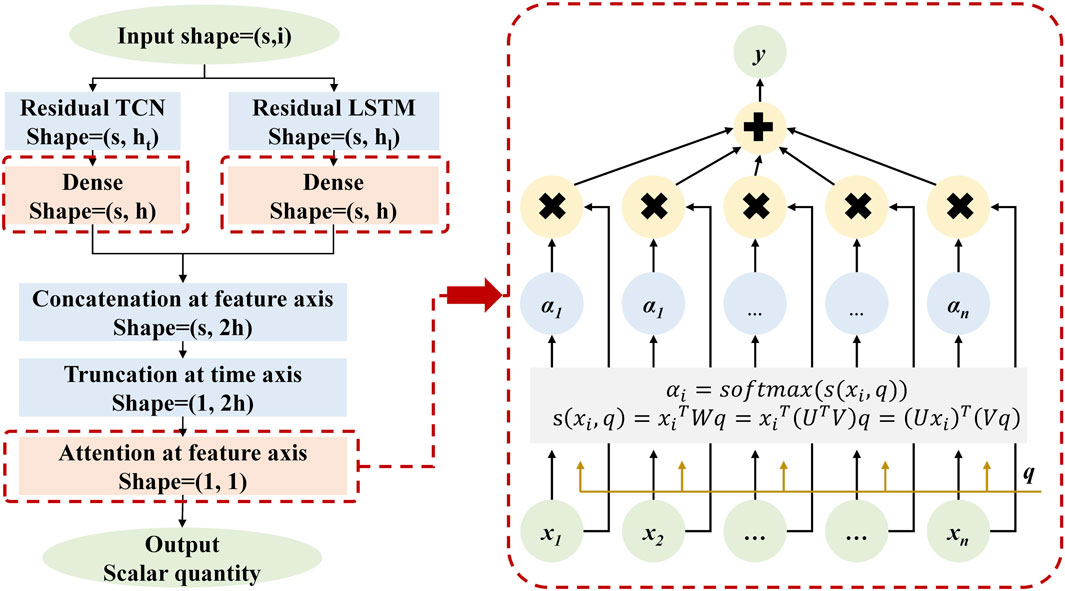
Figure 8. Schematic representation of the RALT hybrid network: Residual and attentive LSTM-TCN.
Initially, the input tensor, characterized by the length of the time series s and the dimensionality of the input attributes i, is concurrently processed by independent Residual TCN and Residual LSTM modules. Here, ht and hl denote the respective numbers of output neurons for each submodule. This two-input approach promotes the model to utilize two time series processing methods, taking advantage of the unique advantages of each method.
Following this, the ensuing outputs from these residual units are concatenated through a fully-connected layer, wherein h represents the cumulative number of output neurons subsequent to concatenation. This fusion stage empowers the network to amalgamate the heterogeneous patterns discerned by the individual layers, fostering a more comprehensive understanding.
Subsequently, a vector concatenation operation is executed along the feature dimension, fusing the learned representations from the disparate models. This is followed by temporal tail pruning, which retains solely the feature vector associated with the terminal time step. This procedure ensures that the condensed representation encapsulates the essence of the entire sequence while preserving a tractable scale.
Finally, a cross-feature attention mechanism is used to dynamically evaluate and weight the importance of different features. This merging approach adaptively maintains healthy competition between TCN and LSTM internally, allowing them to work better together to improve predictive performance.
4 Case study
4.1 Environment of the experiment
The experimental platform was equipped with a Windows operating system, an AMD Ryzen 5 4600H processor running at a clock speed of 3.00 GHz, an NVIDIA GeForce GTX 1650Ti graphics card with 4 GB of dedicated video memory, and 16 GB of Random Access Memory (RAM). The experiments was systematically executed in a sequential order, adhering to the progression of the IES-STPLF methodology, which is supported by the Python programming language and leverages the Pytorch library.
4.2 Data source
The open-source dataset from the 2017 to 2019 period, comprising user-level IES data sourced from Arizona State University’s Tempe Campus in the United States which obtained from (dat, 2022), was chosen as a case study due to its distinct characteristics and relevance to this research. The campus is situated in the southwestern U.S., an area characterized by a hot climate where electric air conditioning units are extensively employed to meet substantial cooling energy demands. Notably, these electric air conditioners also provide heating functionality, thereby optimizing equipment utilization. This unique combination results in a typical user-level IES scenario with a strong interdependence among electricity, cooling, and heating loads.
In this specific case, the dataset from the first 2 years (2017–2018) was partitioned into validation and training sets at a ratio of 7:3, respectively. Meanwhile, the data collected during the last year (2019) served as the test set for experimental evaluation.
4.3 Setups of comparison experiment and selection of model parameters
In this paper, two sets of experiments were set up to compare the differences between the proposed model and other models. One set of baseline experiments was used to compare the differences between the proposed model and other traditional models, and the other set of ablation experiments was used to compare the differences between the proposed model and single submodels within it.
In the series of baseline comparison experiments, four conventional models were selected to serve as benchmarks: ARIMAX, SVR, MLP, and GRU. To guarantee a fair and rigorous evaluation, the principal parameters of these benchmark models underwent meticulous optimization through a grid search method, and the comprehensive results of this process have been documented in Table 1. For ARIMAX model, the autoregressive order p, moving average order q, and degree of differencing da was guided by the minimization of the Akaike Information Criterion, thereby embodying a systematic and statistically informed model identification procedure. With respect to SVR, the adoption of the radial basis function kernel was motivated by its efficacy in addressing non-linear relationships. The regularization parameter λ was set at 1,000, aimed at achieving an optimal balance between model complexity and generalizability, whereas the tolerance bandwidth σ was precisely adjusted to 0.1 to effectively capture the subtle patterns inherent in the data. MLP structure was composed of two hidden layers, each containing 64 and 32 neurons, specifically designed to facilitate intricate feature extraction and transformation. GRU incorporated a single hidden layer that was strengthened by the Rectified Linear Unit (ReLU) activation function, introducing non-linearity and mitigating the issue of vanishing gradients. Moreover, a dropout rate ρ of 0.2 was strategically applied to bolster regularization and deter overfitting during the training phase.
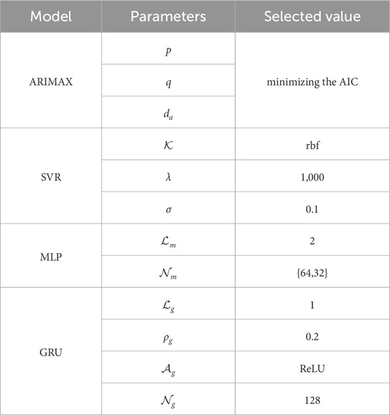
Table 1. Baseline model parameter Configurations.
In the ablation experiment, two key submodules of the proposed RALT model, residual LSTM and residual TCN, were optimized in detail. In Table 2, the search range of each parameter is shown in detail and the final selected optimal value.
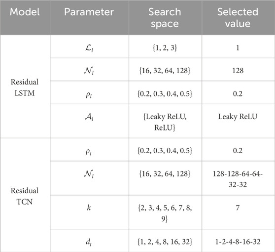
Table 2. Chosen submodule parameters for the proposed model.
For residual LSTM, the number of hidden layers
For the residual TCN, the dropout rate ρl was selected as 0.2 from {0.2, 0.3, 0.4, 0.5} to ensure the robustness of model training. Secondly, according to the residual TCN neuron structure presents unique hierarchical characteristics, the number of neurons
5 Result and discussion
5.1 Analysis of correlation
(Reshef et al., 2011) proposed that the function structure of MIC is similar to the square of the determination coefficient, so the similarity score obtained is also similar. In view of the fact that feature screening is not an outstanding contribution of this paper, reasonable simplification is carried out when feature screening is realized according to the MIC value results (Cui and Wang, 2022). The empirical interval of correlation strength recognized by statisticians was referred to, which includes weak correlation interval (0-0.2), medium correlation interval (0.2–0.8) and strong correlation interval (0.8–1) (Kutner et al., 2005). Therefore, features that are weakly correlated with power load
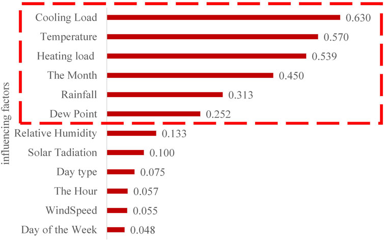
Figure 9. Maximum mutual information coefficient analysis between influencing factors and power load.
As shown in Figure 10, through in-depth analysis of the time series, significant daily cycle characteristics of the power load were revealed. Specifically, there is a strong correlation effect between the power load at the current time of observation (in hours) and its historical load at the same time in the past. Despite the inherent daily periodicity of power loads, considering a broader time window can serve to mitigate random fluctuations effectively, particularly when short-term data encounters outliers or experiences significant noise interference. Given these results, the length value
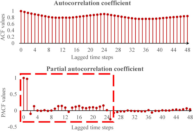
Figure 10. Power load autocorrelation and partial autocorrelation coefficients analysis.
In order to discuss the influence of feature input on the prediction performance, the length value
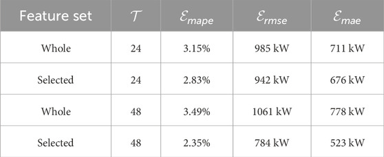
Table 3. Comparison of filtered and unfiltered features.
5.2 Analysis of prediction performance
In order to evaluate the performance of the model rigorously, as shown in Figure 11, a period-by-period comparative analysis between the predicted load curve and the actual load curve is performed. Owing to constraints in visual density when depicting full-year data within line charts, generating such representations frequently leads to excessively cluttered visuals that hinder efficient comparisons of subtle differences between forecasted and actual load patterns, thereby compromising their inherent intuitive value for data visualization purposes. To circumvent this issue, a strategy is adopted to analyze detailed curve comparisons by extracting a subset of representative data from a single month within each season. It can be analyzed from the figure that the impact of the difference in the variation trend of power load on the forecast results is multifaceted, as follows:
• The overall load levels during spring and summer exhibit a significantly higher amplitude compared to those in autumn and winter, thus leading to considerable deviations from the actual values at peak periods.
• Spring and autumn display analogous and moderate load variation trends, consequently yielding a relatively better fit in the forecast results.
• By contrast, summer and winter demonstrate notably distinct load variation trends with relatively sharper fluctuations, resulting in increased numbers of deviation points in the forecasts during periods of change.
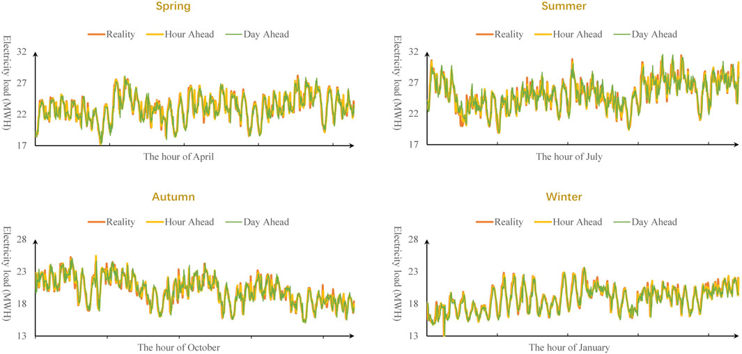
Figure 11. Model-Based Prediction vs. Actual Curve Comparison.
To clarify, these observations do not imply any inherent issues with the prediction results. Instead, they precisely elucidate the reasons behind the challenge of accurately predicting short-term power loads and hint at how exploring the model’s contributions could potentially enhance the precision of short-term load predictions.
Then, as shown in Figure 12, a histogram of the absolute error and absolute percentage error for each time step is plotted. The prediction performance of the model is analyzed directly from the perspective of error. The results show that:
• Absolute errors are larger in some periods of the day than in other periods. Combined with Figure 11 and actual data analysis, these larger errors are precisely located at the sharp fluctuations of load.
• The MAPE error remains low, demonstrating that the model is able to show the stability of accurate predictions across the entire test set.
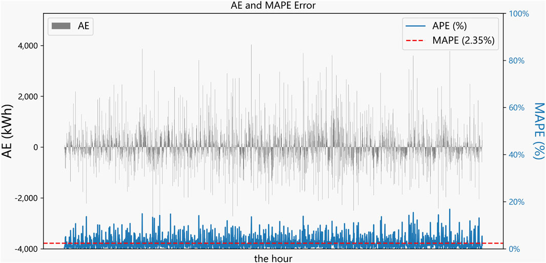
Figure 12. Absolute and percentage absolute errors of IES-STPLF framework.
Finally, as shown in Table 4, three prediction error indicators (MAPE, MAE, RMSE) are calculated for each season. Quantitative analysis of the results shows that:
• The error in spring and autumn is generally smaller than that in summer and winter, revealing the load characteristics of IES with “high in summer, low in winter and flat in spring as well as autumn”
• High volatility is an important factor leading to the increase of prediction error, and handling the volatility well is the key to improving the prediction accuracy.
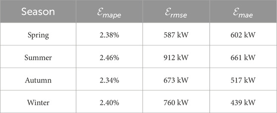
Table 4. Seasonal error metrics for STPLF using the proposed model.
5.3 Analysis of superiority
Baseline comparison results verify the superiority of the model over other traditional models, as shown in Table 5 and Figure 13. The qualitative analysis from Figure 13 shows that the model in this paper has the best fitting effect. Table 5 can be used to quantitatively analyze the difference in forecasting effect between the proposed model and other models. The results show that:
• ARIMAX and SVR show relatively high MAPE values (4.05% and 4.00%) over the entire test set, confirming their limitations in handling complex and large sample datasets.
• GRU and MLP show relatively moderate MAPE values (2.79% and 2.87%) over the entire test set, which validates their strong fitting ability in dealing with nonlinear relationships.
• Across the entire test set, the model achieves the lowest MAPE value at 2.35%, which primarily demonstrates its ability to consistently outperform other models across all indicators during both summer and winter months. This outcome effectively validates the model’s superiority in managing volatility.
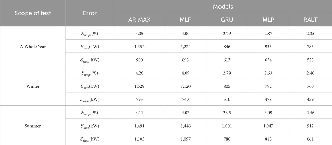
Table 5. Error metrics in baseline experiment.
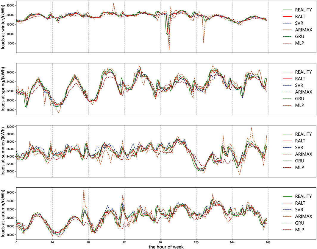
Figure 13. Line graph comparison: Load curve performance in the baseline experiment.
5.4 Analysis of combination mechanism
To verify the effect of attention mechanisms on the combination of LSTM and TCN, a set of ablation experiments are performed whose parameters were set in Section 4.3. The results are shown in Figure 14 and Table 6.
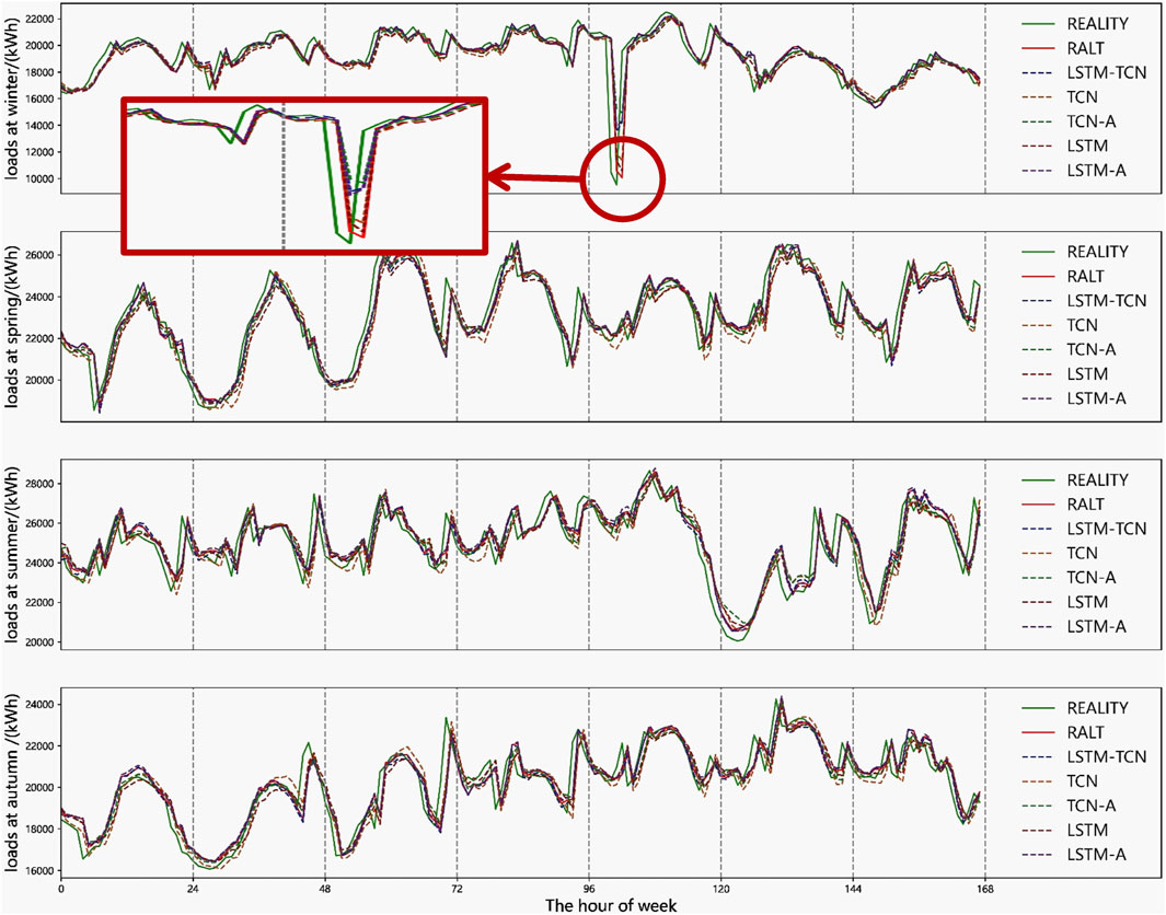
Figure 14. Line graph comparison: Load curve performance in the ablation experiment.
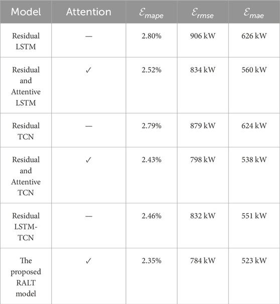
Table 6. Error metrics in ablation experiment.
Figure 14 randomly samples seven consecutive days of load forecast data from four seasons, and plots the comparison curve between predicted load and actual load. Qualitative analysis shows that:
• TCN is better than LSTM in general trend fitting, but it is difficult to deal with fluctuations on a small time scale. This is limited by the receptive field of TCN, and although the convolution kernel size can be adjusted to improve it, it is difficult to find a better choice in the same training time.
• Compared with TCN, LSTM is better at the fitting of fine details, and the extraction capability of long-term dependence enables it to better process local information.
• The RALT model demonstrates superior adaptability to fluctuations compared to others, particularly excelling in capturing sharp load variations as exemplified within the red box in Figure 14. This enhanced capability to embrace volatility directly translates into more accurate forecasting outcomes.
Two control groups are listed to explore the influence of combination mechanism on prediction results, as shown in Table 6. Among them, one group is whether the combination is produced, and the other is whether the attention mechanism is used. In the table, − indicates that the attention mechanism is not used, and √ indicates that the attention mechanism is used. The results in the table can be quantitatively analyzed:
• The use of hybrid structures can indeed improve the accuracy of prediction models. When the mixed structure is not used, the MAPE of Residual LSTM is 2.80% and the MAPE of Residual TCN is 2.79%. When combined directly in parallel, the Residual LSTM-TCN’s MAPE is 2.46%, a decrease of about 0.34 percentage points.
• The introduction of attention mechanisms can indeed improve the accuracy of predictive models. The MAPE of Residual and Attentive LSTM is 2.52%, which is 0.28 percentage points lower than when no attention mechanism is used, and the MAPE of Residual and Attentive TCN is 2.43%, 0.36 percentage points lower in comparison to the case without the attention mechanism. RALT achieved a MAPE of 2.35%, marking a decrease of 0.11 percentage points.
• The MAPE of RALT is 2.35%, which is lower than the single model using attention mechanisms but without mixing (2.52% and 2.43%), and lower than the ordinary parallel combination (2.46%).
These results fully verify the rationality of the combination mechanism. The parallel combination structure through the attention mechanism allows LSTM and TCN to remain competitive while exploiting the advantages of both—LSTM’s long-term dependence on extraction capabilities and TCN’s efficient parallel computing capabilities. Further, higher precision prediction performance is achieved.
6 Conclusion and prospect
In this paper, aiming at the high uncertainty caused by multi-energy coupling of IES, a STPLF problem was studied. This problem is described as univariate iterative prediction of multivariate time series, and an RALT hybrid neural network was proposed to solve this problem. With the RALT network as the core, a STPLF framework was proposed to realize the whole process encapsulation of original input, data processing, model training and prediction output. The proposed framework not only considers the correlation between heating and cooling load as well as power load to be suitable for multi-energy coupled IES, but also cleverly combines the advantages of LSTM and TCN to adapt to short-term power load volatility through attention mechanism. The RALT network combines residual LSTM and residual TCN in parallel by means of attention mechanism, which not only ensures their effective competition in the same prediction problem, but also incorporates their prediction differences caused by different mechanisms. This combination empowers the RALT network to harness both the high-performance parallel processing capabilities of TCN and the superior long-term dependency recognition attributes of LSTM, thereby augmenting its overall predictive proficiency. The results of a real case study of a user-level IES show that the MAPE of the proposed framework on the test set is 2.35%. This loss is lower than the average level of the traditional methods (3.43%) and the average level of the uncombined single submodules (2.80%), which verifies the superiority. Meanwhile, the results of the case study also show that the proposed framework has a better fitting effect in the short-term power load fluctuation, which verifies the robustness.
In the future, comprehensive places that integrate living, working and production regionally can effectively smooth out the peak-valley difference of power grid load and improve equipment utilization. IES of typical scenes such as hospitals, campuses, industrial parks and commercial venues are gradually built as preliminary pilots. In order to supply a variety of energy sources, the coordination and interaction between the subsystems are becoming closer and closer. The method proposed in this paper can be effectively applied to this to enhance the load prediction results. Although all the core work has been described in detail, in fact, there are still some directions that are considered to improve the method in the future. The proposed framework can be improved by: 1) Considering the signal decomposition-reconstruction method which can mini more prior knowledge of load characteristics to improve forecasting performance; 2) Considering multi-task learning method which can predicting multiple loads concurrently to fit richer scenarios; 3) Considering the new energy generation forecasting which can achieve the joint forecast of the source-load to provide more reference information for the balance of supply and demand.
Data availability statement
Publicly available datasets were analyzed in this study. This data can be found here: https://cm.asu.edu/.
Author contributions
HL: Methodology, Writing–original draft, Writing–review and editing. SL: Methodology, Project administration, Validation, Writing–review and editing. YW: Validation, Writing–review and editing. YX: Validation, Writing–review and editing. ZP: Validation, Writing–review and editing. ML: Conceptualization, Project administration, Supervision, Writing–review and editing.
Funding
The author(s) declare that no financial support was received for the research, authorship, and/or publication of this article.
Conflict of interest
The authors declare that the research was conducted in the absence of any commercial or financial relationships that could be construed as a potential conflict of interest.
Publisher’s note
All claims expressed in this article are solely those of the authors and do not necessarily represent those of their affiliated organizations, or those of the publisher, the editors and the reviewers. Any product that may be evaluated in this article, or claim that may be made by its manufacturer, is not guaranteed or endorsed by the publisher.
References
Abiodun, O. I., Jantan, A., Omolara, A. E., Dada, K. V., Mohamed, N. A., and Arshad, H. (2018). State-of-the-art in artificial neural network applications: a survey. Heliyon 4, e00938. doi:10.1016/j.heliyon.2018.e00938
Agga, A., Abbou, A., Labbadi, M., El Houm, Y., and Ali, I. H. O. (2022). Cnn-lstm: an efficient hybrid deep learning architecture for predicting short-term photovoltaic power production. Electr. Power Syst. Res. 208, 107908. doi:10.1016/j.epsr.2022.107908
Akhtar, S., Shahzad, S., Zaheer, A., Ullah, H. S., Kilic, H., Gono, R., et al. (2023). Short-term load forecasting models: a review of challenges, progress, and the road ahead. Energies 16, 4060. doi:10.3390/en16104060
Alzubaidi, L., Zhang, J., Humaidi, A. J., Al-Dujaili, A., Duan, Y., Al-Shamma, O., et al. (2021). Review of deep learning: concepts, cnn architectures, challenges, applications, future directions. J. big Data 8, 53–74. doi:10.1186/s40537-021-00444-8
Bai, S., Kolter, J. Z., and Koltun, V. (2018). An empirical evaluation of generic convolutional and recurrent networks for sequence modeling. CoRR abs/1803.01271.
Bianchi, F. M., Maiorino, E., Kampffmeyer, M. C., Rizzi, A., and Jenssen, R. (2017). An overview and comparative analysis of recurrent neural networks for short term load forecasting. CoRR abs/1705.04378.
Box, G. (2013). “Box and jenkins: time series analysis, forecasting and control,” in A very British affair: six britons and the development of time series analysis during the 20th century (Springer), 161–215.
Box, G. E., and Pierce, D. A. (1970). Distribution of residual autocorrelations in autoregressive-integrated moving average time series models. J. Am. Stat. Assoc. 65, 1509–1526. doi:10.1080/01621459.1970.10481180
Cai, C., Li, Y., Su, Z., Zhu, T., and He, Y. (2022). Short-term electrical load forecasting based on vmd and gru-tcn hybrid network. Appl. Sci. 12, 6647. doi:10.3390/app12136647
Cai, M., Pipattanasomporn, M., and Rahman, S. (2019). Day-ahead building-level load forecasts using deep learning vs. traditional time-series techniques. Appl. energy 236, 1078–1088. doi:10.1016/j.apenergy.2018.12.042
Campus metabolism (2022). Campus metabolism. Available at: https://cm.asu.edu.
Chen, B., and Wang, Y. (2021). Short-term electric load forecasting of integrated energy system considering nonlinear synergy between different loads. IEEE Access 9, 43562–43573. doi:10.1109/access.2021.3066915
Chen, L., Xu, Q., Yang, Y., Gao, H., and Xiong, W. (2022). Community integrated energy system trading: a comprehensive review. J. Mod. Power Syst. Clean Energy 10, 1445–1458. doi:10.35833/mpce.2022.000044
Cheng, H., Hu, X., Wang, L., Liu, Y., and Yu, Q. (2019). Review on research of regional integrated energy system planning. Automation Electr. Power Syst. 43, 2–13. doi:10.7500/AEPS20180416006
Cho, K., van Merrienboer, B., Gülçehre, Ç., Bougares, F., Schwenk, H., and Bengio, Y. (2014). Learning phrase representations using RNN encoder-decoder for statistical machine translation. CoRR abs/1406.1078.
Cui, S., and Wang, X. (2022). Multivariate load forecasting in integrated energy system based on maximal information coefficient and multi-objective stacking ensemble learning. Electr. Power Autom. Equipment/Dianli Zidonghua Shebei 42, 32–39+81. doi:10.16081/j.epae.202202025
Ding, T., Jia, W., Shahidehpour, M., Han, O., Sun, Y., and Zhang, Z. (2022). Review of optimization methods for energy hub planning, operation, trading, and control. IEEE Trans. Sustain. Energy 13, 1802–1818. doi:10.1109/tste.2022.3172004
Eren, Y., and Küçükdemiral, İ. (2024). A comprehensive review on deep learning approaches for short-term load forecasting. Renew. Sustain. Energy Rev. 189, 114031. doi:10.1016/j.rser.2023.114031
Fan, H., Wang, C., Liu, L., and Li, X. (2022). Review of uncertainty modeling for optimal operation of integrated energy system. Front. energy Res. 9, 641337. doi:10.3389/fenrg.2021.641337
Guo, J., Wu, D., Wang, Y., Wang, L., and Guo, H. (2023). Co-optimization method research and comprehensive benefits analysis of regional integrated energy system. Appl. Energy 340, 121034. doi:10.1016/j.apenergy.2023.121034
Han, X., Su, J., Hong, Y., Gong, P., and Zhu, D. (2022). Mid-to long-term electric load forecasting based on the emd–isomap–adaboost model. Sustainability 14, 7608. doi:10.3390/su14137608
Hornik, K., Stinchcombe, M., and White, H. (1989). Multilayer feedforward networks are universal approximators. Neural Netw. 2, 359–366. doi:10.1016/0893-6080(89)90020-8
Javed, U., Ijaz, K., Jawad, M., Khosa, I., Ansari, E. A., Zaidi, K. S., et al. (2022). A novel short receptive field based dilated causal convolutional network integrated with bidirectional lstm for short-term load forecasting. Expert Syst. Appl. 205, 117689. doi:10.1016/j.eswa.2022.117689
Kan, R., and Wang, X. (2010). On the distribution of the sample autocorrelation coefficients. J. Econ. 154, 101–121. doi:10.1016/j.jeconom.2009.06.010
Kang, L., Wu, X., Yuan, X., and Wang, Y. (2022). Performance indices review of the current integrated energy system: from history and projects in China. Sustain. Energy Technol. Assessments 53, 102785. doi:10.1016/j.seta.2022.102785
Ke, Y., Liu, J., Meng, J., Fang, S., and Zhuang, S. (2022). Comprehensive evaluation for plan selection of urban integrated energy systems: a novel multi-criteria decision-making framework. Sustain. Cities Soc. 81, 103837. doi:10.1016/j.scs.2022.103837
Ke, Y., Tang, H., Liu, M., Meng, Q., and Xiao, Y. (2023). Optimal sizing for wind-photovoltaic-hydrogen storage integrated energy system under intuitionistic fuzzy environment. Int. J. Hydrogen Energy 48, 34193–34209. doi:10.1016/j.ijhydene.2023.05.2452023.05.245
Li, J., Li, D., Zheng, Y., Yao, Y., and Tang, Y. (2022). Unified modeling of regionally integrated energy system and application to optimization. Int. J. Electr. Power & Energy Syst. 134, 107377. doi:10.1016/j.ijepes.2021.107377
Li, K., Huang, W., Hu, G., and Li, J. (2023). Ultra-short term power load forecasting based on ceemdan-se and lstm neural network. Energy Build. 279, 112666. doi:10.1016/j.enbuild.2022.112666
Li, L., Ota, K., and Dong, M. (2017). “Everything is image: cnn-based short-term electrical load forecasting for smart grid,” in 2017 14th international symposium on pervasive systems, algorithms and networks & 2017 11th international conference on frontier of computer science and technology & 2017 third international symposium of creative computing (ISPAN-FCST-ISCC) (IEEE), 344–351.
Liashchynskyi, P., and Liashchynskyi, P. (2019). Grid search, random search, genetic algorithm: a big comparison for NAS. CoRR abs/1912.06059.
Lin, J., Ma, J., Zhu, J., and Cui, Y. (2022). Short-term load forecasting based on lstm networks considering attention mechanism. Int. J. Electr. Power & Energy Syst. 137, 107818. doi:10.1016/j.ijepes.2021.107818
Liu, M., Qin, H., Cao, R., and Deng, S. (2022a). Short-term load forecasting based on improved tcn and densenet. IEEE Access 10, 115945–115957. doi:10.1109/access.2022.3218374
Liu, X., Yue, Y., Huang, X., Xu, W., and Lu, X. (2022b). A review of wind energy output simulation for new power system planning. Front. Energy Res. 10, 942450. doi:10.3389/fenrg.2022.942450
Lv, J., Zhang, S., Cheng, H., Han, F., Yuan, K., Song, Y., et al. (2021). Review on district-level integrated energy system planning considering interconnection and interaction. Proc. CSEE 41, 4001–4021.
Ma, X., Peng, B., Ma, X., Tian, C., and Yan, Y. (2023). Multi-timescale optimization scheduling of regional integrated energy system based on source-load joint forecasting. Energy 283, 129186. doi:10.1016/j.energy.2023.129186
Kutner, M. H., Nachtsheim, C. J., Neter, J., and Li, W. (2005). Applied linear statistical models. McGraw-hill.
Niu, D., Yu, M., Sun, L., Gao, T., and Wang, K. (2022). Short-term multi-energy load forecasting for integrated energy systems based on cnn-bigru optimized by attention mechanism. Appl. Energy 313, 118801. doi:10.1016/j.apenergy.2022.118801
Niu, Z., Zhong, G., and Yu, H. (2021). A review on the attention mechanism of deep learning. Neurocomputing 452, 48–62. doi:10.1016/j.neucom.2021.03.091
Noble, W. S. (2006). What is a support vector machine? Nat. Biotechnol. 24, 1565–1567. doi:10.1038/nbt1206-1565
Qiao, Y., Hu, F., Xiong, W., Guo, Z., Zhou, X., and Li, Y. (2023). Multi-objective optimization of integrated energy system considering installation configuration. Energy 263, 125785. doi:10.1016/j.energy.2022.125785
Reshef, D. N., Reshef, Y. A., Finucane, H. K., Grossman, S. R., McVean, G., Turnbaugh, P. J., et al. (2011). Detecting novel associations in large data sets. science 334, 1518–1524. doi:10.1126/science.1205438
Şeker, M. (2022). Long term electricity load forecasting based on regional load model using optimization techniques: a case study. Energy Sources, Part A Recovery, Util. Environ. Eff. 44, 21–43. doi:10.1080/15567036.2021.1945170
Shafiq, M., and Gu, Z. (2022). Deep residual learning for image recognition: a survey. Appl. Sci. 12, 8972. doi:10.3390/app12188972
Sheng, Z., An, Z., Wang, H., Chen, G., and Tian, K. (2023). Residual lstm based short-term load forecasting. Appl. Soft Comput. 144, 110461. doi:10.1016/j.asoc.2023.110461
Sherstinsky, A. (2020). Fundamentals of recurrent neural network (rnn) and long short-term memory (lstm) network. Phys. D. Nonlinear Phenom. 404, 132306. doi:10.1016/j.physd.2019.132306
Song, D., Meng, W., Dong, M., Yang, J., Wang, J., Chen, X., et al. (2022). A critical survey of integrated energy system: summaries, methodologies and analysis. Energy Convers. Manag. 266, 115863. doi:10.1016/j.enconman.2022.115863
Tarmanini, C., Sarma, N., Gezegin, C., and Ozgonenel, O. (2023). Short term load forecasting based on arima and ann approaches. Energy Rep. 9, 550–557. doi:10.1016/j.egyr.2023.01.060
Vaswani, A., Shazeer, N., Parmar, N., Uszkoreit, J., Jones, L., Gomez, A. N., et al. (2017). “Attention is all you need,” in Advances in neural information processing systems. Editors I. Guyon, U. V. Luxburg, S. Bengio, H. Wallach, R. Fergus, S. Vishwanathanet al. (Curran Associates, Inc.), 30.
Wang, W., Wang, D., Jia, H., Chen, Z., Guo, B., Zhou, H., et al. (2016). Review of steady-state analysis of typical regional integrated energy system under the background of energy internet. Proc. CSEE 36, 3292–3305.
Yang, T., Zhao, L., and Wang, C. (2019). Review on application of artificial intelligence in power system and integrated energy system. Automation Electr. Power Syst. 43, 2–14.
Yu, Y., Si, X., Hu, C., and Zhang, J. (2019). A review of recurrent neural networks: lstm cells and network architectures. Neural Comput. 31, 1235–1270. doi:10.1162/neco_a_01199
Zhang, W., Gu, L., Shi, Y., Luo, X., and Zhou, H. (2022). A hybrid svr with the firefly algorithm enhanced by a logarithmic spiral for electric load forecasting. Front. Energy Res. 10, 977854. doi:10.3389/fenrg.2022.977854
Zhu, J., Dong, H., Zheng, W., Li, S., Huang, Y., and Xi, L. (2022). Review and prospect of data-driven techniques for load forecasting in integrated energy systems. Appl. Energy 321, 119269. doi:10.1016/j.apenergy.2022.119269
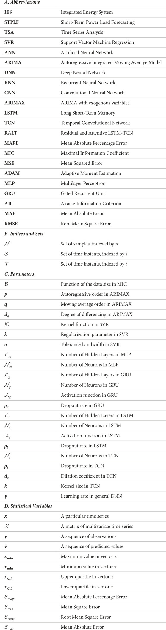
Nomenclature
Keywords: short-term power load forecasting, integrate energy system, long short-term memory, temporal convolutional network, attention mechanism
Citation: Li H, Li S, Wu Y, Xiao Y, Pan Z and Liu M (2024) Short-term power load forecasting for integrated energy system based on a residual and attentive LSTM-TCN hybrid network. Front. Energy Res. 12:1384142. doi: 10.3389/fenrg.2024.1384142
Received: 08 February 2024; Accepted: 15 April 2024;
Published: 10 May 2024.
Edited by:
Haonan Zhang, North China Electric Power University, ChinaReviewed by:
Jianli Zhou, Xinjiang University, ChinaHao Lu, North China Electric Power University, China
Copyright © 2024 Li, Li, Wu, Xiao, Pan and Liu. This is an open-access article distributed under the terms of the Creative Commons Attribution License (CC BY). The use, distribution or reproduction in other forums is permitted, provided the original author(s) and the copyright owner(s) are credited and that the original publication in this journal is cited, in accordance with accepted academic practice. No use, distribution or reproduction is permitted which does not comply with these terms.
*Correspondence: Min Liu, bGl1bWluQGpudS5lZHUuY24=