Abnormal line loss identification and category classification of distribution networks based on semi-supervised learning and hierarchical classification

Line loss refers to the electrical energy that is dissipated as heat during the transmission and distribution of electricity through power lines. However, unusual causes, such as grid topology mismatch and communication failure, can cause abnormal line loss. Efficient abnormal line loss detection contributes not only to minimizing energy wastage and reducing carbon emissions but also to maintaining the stability and reliability of the entire distribution network. In actual situations, the cause of abnormal line loss is not labeled due to the expensive labor cost. This paper proposes a hierarchical abnormal line loss identification and category classification model, considering the unlabeled and unbalanced sample problem. First, an abnormal line loss identification model-based random forest is established to detect whether the line loss is abnormal. Then, an abnormal line loss category classification model is developed with semi-supervised learning for line loss abnormal category classification, considering the unlabeled samples. The real dataset in China is utilized to validate the performance of the proposed model. Its reliability implies the potential to be applied to real-world scenarios to improve the management level and safety of the power grid.

1 Introduction

The line loss rate is an essential indicator of economy and technology in the low-voltage distribution network (DN) (Sayed and Takeshita, 2011; Luo et al., 2021; Sun et al., 2022). With access to distributed generation and flexible load, DN becomes increasingly complex. Meanwhile, with the increasing electricity demand, a certain quantity of line loss in DN is generated. However, limited by the metering accuracy of data acquisition devices and the reliability of transmission systems, line loss identification in DN is usually completed by labor (Jing et al., 2019). Due to the incomplete installation of metering instruments of low-voltage substations and customers (Zhu and Lin, 2021; Raghuvamsi et al., 2022), it is challenging to analyze the causes of line loss.

With the establishment of big data centers and the development of machine learning, power supply corporations have gradually started to analyze line loss based on data-driven models to improve the economic benefits. According to the data source, the data-driven line loss analysis can be divided into user-oriented data analysis and DN substation area data analysis. Gunturi and Sarkar (2021) proposed an electricity theft detection model based on an ensemble machine learning model. The model applied the statistical method of oversampling to solve the over-fitting problem during the training process. Based on the terminal acquisition data, the model could identify the line loss anomaly in a small-scale DN. Buzau et al. (2020) used a user-side line loss identification algorithm based on a hybrid depth neural network to detect non-technical losses. The algorithm integrated a long short-term memory network and a multi-layer sensing machine, which were used for processing the original data and integrating non-time series data. Chen J. D. et al. (2023) established an electricity theft detection model based on a one-dimensional convolutional neural network. It analyzed the non-technical line loss on the user side according to the complete terminal data. The above three methods (Buzau et al., 2020; Gunturi and Sarkar, 2021; Chen J. D. et al., 2023) show a significant role in line loss identification on the user side. However, they are sensitive to the quality of user-side power consumption data and lack of universality.

Regarding line loss identification in DN, a feeder loss estimation method based on the boost k-means model was developed (Chen J. et al., 2023). The analysis index system for line loss was established, and the multi-information index was calculated according to the time series data. The established characteristic indexes were imported into the boost k-means algorithm for clustering calculation, and the outliers were marked as line loss data. Wu et al. (2019) introduced an algorithm of non-technical line loss of DN identification with large samples. Based on the robust neural network model, the proposed method employed an automatic denoising encoder to pre-process data. The RNN model classified the operation data and identified the non-technical line loss value. Yao et al. (2019) analyzed the topology of a low-voltage DN and used the GBDT model to predict the abnormal line loss nodes in the substation area. Based on parameter clustering and deep learning algorithms, the parameter correlation and time series characteristics of a DN were fully considered by Liu et al. (2022) and Zhang et al. (2022). The multi-variate characteristic parameters were utilized to predict line loss events in a DN. When the topology of the DN is clear and the operation parameters are complete, identifying and predicting line loss based on the data-driven algorithm in the substation area can achieve remarkable results.

In actual operation conditions, it is difficult to accurately measure the operational parameters in the distribution network and the accuracy power consumption data (Lin and Abur, 2018; Jiang and Tang, 2020). Zhou et al. (2022) proposed a non-technical line loss identification model based on an AP reconstruction neural network. The model reconstructed and corrected the anomaly data by the AP neural network based on the simulation dataset, followed by a deep neural network to classify the data. Huang et al., (2023) constructed the electrical characteristic index system of theoretical line loss, and the power torque was proposed to identify line loss in the case of missing line data in a DN. However, this method is a supervised learning algorithm, which requires a certain amount of labeled data to train the model. In recent years, analyzing the causes of line loss has become a research focus. Power supply corporations have become interested in the causes of different line loss types. Liang et al. (2022) proposed a line loss interval calculation method based on power flow calculation and linear optimization, which was suitable for datasets with anomalies. This method fully considered the power flow and dispatching information and analyzed the cause of area line loss. Some studies (Wang et al., 2019; Sun et al., 2023) mentioned data-driven algorithms for line loss cause analysis, locating anomalous nodes in the network topology and analyzing the abnormal causes according to parameter deviations.

With the increasing complexity of DNs, the accuracy of traditional line loss identification methods on the overall level of the DN is crucial to guarantee. All data-driven algorithms and statistical methods greatly rely on the data quality and data quantity, especially the labeled data. The unsupervised learning methods, such as the clustering algorithms, do not need the labeled data to detect the abnormal line loss. However, its performance is limited and cannot identify the abnormal category. When the abnormal line loss data occupied the main part of the whole data, the clustering algorithm would directly regard the abnormal data as the normal one. The supervised learning algorithms, such as the neural network and tree models, have a more stable performance than unsupervised learning algorithms. However, it needs enough data to support the model training to avoid the overfitting phenomenon. In the abnormal line loss detection of a DN, the labeled data are limited due to labor consumption and time cost. Thus, the performance of supervised learning used to detect abnormal line loss with limited labeled samples cannot be guaranteed. The semi-supervised learning (Van Engelen et al., 2022; Du et al., 2024) combines unsupervised learning with supervised learning. It can utilize a large amount of unlabeled data and fewer labeled data to improve model performance and achieve a better performance than supervised learning on limited labeled data.

Considering limited labeled and unbalanced sample distribution in an actual situation, this paper proposes an abnormal line loss identification and category classification based on semi-supervised learning and hierarchical classification. The main contributions of this paper are listed as follows: (1) a hierarchical framework of abnormal line loss identification and category classification is proposed, considering the unlabeled and unbalance sample problem. (2) An abnormal line loss identification model based random forest is established to identify whether substation line loss is abnormal. (3) An abnormal line loss category classification model is developed with semi-supervised learning for line loss abnormal causal reasoning, considering the unlabeled samples.

The structure of this paper is as follows: Section 1 provides an introduction and the relevant literature. Section 2 introduces the framework of the proposed hierarchical abnormal line loss identification and category classification model. Section 3 describes the details of data pre-processing and feature engineering. Sections 4 and 5 present the details of the abnormal line loss identification model and the abnormal line loss category classification model, respectively. Section 6 displays the detailed experiment results based on the real dataset. Finally, section 7 gives the conclusion.

2 The framework of the proposed model

This paper proposes an abnormal line loss identification and category classification model of a DN based on semi-supervised learning and hierarchical classification under unbalanced samples. The model is used to identify abnormal line loss in a DN and the corresponding abnormal reasons. In practical situations, there are enough labeled data for DN line loss abnormalities but few labeled data for the specific abnormal reasons. Therefore, a two-stage hierarchical classification model for identifying and reasoning abnormal line loss in a DN is proposed. In the first stage, a random forest-based abnormality identification model is established to identify whether abnormal line loss exists in the substation. In the second stage, considering less labeled data for the specific abnormal reasons, a semi-supervised learning-based XGBoost abnormal line loss category classification model is proposed to analyze the reasons of the abnormal line loss. The overall method framework is shown in Figure 1.

(1) Data pre-processing: the data on the distribution network substation area include static document data and dynamic operation data. In the actual data collection process, some data are missing. The k-nearest neighbor method is adopted to select the k samples that are most similar from the sample alternative set of the same substation area, and the average value of k-samples is taken to fill in the missing values.

(2) Feature engineering: in the substation dynamic operation data, some features are directly related to the operation state of line loss, such as the daily line loss rate, daily maximum load rate, and daily power factor. Thus, new features are generated by the statistics of these features.

(3) Abnormal line loss identification: the correlation analysis is carried out on all the features generated by feature engineering. The features with a high correlation coefficient are selected as the input of the abnormal line loss identification model. The dataset is divided into the training and test datasets, and the abnormal line loss identification model based on the random forest algorithm is established to identify whether the line loss is abnormal.

(4) Abnormal line loss category classification: category classification is performed for the identified abnormal line losses. The common abnormal line loss causes are classified into four categories, line infrastructure problems, basic document files problem, meter problem, and theft of electricity. Considering a few data to be labeled by the abnormal category in the actual situation, a semi-supervised learning-based XGBoost abnormal line loss category classification model is proposed to achieve the causal reasoning analysis of the abnormal line loss.

Figure 1

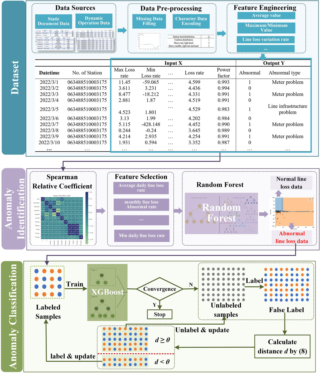
Figure 1. Framework of the proposed model.

3 Data pre-processing and feature engineering

In the process of abnormal line loss identification in a DN, the data pre-processing and feature engineering of substation operation data are essential. By processing and extracting features from substation operation data, accurate and comprehensive features can be obtained, effectively improving the accuracy and reliability of abnormal line loss identification in a DN.

Substation data in distribution networks can be divided into two categories. One is static document data, including DN topology data, customer relationship data, the number of users, load type, transformer type, and substation load distribution. The other is dynamic operation data, including the daily input and output electricity, daily line loss rate, daily power factor, daily maximum load rate, daily voltage compliance rate, and daily three-phase imbalance degree, which is shown in Table 1. For dynamic document data, not only data pre-processing, such as data cleaning and completion, need to be carried out but also relevant features need to be extracted. For example, statistical measures of line loss rate, such as the average value, maximum, minimum, and variance, are significantly related to the state of line loss. The overall data processing and feature engineering processes are shown in Figure 2.

Table 1

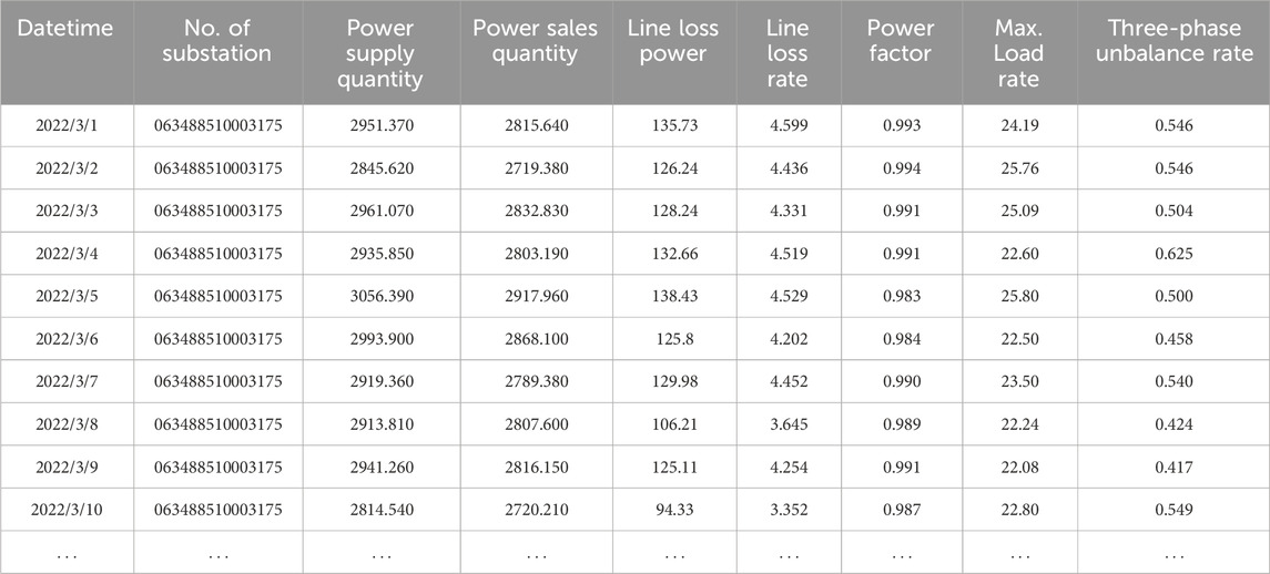
Table 1. Examples of dynamic operation data.

Figure 2

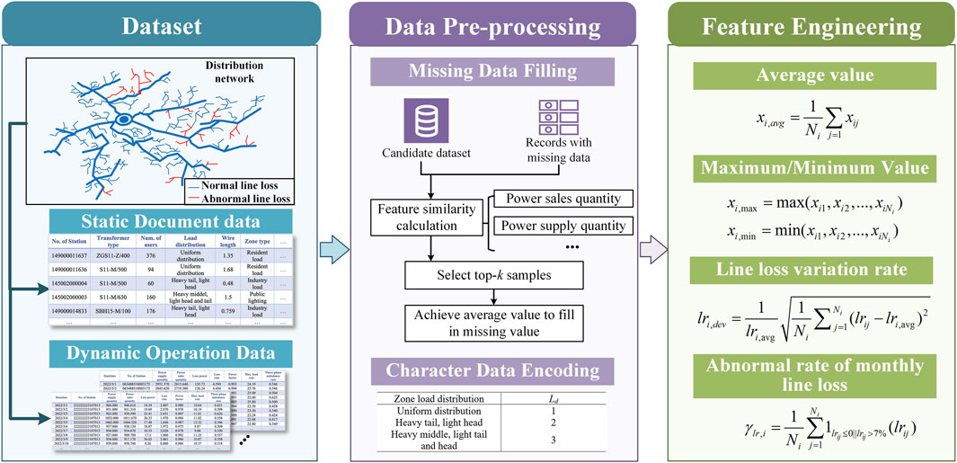
Figure 2. Data pre-processing and feature engineering.

3.1 Data pre-processing

Data pre-processing mainly includes filling in missing values and encoding character data.

(1) Character data encoding

Character data encoding is carried out for the load distribution L_d and abnormal line loss categories in the substation area. Table 2 shows character data encoding for the load distribution in the substation area.

(2) Missing data filling

Table 2

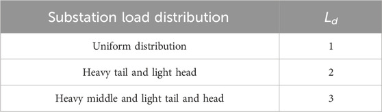
Table 2. Character data encoding of substation load distribution.

Upon the analysis of existing data, there were some missing data such as the daily power factor and daily three-phase unbalance in some substations. To solve this problem, the candidate set is generated by the substation. Then, the k-nearest neighbor method is adopted to select the k-samples which are the most similar from the candidate set and fill in the missing values by taking the average value of k-samples.

3.2 Feature engineering

According to the substation operation data, feature extraction is carried out on the daily power supply quantity, daily power sales quantity, daily line loss rate, daily power factor, and other data. The statistical features such as the average value, maximum value, minimum value, and variance in monthly are generated.

(1) Monthly average value

For the loss rate, lr; power factor, μ; maximum load rate, MaxL; and the three-phase voltage unbalance rate, U, the average value is calculated with the month as the statistical length, as shown in Equation 1:

$x_{i,\text{avg}}=\frac{1}{N_i}{\displaystyle \sum _{j=1}}{x}_{ij},(1)$

where x_ij indicates the measured value of the j-th day of the i-th month; x = lr, μ, MaxL or U; x_i,avg indicates the average value of the indicator in the i-th month; and N_i indicates the total number of days in the i-th month.

(2) Monthly maximum/minimum value

For the daily line loss rate lr and daily maximum load rate MaxL, the maximum and minimum values are calculated with the monthly statistical length, which is defined by Equation 2.

$\begin{array}{l}{x}_{i,\max }=\max \left(x_{i1},x_{i2},...,x_{i{N}_i}\right)\\ x_{i,\min }=\min \left(x_{i1},x_{i2},...,x_{i{N}_i}\right)\end{array},(2)$

where x_ij represents the measured value of the corresponding index on the j-th day of the i-th month.

(3) Monthly fluctuation rate of daily line loss

The fluctuation of the monthly line loss rate can also reflect the abnormality of the line loss to a certain extent. Considering the difference of the average line loss rate in months, the fluctuation rate of the monthly line loss is defined as in Equation 3 in order to remove the impact of the average level of the line loss rate on the statistical results.

$l{r}_{i,dev}=\frac{1}{l{r}_{i,\text{avg}}}\sqrt{\frac{1}{N_i}{\sum }_{j=1}^{N_i}{\left(l{r}_{ij}-l{r}_{i,\text{avg}}\right)}^2},(3)$

where lr_i,avg represents the average value of the line loss rate in the i-th month.

(4) Monthly abnormal rate of daily line loss

If the daily line loss rate is 0, negative, or too high, to some extent, it implies that the line loss rate may also be abnormal. Therefore, in order to reduce the influence of the accidental occurrence of the abnormal daily line loss rate, this paper defines the abnormal rate of monthly line loss, γ_lr,i, as shown in Equation 4. In this paper, the threshold of the excessive line loss rate is set as 7%.

${\gamma }_{lr,i}=\frac{1}{N_i}{\displaystyle \sum _{j=1}^{N_i}}{1}_{l{r}_{ij}\le 0‖l{r}_{ij}>7\%}\left(l{r}_{ij}\right).(4)$

4 Abnormal line loss recognition based on random forest

Random forest is an inheritance algorithm based on several decision tree classifiers. The bootstrap resampling technology is used to repeatedly randomly extract parts of the samples from the original training set to form a new training set to train multiple decision trees. The final abnormal line loss identification results are obtained by combining the results of multiple independent decision trees. Compared with the single decision tree, it has higher accuracy and stability, as shown in Figure 3.

Figure 3

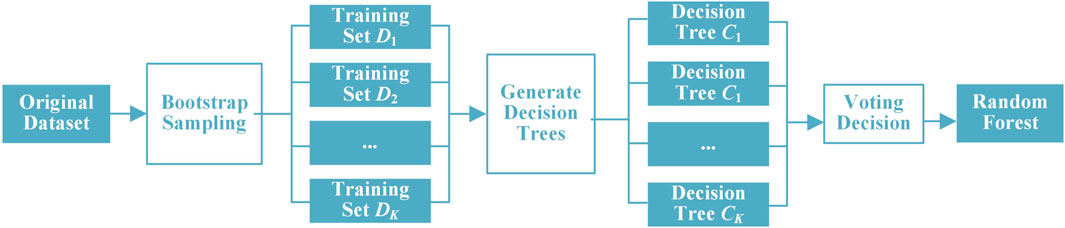
Figure 3. Illusion of random forest.

The features obtained by feature engineering are taken as the input of the random forest classifier, and the line loss abnormal is the output of the random forest classifier. Thus, the abnormal line loss identification of a DN is converted into a binary classification problem. The process is as follows:

Step 1. Dataset partitioning. The initial training set and the number of features are set. Based on the bootstrap resampling method, the samples from the original training set are repeatedly and randomly selected to form the training set D₁, … , D_K to build the single decision tree. The samples that have never been sampled are used to build validation datasets to estimate the performance of the model.

Step 2. Construction of a single decision tree. When constructing a single decision tree, each node is split through the principle of the minimum Gini index. When the Gini index is 0, all samples in the node belong to the same category. The Gini index is calculated as in Equation 5.

$Gini\left(D\right)=1-{{{\displaystyle \sum }}_{p=1}^P\left(\left|D_p\right|/\left|D\right|\right)}^2,(5)$

where |D| is the number of samples in the dataset, |D_p| is the number of samples belonging to class p in the set D, and P is the number of categories.

Step 3. Decision tree integration. In K decision trees, the Boyer–Moore majority vote algorithm is used to obtain the final classification result.

In the process of training the random forest, the depth of the decision tree M_t, the number of decision trees N_t, and the minimum number of samples in each split node S_t need to be determined. This paper uses grid search and cross-validation to determine the optimal hyperparameter combination.

5 Abnormal line loss category classification based on XGBoost and semi-supervised learning

To deal with the unlabeled sample problem, semi-supervised learning is employed. An initial model is first trained with labeled data and then used to predict the unlabeled samples. The labeled samples with high confidence are added to the labeled dataset and used to retrain the model to improve the classification accuracy.

5.1 XGBoost

XGBoost adopts the idea of boosting. The basic idea is to stack the base classifiers layer by layer. Each layer gives a higher weight to the misclassified samples of the previous layer when training. The XGBoost tree is constructed by extending a node into two branches, and the layers of the nodes continue to split until the entire tree is formed. Starting from the depth of the tree equal to 0, each node traverses all the features and sorts them according to the value of the feature gain function, as shown in Equation 6. In this way, all the features are sorted according to the contribution of the features to the objective function. Then, the feature is linearly scanned to determine the best segmentation point.

$Gain=\frac{1}{2}\left[\frac{G_L^2}{H_L+\lambda }+\frac{G_R^2}{H_R+\lambda }-\frac{{\left(G_R+G_L\right)}^2}{H_L+H_R+\lambda }\right]-\delta ,(6)$

where G_L represents the cumulative sum of the first-order partial derivation of the objective function by the samples contained in the left subtree after the current node splitting. G_R represents the cumulative sum of the first-order partial derivation of the objective function by the samples contained in the right subtree after the current node splitting. H_L represents the cumulative sum of the second-order partial derivation of the objective function by the samples contained in the left subtree after the current node splitting. H_R represents the cumulative sum of the second-order derivation of the objective function of the samples contained in the right subtree after the current node splitting. λ is the regularization parameter, and δ is the threshold to control the minimum gain of the split.

5.2 Abnormal line loss type classification based on XGBoost and semi-supervised learning

Since there are less labeled data for abnormal line loss types, most abnormal line losses only mark whether there is an anomaly but do not mark the specific reason of the anomaly. Therefore, this paper adopts the self-training semi-supervised learning method to model the abnormal line loss category classification. It trains an initial model with labeled data and then uses the model to predict the unlabeled data. The data with high confidence are added to the labeled dataset and used to retrain the model. The final model is obtained by iterating the process until the converge condition is satisfied.

According to whether the abnormal line loss type is labeled, the dataset is divided into the labeled sample dataset D_L = {(x₁, y₁), (x₂, y₂), …, (x_n, y_n)}and unlabeled sample dataset D_U. The number of sample label categories is N_c. In self-training semi-supervised learning, the pseudo-label sample selection strategy is the core part of the model performance. The purpose of the pseudo-labeled sample selection strategy is to select the samples that are more likely to be correctly labeled from the unlabeled samples and add them to the labeled samples to form a new training set so as to further improve the accuracy and generalization performance of the model. If pseudo-label samples, which are falsely labeled, are added to the training set, the performance of the model may be degraded. In this paper, pseudo-label sample selection based on the Mahalanobis distance is adopted, and the process is as follows:

In the labeled sample dataset D_L, the samples are divided according to the sample category. The sample set of class m is denoted as D_L,_m = {(x_i, y_i)| y_i = m}, m = 1, … , N_c. The average value of its feature vector is calculated based on Equation 7.

${\overline{\mathit{x}}}_m=\frac{1}{\left|{\mathbf{D}}_{\mathbf{L},m}\right|}{\displaystyle \sum _{\left({\mathit{x}}_i,y_i\right)\in {\mathbf{D}}_{\mathbf{L},m}}}{\mathit{x}}_i.(7)$

In the unlabeled sample dataset D_U, the corresponding pseudo-labeled sample set D_P is obtained after labeling. y_{p, j} is denoted as the pseudo-label of sample x_j, x_j ϵ D_U. Suppose y_{p, j} = m, the Mahalanobis distance between the pseudo-label sample (x_j, y_{p, j}) and ${\overline{\mathit{x}}}_m$ is calculated by Equation 8.

$d\left({\mathit{x}}_j,{\overline{\mathit{x}}}_m\right)=\sqrt{\left({\mathit{x}}_j-{\overline{\mathit{x}}}_m\right){\mathbf{C}}_m^{-1}{\left({\mathit{x}}_j-{\overline{\mathit{x}}}_m\right)}^{\mathrm{T}}},(8)$

where C_m is the covariance matrix of D_L,_m, which is shown in Equation 9.

${\mathbf{C}}_m=\frac{1}{\left|{\mathbf{D}}_{\mathbf{L},m}\right|-1}{\displaystyle \sum _{\left({\mathit{x}}_i,y_i\right)\in {\mathbf{D}}_{\mathbf{L},m}}}\left({\mathit{x}}_i-{\overline{\mathit{x}}}_m\right)\left({\displaystyle \sum _{\left({\mathit{x}}_i,y_i\right)\in {\mathbf{D}}_{\mathbf{L},m}}}{\mathit{x}}_i-{\overline{\mathit{x}}}_m\right).(9)$

The detailed processing of abnormal line loss category classification based on semi-supervised learning and XGBoost is shown as follows:

Step 1:. the XGB model, M, is built based on the dataset D_L = {(x₁, y₁), (x₂, y₂), …, (x_n, y_n)}.

Step 2:. the unlabeled sample set D_U is used as the input of model M. The corresponding pseudo-label is obtained to generate the pseudo-label sample set D_P.

Step 3:. the distance $d\left({\mathit{x}}_j,{\overline{\mathit{x}}}_m\right)$ based on Equation. 8 is calculated for each pseudo-label sample (x_j, y_{p, j}) ϵ D_p.

Step 4:. If $d\left({\mathit{x}}_j,{\overline{\mathit{x}}}_m\right)$ <θ, which is the threshold, it means that the pseudo-label is acceptable. The pseudo-label sample (x_j, y_{p, j}) is removed from D_P and added to D_L. If $d\left({\mathit{x}}_j,{\overline{\mathit{x}}}_m\right)$ ≥θ, it means that the pseudo-label is unreliable, and x_j is still retained in the unlabeled sample set D_U.

Step 5:. D_L and D_U are updated.

Step 6:. Steps 1–5 are repeated until the converge condition is satisfied. The final model is used to classify the category of abnormal line loss.

6 Experiment and results

6.1 Data source and experiment settings

In this paper, the operation data on three power supply stations in Lvliang, Shanxi Province, China, spanning half a year are used for comparison experiments. The three power stations contain 1,175 10-kV substations, which mainly include residential load, industrial load, public lighting, and commercial load. The substation operation data contain the daily active power supply, reactive power supply, line loss rate, input power, output power, power factor, maximum load rate, three-phase unbalance rate, and other data on substations spanning from May 2022 to November 2022.

In the experiment, the abnormality of the substation line loss is labeled by the month. There are a total of 7,050 samples in the dataset, including 1,503 abnormal line loss samples and 5,547 normal line loss samples. Due to the limited labor, only the abnormal causes in the part of the substation are verified, which includes 988 samples, accounting for 65.73% of the whole abnormal line loss samples. The distribution of abnormal line loss causes is shown in Figure 4. The main cause of abnormal line loss is the meter problem, including data acquisition exception and meter device fault. The electricity theft accounted for the smallest proportion. A part of the reason is that the electricity theft by users is difficult to confirm in reality due to user privacy. The detailed causes of different abnormal line loss categories are shown as follows:

• Line infrastructure problem: too long supply wire or too small wire radius and aging of the line equipment.

• Basic document files problem: distributed network topology mismatch and user-zone ownership error.

• Meter problem: data collected not at the same time, meter deviation, meter device failure, and communication failure.

• Theft of electricity: illegal use of electricity.

Figure 4

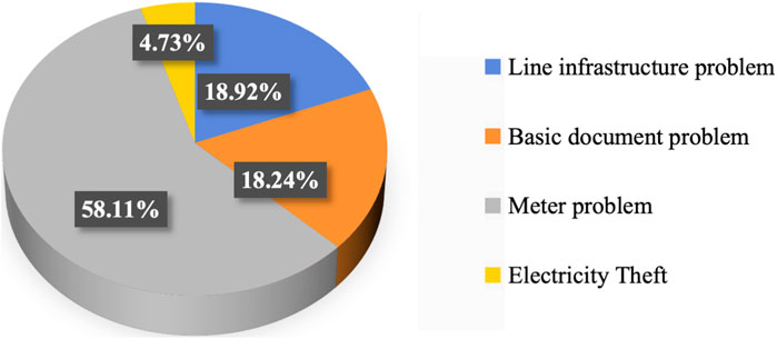
Figure 4. Diagram of abnormal line loss cause distribution.

In the abnormal line loss recognition model, the dataset is divided as 7:3, where 70% of the data comprises the training set and 30% of the data comprises the test set. The hyperparameters of the random forest and XGBoost model used in this paper are shown in Table 3.

Table 3

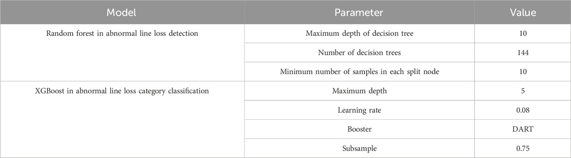
Table 3. Parameter settings.

In this paper, the abnormal line loss detection and category classification is a two-stage classification problem. Thus, the confuse matrix is used to display the result. In stage 1, the abnormal line loss identification is a binary classification problem.

In stage 2, the abnormal line loss category classification is a multi-classification task, and the evaluation metrics include accuracy, precision, recall, and the F1-score. Considering the unbalanced sample problem, this paper utilizes the macro average value, as shown in Equations 10–13. The TP is the number of the positive samples detected as positive. The TN is the number of negative samples detected as negative. The FP is the number of negative samples detected as positive. The FN is the number of positive samples detected as negative.

$Acc=\frac{1}{N_c}{\displaystyle \sum _{i=1}^{N_c}}\frac{T{P}_i+T{N}_i}{T{P}_i+F{P}_i+F{N}_i+T{N}_i},(10)$

$P=\frac{1}{N_c}{\displaystyle \sum _{i=1}^{N_c}}\frac{T{P}_i}{T{P}_i+F{P}_i},(11)$

$R=\frac{1}{N_c}{\displaystyle \sum _{i=1}^{N_c}}\frac{T{P}_i}{T{P}_i+F{N}_i},(12)$

$F_1=\frac{2\times P\times R}{P+R}.(13)$

6.2 Results of abnormal line loss identification and category classification

To further analyze the performance of feature engineering, the Spearman correlation analysis is first employed to quantify the relationship between the statistical features and abnormal line loss. The result is displayed in Figure 5. It is clear that the monthly abnormal rate of daily line loss, γ_lr,i, is the most important feature in abnormal line loss identification. The maximum value of line loss, the minimum value of line loss, and the average value of line loss also have a certain correlation with abnormal line loss. The three-phase unbalance rate is the least related to abnormal line loss and is not regarded as the input of the identification model.

Figure 5

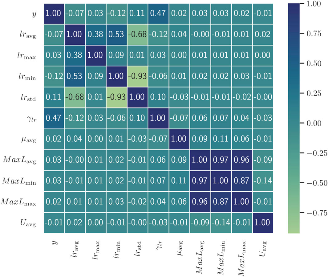
Figure 5. Correlation analysis of the statistical features.

The result of our proposed abnormal line loss identification and category classification model is shown in Table 4. It shows that a good performance is achieved in abnormal line loss identification. All the evaluation metrics obtain good results. Figure 6 displays the decision boundary of one decision tree of the random forest. It is clear that all the samples with negative line loss are recognized as abnormal. The sample with a high monthly abnormal rate and high minimal line loss rate is also identified as abnormal.

Table 4

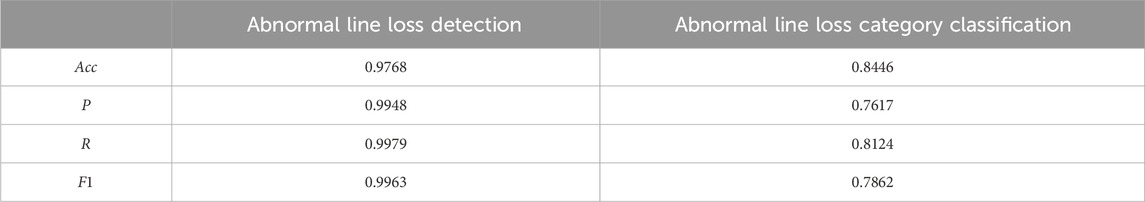
Table 4. Results of abnormal line loss detection and category classification.

Figure 6

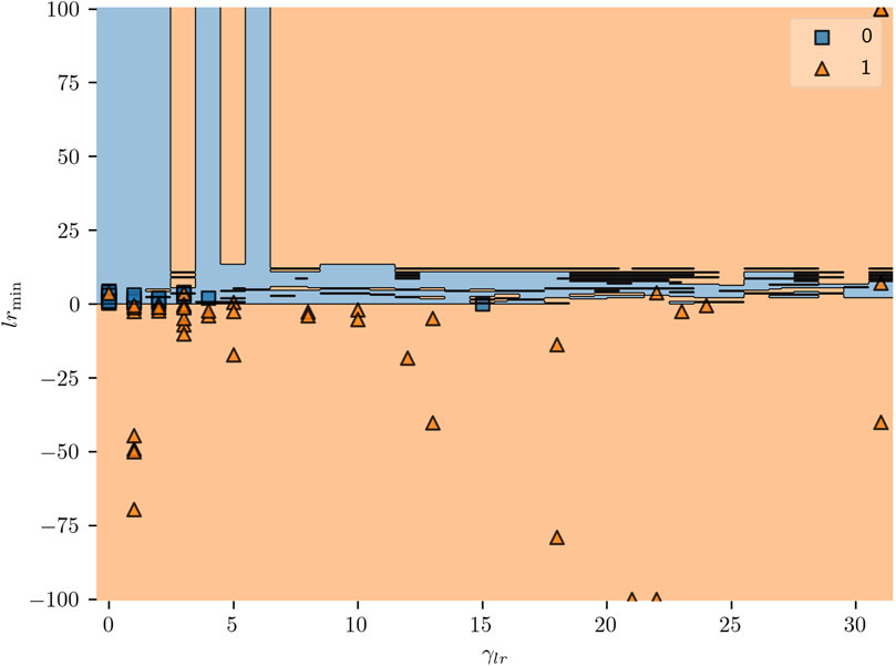
Figure 6. Diagram of the decision boundary of one decision tree of the random forest.

In abnormal line loss category, the classification result is not better than that of abnormal line loss identification. The small sample size and unbalanced sample distribution significantly impact the precision and recall values. The confusion matrix of the XGBoost model is presented in Figure 7. The classification result of electricity theft is the worst. The meter problem classification is the best. It is because the number of electricity theft incidents is too small and impacts the model learning. All the categories are easily misidentified as meter problems, especially electricity theft. In reality, the meter problem is the most common cause of abnormal line loss, including different abnormal line loss scenarios, such as data error, communication problem, and data collection terminal fault. Thus, other causes are easily misidentified as meter problems.

Figure 7

Figure 7. Confusion matrix of abnormal line loss category classification with XGBoost and semi-supervised learning. Label “Document” denotes the basic document files problem. Label “Theft” denotes theft of electricity. Label “Infrastructure” denotes the line infrastructure problem. Label “meter” denotes the meter problem.

6.3 Comparison experiment

In this section, the comparison experiments are conducted from different aspects, including abnormal line loss identification with different algorithms, abnormal line loss category classification with different algorithms, and comparison of supervised learning and semi-supervised learning.

1) Comparison of abnormal line loss identification with different algorithms

In abnormal line loss identification, the decision tree (DT), XGBoost, BP, and support vector machine (SVM) are utilized as the comparison algorithms. In DT, the max depth of tree is set as 12. In XGBoost, the learning rate is 0.1 and the number of estimators is set as 100. In BP, the number of hidden layers is set as 2, with 100 neurons in each hidden layer. The kernel function of SVM is the radial basis kernel function, and the regularization parameter is 1.

The identification results of different algorithms are shown in Figure 8. Since the abnormal line loss identification problem is a relatively simple binary classification problem, all the algorithms can achieve a good performance. From the aspect of accuracy, BP achieves the best performance. The accuracy values of RF, DT, XGBoost, and SVM are close. From the aspect of all metrics, the RF performs the best. The precision, recall, and F1-score of the RF are the highest. The precision result of BP implies that the model easily launches false alarms than RF. The performance of DT and SVM is the worst. Further analyzing the result with data, it is found that the monthly line loss with the negative daily line loss rate is easily recognized as abnormal. The abnormal monthly line loss with a small and positive line loss is the most difficult to detect compared to other abnormal line loss scenarios.

2) Comparison of abnormal line loss category classification with different algorithms

Figure 8

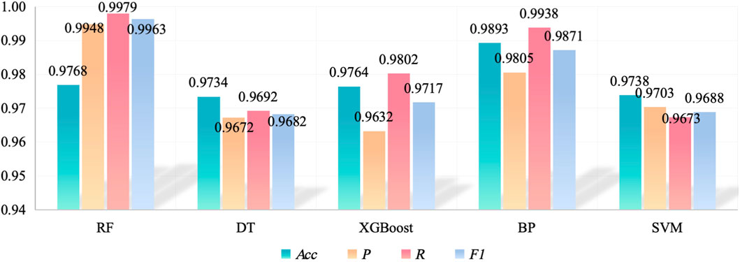
Figure 8. Results of abnormal line loss detection with different algorithms.

In abnormal line loss category classification, random forest, DT, and BP are used as the comparison algorithms. In random forest, the number of decision trees is set as 105, and the maximum depth of the decision tree is set as 10. In DT, the maximum depth of the tree is set as 15. In BP, the number of hidden layers is set as 3, with 85 neurons in each hidden layer. All the algorithms are conducted with the semi-supervised learning.

The result of the abnormal line loss category classification is displayed in Figure 9. It is obvious that the performance of XGBoost is the best and that of DT is the worst. Due to limited samples, the accuracy of abnormal line loss category classification is not higher than that of abnormal line loss identification. In another aspect, the input feature is generated based on monthly line loss, which cannot reflect the fluctuation of the intra-day line loss rate. In particular, the theft of electricity is closely related to the intra-day line loss rate, which cannot be well-detected.

3) Supervised learning vs. semi-supervised learning

Figure 9

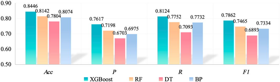
Figure 9. Results of abnormal line loss category classification with different algorithms.

In this section, the performance of supervised learning and semi-supervised learning is compared with XGBoost in the abnormal line loss category classification task. The supervised learning directly uses 70% of the labeled samples to train XGBoost, and the rest 30% was used for the test. The evaluation metric results are displayed in Table 5. From Table 5, it is obvious that the classification results are significantly improved by semi-supervised learning, especially recall. It is implied that the phenomenon of leaking alarm is relieved. The category of theft of electricity is the most difficult to detect. It is because of the limited electricity theft samples and because electricity theft is mostly impacted by the intra-day line loss rate. The confusion matrix of supervised learning is presented in Figure 10. Compared to Figure 7, the classification accuracy of all the categories is enhanced. For the semi-supervised learning, the unlabeled samples are used, which can help the model learn to increase the classification accuracy. However, the current data cannot reflect the situation of intra-day line loss, and the category classification performance is limited. To further improve the abnormal line category classification, detailed line loss data are needed.

Table 5

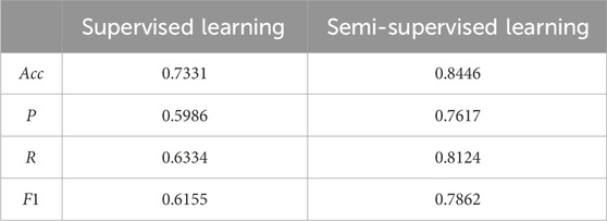
Table 5. Results of supervised learning and semis-supervised learning with XGBoost.

Figure 10

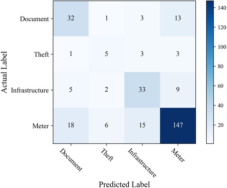
Figure 10. Confusion matrix of abnormal line loss category classification with XGBoost and supervised learning. Label “Document” denotes the basic document files problem. Label “Theft” denotes theft of electricity. Label “Infrastructure” denotes the line infrastructure problem. Label “meter” denotes the meter problem.

7 Conclusion

Abnormal line loss identification is crucial in distribution networks to guarantee the timely and safe power supply in grid. In actual situations, the cause of abnormal line loss is not completely labeled due to the expensive labor cost. Considering the actual limited and unbalanced samples, this paper proposed a hierarchical classification framework to identify the causal reason of the abnormal line loss. An abnormal line loss identification model-based random forest was first established to identify whether substation line loss was abnormal. Based on the results of detected abnormal line loss, an abnormal line loss category classification model was developed with semi-supervised learning and XGBoost, considering the unlabeled samples. With the help of self-training semi-supervised learning, the unlabeled samples were utilized to train the classification model to relieve the over-fitting performance. Numerous experiments were conducted on the real dataset from China. The accuracy of abnormal line loss identification was more than 97%. The accuracy of abnormal line loss category classification was around 84% under semi-supervised learning. The results highlight the good performance of the proposed hierarchical learning structure to relieve the impact of the unbalance samples, which is very helpful for future application.

In the future, more detailed abnormal line loss causes can be considered. In addition, the sampling techniques to relieve the sample unbalance can be further utilized when considering the detailed abnormal line loss causes. In summary, this research highlights the application of machine learning in abnormal line loss identification and category classification, with implications for improving the management and operation of power grids.

Data availability statement

The original contributions presented in the study are included in the article/supplementary material; further inquiries can be directed to the corresponding author.

Author contributions

WeL: writing–review and editing and writing–original draft; WeZ: writing–review and editing, writing–original draft, and data curation; JuL: writing–review and editing; JiL: writing–review and editing; YZ: writing–review and editing.

Funding

The author(s) declare financial support was received for the research, authorship, and/or publication of this article. This research was funded by the science and technology project of State Grid Shanxi Electric Power Company, grant number 5205J0220002. The funder was not involved in the study design, collection, analysis, interpretation of data, the writing of this article, or the decision to submit it for publication.

Conflict of interest

Authors WeL, WeZ, JuL, JiL, and YZ were employed by State Grid Shanxi Electric Power Company.

Publisher’s note

All claims expressed in this article are solely those of the authors and do not necessarily represent those of their affiliated organizations, or those of the publisher, the editors, and the reviewers. Any product that may be evaluated in this article, or claim that may be made by its manufacturer, is not guaranteed or endorsed by the publisher.

References

Buzau, M. M., Tejedor-Aguilera, J., Cruz-Romero, P., and Gómez-Expósito, A. (2020). Hybrid deep neural networks for detection of non-technical losses in electricity Smart meters. IEEE Trans. Power Syst. 35, 1254–1263. doi:10.1109/tpwrs.2019.2943115

CrossRef Full Text | Google Scholar

Chen, J., Zeb, A., Sun, Y., and Zhang, D. (2023b). A power line loss analysis method based on boost clustering. J. Supercomput. 79, 3210–3226. doi:10.1007/s11227-022-04777-w

CrossRef Full Text | Google Scholar

Chen, J. D., Nanehkaran, Y. A., Chen, W. R., Liu, Y. J., and Zhang, D. F. (2023a). Data-driven intelligent method for detection of electricity theft. Int. J. Electr. Power and Energy Syst. 148, 108948. doi:10.1016/j.ijepes.2023.108948

CrossRef Full Text | Google Scholar

Du, G., Zhang, J., Zhang, N., Wu, H., Wu, P., and Li, S. (2024). Semi-supervised imbalanced multi-label classification with label propagation. Pattern Recognit. 150, 110358. doi:10.1016/j.patcog.2024.110358

CrossRef Full Text | Google Scholar

Gunturi, S. K., and Sarkar, D. (2021). Ensemble machine learning models for the detection of energy theft. Electr. Power Syst. Res. 192, 106904. doi:10.1016/j.epsr.2020.106904

CrossRef Full Text | Google Scholar

Huang, L., Zhou, G., Zhang, J., Zeng, Y., and Li, L. (2023). Calculation method of theoretical line loss in low-voltage grids based on improved random forest algorithm. Energies 16, 2971. doi:10.3390/en16072971

CrossRef Full Text | Google Scholar

Jiang, W., and Tang, H. B. (2020). Distribution line parameter estimation considering dynamic operating states with a probabilistic graphical model. Int. J. Electr. Power and Energy Syst. 121, 106133. doi:10.1016/j.ijepes.2020.106133

CrossRef Full Text | Google Scholar

Jing, T. T., Dai, L., Xi, H. J., and Hu, Y., (2019). Method for theoretical line loss calculation of 10kV distribution district based on actual electric energy of distribution transformer secondary side. Iop Int. Conf. Civ. Archit. Disaster Prev. 218, 1–6. doi:10.1088/1755-1315/218/1/012152

CrossRef Full Text | Google Scholar

Liang, C., Chen, C., Wang, W., Ma, X., Li, Y., and Jiang, T. (2022). Line loss interval algorithm for distribution network with DG based on linear optimization under abnormal or missing measurement data. Energies 15, 4158. doi:10.3390/en15114158

CrossRef Full Text | Google Scholar

Lin, Y. Z., and Abur, A. (2018). A new framework for detection and identification of network parameter errors. IEEE Trans. Smart Grid 9, 1698–1706. doi:10.1109/tsg.2016.2597286

CrossRef Full Text | Google Scholar

Liu, K. Y., Jia, D. L., Kang, Z. J., and Luo, L. (2022). Anomaly detection method of distribution network line loss based on hybrid clustering and LSTM. J. Electr. Eng. Technol. 17, 1131–1141. doi:10.1007/s42835-021-00958-4

CrossRef Full Text | Google Scholar

Luo, F. Z., Yang, X., Yao, L. Z., Zhu, L. Z., Zhao, D. W., and Qian, M. H. (2021). “Flexible load active management method in optimization operation of distribution networks,” in Proceedings of the 2021 3rd asia energy and electrical engineering symposium (AEEES 2021), Chengdu, China 413–418. doi:10.1109/AEEES51875.2021.9403086

CrossRef Full Text | Google Scholar

Raghuvamsi, Y., Teeparthi, K., and Kosana, V. (2022). A novel deep learning architecture for distribution system topology identification with missing PMU measurements. Results Eng. 15, 100543. doi:10.1016/j.rineng.2022.100543

CrossRef Full Text | Google Scholar

Sayed, M. A., and Takeshita, T. (2011). All nodes voltage regulation and line loss minimization in loop distribution systems using UPFC. IEEE Trans. Power Electron. 26, 1694–1703. doi:10.1109/tpel.2010.2090048

CrossRef Full Text | Google Scholar

Sun, B., Li, Y. F., Zeng, Y., Chen, J. H., and Shi, J. D. (2022). Optimization planning method of distributed generation based on steady-state security region of distribution network. Energy Rep. 8, 4209–4222. doi:10.1016/j.egyr.2022.03.078

CrossRef Full Text | Google Scholar

Sun, Z., Xuan, Y., Huang, Y., Cao, Z., and Zhang, J. (2023). Traceability analysis for low-voltage distribution network abnormal line loss using a data-driven power flow model. Front. Energy Res. 11, 832837. doi:10.3389/fenrg.2023.1272095

CrossRef Full Text | Google Scholar

Van, E., Jesper, E., and Hoos, H. H. (2022). A survey on semi-supervised learning. Mach. Learn. 109 (2), 373–440. doi:10.1007/s10994-019-05855-6

CrossRef Full Text | Google Scholar

Wang, W., Bai, R., He, X., Xing, Y., Zhang, H., and Liu, J. (2019). “Development of synchronous line loss analysis and diagnosis system based on arbitrary segmentation of power grid,” in Proceedings of the 2019 IEEE 4th advanced information technology, electronic and automation control conference (IAEAC), Chengdu, China 1840–1844.

Google Scholar

Wu, W., Cheng, L., Zhou, Y., Xu, B., Zang, H., Xu, G., et al. (2019). Benchmarking daily line loss rates of low voltage transformer regions in power grid based on robust neural network. Appl. Sci. 9, 5565. doi:10.3390/app9245565

CrossRef Full Text | Google Scholar

Yao, M., Zhu, Y., Li, J., Wei, H., and He, P. (2019). Research on predicting line loss rate in low voltage distribution network based on gradient boosting decision tree. Energies 12, 2522. doi:10.3390/en12132522

CrossRef Full Text | Google Scholar

Zhang, Z. L., Yang, Y., Zhao, H., and Xiao, R. (2022). Prediction method of line loss rate in low-voltage distribution network based on multi-dimensional information matrix and dimensional attention mechanism-long-and short-term time-series network. Transm. Distribution 16, 4187–4203. doi:10.1049/gtd2.12590

CrossRef Full Text | Google Scholar

Zhou, S., Xue, J., Feng, Z., Dong, S., and Qu, J. (2022). “Abnormal line loss data detection and correction method,” in Proceedings of the 2022 4th asia energy and electrical engineering symposium (AEEES), Chengdu, China 832–837. doi:10.1109/AEEES54426.2022.9759815

CrossRef Full Text | Google Scholar

Zhu, L. P., and Lin, J. J. (2021). Learning spatiotemporal correlations for missing noisy PMU data correction in Smart grid. IEEE Internet Things J. 8, 7589–7599. doi:10.1109/jiot.2020.3040195

CrossRef Full Text | Google Scholar